 Open Access Article
 This Open Access Article is licensed under a
 Creative Commons Attribution 3.0 Unported Licence
Calculations of flow-induced orientation distributions for analysis of linear dichroism spectroscopy†
James R. A.
McLachlan
a,
David J.
Smith
b,
Nikola P.
Chmel
c and
Alison
Rodger
*c
aMolecular Organisation and Assembly in Cells Doctoral Training Centre, University of Warwick, Coventry CV4 7AL, UK
bSchool of Mathematics, University of Birmingham, Edgbaston, Birmingham B15 2TT, UK
cWarwick Centre for Analytical Science, Department of Chemistry, University of Warwick, Coventry CV4 7AL, UK. E-mail: A.Rodger@warwick.ac.uk
First published on 5th April 2013
Abstract
Spectroscopic techniques involving flow-oriented samples and polarised light, such as linear dichroism (LD), are becoming increasingly useful to probe biomacromolecular assemblies. However, the magnitude of the signal and in some cases the shape of the spectrum are dependent on the distribution of the orientations of the molecules in the sample. Despite great progress in the modelling of dilute and semi-dilute suspension mechanics, these theories have had remarkably little impact on the community practising LD. We perform calculations with a model combining Brownian effects and rotations in a steady shear flow of a dilute suspension of rigid, rodlike particles. We calculate the time-dependent probability density functions for the orientation distributions of three biomolecular assemblies: M13 bacteriophage, DNA molecules of well-defined length, and FtsZ protofilaments. Our calculations allow us to compute directly (rather than infer from experiment) the LD orientation parameter, S, for such assemblies. The results from the model are consistent with experiment for M13 bacteriophage and allow us to estimate S empirically for reasonably short DNA molecules. In analysing the particle size distribution for the process of FtsZ polymerisation, we find that results from the model aid our understanding of the process.
1 Introduction
Many interesting components of biological systems are large, comparatively irregular, assemblies of smaller components which are extremely hard to characterise structurally. Such systems include DNA polymers, fibrous proteins of the cytoskeleton, and lipid environments. In general, these systems are too large for study by nuclear magnetic resonance spectroscopy and too irregular for crystallography, and so one must resort to a library of complementary biophysical techniques. We have been developing linear dichroism (LD) spectroscopy,1–8 which requires the system of interest to be oriented during the experiment. Sufficient orientation is obtained to measure experimental signals for a wide range of systems when the samples are suspended in aqueous solution and subjected to shear flow with shear rates of the order of 1000 s−1. The magnitude of the reduced LD signal, LDr, for an ideal single molecule may be expressed as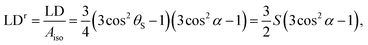 | (1) |
Our ability to use LD quantitatively to determine geometric information has been hindered by the fact that we often have little idea of the value of S. Sometimes an internal standard (e.g., the bases of DNA in a DNA–ligand complex9,10) provides this information. In other cases we have been limited to qualitative and comparative data analysis. However, the mechanics of dilute and semi-dilute suspensions is an intensively studied subject in mathematical fluid dynamics;11,12 it is therefore of great interest to apply these theories to flow linear dichroism of biological components, and to test the limits of their validity.
The study of the orientation of anisotropic particles in shear flow and their effect on fluid rheology began with the work of Jeffery,13 who, by neglecting Brownian motion and particle inertia, showed that isolated ellipsoids follow the flow velocity and perform a deterministic periodic rotation, now known as a Jeffery orbit. Eisenschitz14 applied Jeffery's theoretical analysis to model the orientation distribution of a suspension of such particles, based on the assumption of uniform initial orientation distribution. This assumption leads to time-periodic rheology, and as shown by Leal and Hinch,15,16 weak Brownian effects result in a singular perturbation problem: the distribution predicted by Eisenschitz's theory is not the limiting case as Brownian effects approach zero.
Peterlin and Stuart17 developed the theory of dilute suspensions of particles subject to shear flow and Brownian rotation, the orientation distribution evolving under the Fokker–Planck equation. Their solution was written as a triple sum expansion in spherical harmonics, now known as the Peterlin distribution, parameterised by the Péclet number (which quantifies the relative importance of shear forces and Brownian rotations) and particle slenderness ratio. While early studies were limited to determining coefficients for restricted cases, such as nearly spherical particles or weak Brownian effects, with the advent of digital computers it became possible to calculate more coefficients of the distribution numerically,18 and hence the ranges of particle slenderness and Péclet number over which valid results could be calculated were extended.
Later work involved rewriting the Peterlin distribution as a double sum19,20 and extending the parameter space investigated, although the focus remained on the steady-state distribution function rather than its dynamic onset. The hydrodynamic approach described in Strand et al.21 focused on the limiting case of infinitely slender particles, and extended the numerical approach to take account of temporal dynamics and a broader range of Péclet numbers. This last technique is the basis for our study.
Nordh et al. used a rotating rod model which neglected Brownian effects to fit an experiment conducted at a single, very low shear rate, and where both assembly and orientation dynamics would have been present.22 Investigation across a range of shear rates, with particles of well-controlled length and with Brownian rotations taken into account (as shown to be necessary by Leal and Hinch15), is therefore warranted.
The Peterlin distribution was used by Nordén et al. to calculate an orientation for DNA–RecA complexes which was consistent with small-angle neutron scattering patterns for 60 particles under shear flow.23 As a result, the authors adopted a value of S = 0.09 for shear rates above 200 s−1 even though the LD did not reach a limit in their experiments. The shape of the orientation distribution function and particle aspect ratio and Péclet number producing S = 0.09 were not reported.
Mikati et al.24 used earlier calculations of the steady-state Peterlin–Stuart coefficients20 to predict the value of the orientation function of both finitely and infinitely slender rods for various Péclet numbers (equivalent to the range 0–20 with our designation of Péclet number, and also the case of infinite Péclet number). A “fair” match between theory and experimental measurement of turbidity linear dichroism was reported, comparisons being made for specific fixed theoretical values of molecular length at different times in the dynamic assembly process. Additionally, predictions and experimental measurements of scattering and absorptive linear dichroism with microtubules were found to vary similarly as shear rate was varied. While this earlier work was restricted to the steady-state orientation of microtubules undergoing assembly and relatively low shear rates, in the present study we explore higher shear rates, considerably more elongated biological particles (including those of well-controlled length), and the temporal dynamics of orientation.
The aim of the present study is to determine to what extent we can use values of S calculated from a Brownian shear-orientation model of rigid fibres to interpret experimental data. The specific test applications considered in this work are to rigid, rodlike particles with the dimensions of M13 bacteriophage,25 linear DNA molecules,26 and FtsZ protofilaments.27
2 Methods
2.1 A Brownian shear-orientation model to calculate the orientation parameter
| sX = sin θsin ϕ, | (2a) |
| sY = cos θ, | (2b) |
| sZ = sin θcos ϕ, | (2c) |
| θS = arccos(|sin θcos ϕ|) | (3) |
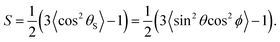 | (4) |
The shear flow velocity, u, is defined as (0, 0, kX), where k is the shear rate. Since uX = uY = 0, u = uZ = kX and the Y axis is the vorticity axis. The coordinate system is shown in Fig. 1.
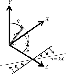 | ||
| Fig. 1 Coordinate system for an axisymmetric particle with orientation s in a shear flow. The Z axis is the laboratory-fixed spectroscopic orientation axis, and the Y axis is the vorticity axis. | ||
We now consider a dilute suspension of identical, rigid, neutrally buoyant, prolate-spheroidal particles. The suspended particles are sufficiently small that Brownian effects are significant; however, the size of the particles motivates us to take the local shear around each particle as uniform. Combining rotations in the shear flow and Brownian effects, and neglecting particle–particle interactions, we follow the formalism of Strand et al.21
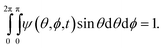
We introduce a probability density function, ψ, as the orientation distribution function for the suspended particles, where ψ(s)ds is the probability of finding a specific particle oriented in the solid angle ds about the orientation s. The normalisation condition for ψ as a function of time t is then
 | (5) |
For an initially isotropic distribution of particles, we require that ψ (θ, ϕ, 0) = 1/(4π). The change in particle orientation is given by
 | (6) |
The Péclet number determines the dynamics of the orientation distribution function. It is the dimensionless ratio of the convection time scale to the diffusion time scale. For Péclet number defined by Pλ = kλ, where λ is the material time constant,28 the governing Fokker–Planck equation for the orientation distribution may be written as
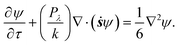 | (7) |
 | (8) |
 | (9) |
 | (10) |
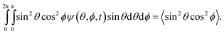
Solving eqn (7) reduces to solving a system of ordinary differential equations (ODEs) in time (Appendix B†). For each calculated Péclet number, we computed ψ(t) from the numerical solution to the ODEs. The orientation parameter, S(t), in eqn (4) followed from the numerical evaluation of
 | (11) |
2.2 Experimental data
We compared our own data and previously published data with results from the model described above. Our data were collected with either: (i) a Jasco J-815 circular dichroism spectropolarimeter adapted for LD measurements and a microvolume Couette cell described previously;7,30 or (ii) a new flow-through cell and a Biologic MOS-450 stopped-flow instrument.31 All data were obtained from experiments in the regime where signal is proportional to concentration.7DNA was purchased from Sigma-Aldrich (Gillingham, UK) and FtsZ was made as described by Pacheco-Gómez et al.32 Bacteriophage was kindly provided by T. R. Dafforn and M. R. Hicks (University of Birmingham, UK).
3 Results and discussion
The work summarised below was undertaken with the aim of understanding the behaviour in flow of three different biomolecular systems: M13 bacteriophage; linear DNA; and protofilaments of the bacterial cytoskeletal protein FtsZ (the protofilaments are polymers whose units are single FtsZ proteins). Values of S calculated from the model depend on both the length and width of the rods being considered. M13 bacteriophage are approximately 800 nm in length (all phage in a sample are the same) and 8 nm in diameter. They are very rigid, having a persistence length in excess of 1000 nm.25 B-DNA is approximately 2.37 nm wide and there are 0.34 nm steps between base pairs. Different DNA molecules have different numbers of bases in the polymer. Strictly, DNA is a semi-rigid rod, its persistence length being approximately 50 nm.33 (We return to this issue in Section 3.3.) FtsZ monomers, within protofilaments, are approximately 4.2 nm in length and 5.7 nm wide. Within any sample there is a distribution of polymer lengths. The best estimate of FtsZ protofilament persistence length is 1.15 ± 0.25 μm.34 In what follows we use the model to calculate S(t) from the onset of flow (M13 and derived particles), with shear rate as a parameter (M13 and DNA), and with particle length as a parameter (DNA and FtsZ).3.1 Orientation parameter as a function of time
We wanted to determine from the model how quickly and to what extent rods of different dimensions orient in shear flow. We calculated how quickly dilute solutions of rigid fibres in laminar flow achieve peak (steady-state) orientation. Fig. 2 shows the results for M13 phage (for which a = 400 nm, b = 4 nm, and r = 100) with shear rates in the range 20–2000 s−1 and for related particles of the same width but length 400 nm or 80 nm at a single shear rate (all plotted against dimensionless time τ for comparison). In summary, the shorter particles orient more quickly (owing to their smaller time scale λ) but to significantly less extent. Higher shear rates induce peak orientation more quickly. The calculations indicate that even for slow flow rates, particles can be deemed to reach peak orientation within 15 ms.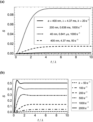 | ||
| Fig. 2 Orientation parameter, S, calculated from the model as a function of time for different particle sizes and shear rates at 22 °C. (a) Shorter particles (b = 4 nm in all cases) or lower shear rates. (b) Higher shear rates for M13 bacteriophage particles (λ = 4.37 ms). For sufficiently large Péclet numbers, the results give the well-known prediction for rigid rods of an overshoot followed by an undershoot.21 | ||
To test the relevance of the results summarised in Fig. 2 for our LD experiments, we measured orientation from the onset of shear flow in two types of flow cell: (i) an outer-rotating cylindrical microvolume Couette flow cell (3 mm internal diameter capillary with 2.5 mm stationary rod), giving homogeneous shear flow;7,35 and (ii) a square cross-section (1 mm × 1 mm) flow channel giving mean shear rate 124 s−1 (Appendix C†). In the former flow cell, we used M13 bacteriophage and 850 base pair poly(dA)–poly(dT) DNA (176 μM in base, a(contour) ≈ 150 nm, b = 1.2 nm, r ≈ 125). The shear rates were in the range 250–3000 s−1 (all laminar flow). The time to reach peak orientation at room temperature ranged from 40 ± 10 ms to 130 ± 30 ms (mean ± standard error of the mean from 10 measurements), with higher shear rates resulting in longer equilibration times. The fact that higher shear rates result in longer times to reach peak orientation implies that the duration of the orientation process is dominated by the initiation of the drive mechanisms that create the shear flow.
We conclude from these experiments and the results from the model that with the current sophistication of our instrumentation, the motor takes much longer to get to speed than the molecules do to reach peak orientation.
3.2 Steady-state orientation parameter as a function of shear rate
Given that the time dependence of the molecular orientation does not affect our experiments, we wanted to determine to what extent we could use steady-state values of S calculated from the model to interpret experimental data. The steady-state orientation parameter, S∞, calculated for M13 bacteriophage (Fig. 3) increases with shear rate, but remains below 0.6 (S = 1 for perfect orientation) at 22 °C. There is very little orientation (S∞ < 0.0075) for shear rates below 50 s−1, and then the increase is roughly linear with shear rate until 500 s−1, after which the rate of increase decreases.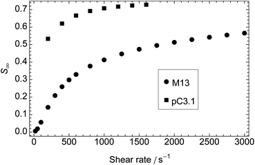 | ||
| Fig. 3 Steady-state orientation parameter, S∞, calculated from the model as a function of shear rate for M13 bacteriophage (a = 400 nm, b = 4 nm, r = 100) and plasmid DNA pC3.1 (6882 base pairs in length, a = 1170 nm, b = 1.2 nm, r = 975). Temperature: 22 °C for phage, 37 °C for DNA. | ||
The corresponding experimental data are shown in Fig. 4. Combining the experimental LDr206nm at 2000 s−1 (0.98) with the corresponding calculated S∞ (0.46) leads us to predict from eqn (1) that the transition contributing to the intensity at 206 nm is oriented at 26° ± 4° from the long axis of the phage. The 206 nm region of the spectrum is largely due to transitions polarised along the long axis of α-helices.36 Our prediction therefore accords well with the average helix orientation determined in Appendix D† to be ∼31°. This consistency supports the conclusion that for bodies as rigid as M13 bacteriophage we can use values of S∞ calculated from the model. To improve these estimates we need better absorbance data and to deconvolve the LD spectrum into component bands.37
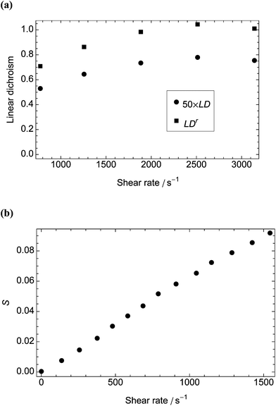 | ||
| Fig. 4 Measurements against shear rate for LD data collected in a microvolume Couette flow cell with outer and inner radii 3 mm and 2.75 mm, respectively. (a) LD206nm and LDr for M13 bacteriophage (0.01 mg mL−1). We used the absorbance of a 0.1 mg mL−1 protein solution (determined from Kelly et al.38 to be ∼0.015 at 206 nm) to calculate LDr. (b) Orientation parameter, S, of DNA plasmid pC3.1 (100 μM) at 37 °C with absorbance determined from assuming an average base extinction coefficient at 260 nm of 6600 mol−1 cm−1 dm3 (data derived from Rittman et al.33). | ||
The calculated dependence of S∞ on shear rate at 37 °C for a rigid, rodlike particle with the dimensions of a DNA plasmid variant of pC3.1 (6882 base pairs in length, a = 1170 nm, b = 1.2 nm, r = 975)33 is also shown in Fig. 3. This particle is longer and thinner than M13 and reaches higher orientations at lower shear rates with a higher peak value of S∞ (0.73), despite the higher temperature. The corresponding experimental plot (Fig. 4b), however, bears little relation to the plot from the model, the orientation parameter not reaching its limiting value before the loss of laminar flow in the cell. We address this discrepancy below.
3.3 Steady-state orientation parameter as a function of particle dimensions
Many samples studied by LD spectroscopy are not monodispersed; rather, they have a distribution of particle lengths. For some applications, such as probing ligand binding to DNA, an average value of S may be sufficient. However, to use LD to analyse the progress of a polymerisation reaction (e.g., the formation of FtsZ protofilaments), a more detailed understanding of the dependence of net signal on particle size distribution is required. Fig. 5 shows how the calculated S∞ of model particles with the dimensions of B-DNA and FtsZ protofilaments depends on particle length at fixed shear rates of 3000 s−1 and 1000 s−1, respectively.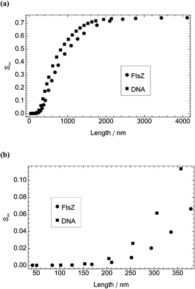 | ||
| Fig. 5 Steady-state orientation parameter, S∞, calculated from the model as a function of particle length for DNA molecules (width 2.37 nm and length in multiples of 0.34 nm) and FtsZ protofilaments (width 5.7 nm and length in multiples of 4.2 nm). Shear rate and temperature: 3000 s−1 and 37 °C for DNA; 1000 s−1 and 22 °C for FtsZ. (a) Particle length 42–4116 nm. (b) Particle length 42–378 nm. | ||
Experimental data for DNA molecules of different lengths (Fig. 6) are consistent with the calculations from the model for DNA molecules up to approximately 150 nm in length (i.e., ∼450 base pairs or three persistence lengths), where S < 0.01. For the longer DNA molecules, the experimental results are asymptotic to a maximal S which is an order of magnitude smaller than that calculated from the model. This observation is consistent with atomic force microscopy images39 which show DNA as bending back on itself and make clear that only short DNA molecules can be considered as rigid rods. For molecules longer than 750 nm (the usual DNA size for LD spectroscopy), the experimental value of S is ∼1/4 that calculated from the model for DNA of 1/12 the length; i.e., for experiments with a known length of DNA, one can use a value of S that is 25% of that calculated from the model for DNA of 8% the length (model at 37 °C and experiment at 22 °C).
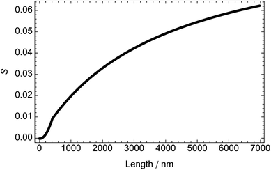 | ||
| Fig. 6 Dependence of orientation parameter, S, on DNA length at shear rate 3000 s−1 and temperature 22 °C (determined from experimental data in Rittman et al.33 and Simonson and Kubista40), assuming that α = 86° and the average base extinction coefficient is 6600 mol−1 dm3 cm−1. | ||
If we assume that FtsZ is sufficiently rigid for the model to be appropriate, we can use the calculated dependence of S on length from the model to understand what is happening in polymerisation experiments. FtsZ is typical of many fibrous proteins in that it is formed dynamically from monomers upon the addition of guanosine triphosphate (GTP). In our typical experiment,32,35,41 we mix Escherichia coli FtsZ (11 μM, molecular weight 40.3 kDa) with 0.2 mM GTP and observe the increase in LD at 210 nm while imposing a shear rate of 1000 s−1 in a microvolume Couette cell at room temperature. Most of the polymerisation occurs in the dead time of assembling the cell (40 s), the FtsZ having a steady-state LD210nm of 0.02 until the GTP is exhausted, after which it depolymerises.
In an alternate experiment, we used the aforementioned 1 mm × 1 mm flow cell (with the same concentrations of sample) to access the first three seconds of the reaction, after which an apparent steady-state LD of 0.001 is adopted when the shear rate is 248 s−1. This factor of 40 difference (path length is double) in S for the two systems is reproducible. From Fig. 3 we estimate that the S∞ values measured for the 1 mm × 1 mm cell are ∼1/4 those for the Couette cell. Thus we conclude that, between 3 s and 40 s in the polymerisation process, the average particle length must be increasing because of annealing of shorter particles. This is in accord with the assumptions of some of the models of FtsZ polymerisation; however, it has been assumed that the rate of annealing of long particles is equal to that of adding a monomer to a polymer.42 This is unlikely to be the case, but no method to measure the rate of annealing has previously been available. Below we outline how a combination of calculated dependence of S on particle length from the model and dynamic experimental LD data could be used to make better estimates of the annealing rate to aid modelling of such complex polymerisation processes.
Consider first the data from the steady-state LD signal at 40 s. The reduced LD (eqn (1)) can be determined if we have a value for the absorbance at 210 nm. The work of Kelly et al.38 tells us that a 1 mg mL−1 protein has an absorbance of ∼21 at 210 nm in a 1 cm path length cell, which makes the 210 nm absorbance of 11 μM FtsZ in a 0.5 mm path length Couette cell ∼0.47. Thus LDr210nm ≈ 0.02/0.47 ≈ 0.043. As outlined in Appendix D,† the average α-helix direction in FtsZ (which is the same as the 210 nm transition polarisation in proteins) is ∼48°. (Here, the average has been determined from the 〈cos2α〉 term in averaging LD.) Substituting these values into eqn (1) gives S ≈ 0.083 for the Couette cell experiment.
A combination of particle size distribution and the calculation from the model of S as a function of particle length enables an average S to be determined for a solution of FtsZ fibres. The FtsZ polymerisation reaction is formally equivalent to Flory's linear condensation reaction of polymers43 if, since GTP is in significant excess, we assume that FtsZ polymers are formed from reactions of monomer with monomer, monomer with polymer, and polymer with polymer. Replotting and fitting to the data in Fig. 3 and 4 of Flory's paper indicate that the fraction of polymers of a given length decreases exponentially with length (which is consistent with the distribution of the longer fibres that are visible in electron micrographs of FtsZ protofilaments32,34). According to Flory's model, the exponential function fitting our experimental values of S at 3 s and 40 s corresponds to a reaction that is 97% complete at 3 s and 99% complete at 40 s. To obtain the experimental value of S at 40 s, it follows that the protofilament size contributing the most monomers is ∼20 monomers in length. For the data at 3 s, this size is ∼16 monomers. Data for more time points would help our understanding of the dynamics of the particle size distribution.
At both time points there are small numbers of large particles, which contribute significantly per particle to the LD. These in vitro data support the view that the Z-ring in E. coli (500 nm in diameter) is not made of single protofilaments.42
3.4 Distribution of orientation angles of particles
From the model, we calculated the proportions of M13 bacteriophage particles that align with θS < 10°, 20° and 30° at shear rates 50–2000 s−1 and temperature 22 °C (Appendix E†). The results are plotted against time in Fig. S1† and compared with those in Fig. 2.We found that, for higher S (∼0.3–0.5), the proportion of particles with θS < 30° is close to the orientation parameter value. An orientation parameter of ∼0.5 implies that approximately one third of the particles in the sample will be oriented within 20° of the laboratory-fixed orientation axis. We also found that the proportion of particles with θS < 10° remains small (<0.1), even at the higher shear rates. Finally, between shear rates 50 s−1 and 200 s−1, there is a 44% increase in the steady-state proportion of particles with θS < 30°, but an eightfold increase in S∞.
4 Conclusion
In this work, we showed how to apply a model of dilute suspensions of rigid, rodlike particles in a steady shear flow with Brownian effects to the analysis of Couette-flow and flow-through linear dichroism spectroscopy. We tested the technique for M13 bacteriophage particles, FtsZ protofilaments, and DNA molecules. Our calculations allowed us to compute directly the orientation parameter for LD spectroscopy, a quantity one had previously to infer from experiment. Experimental data support the model and indicate how it may be used to aid our analysis of LD experiments and hence our understanding of biomolecular structure, processes and interactions.The model to calculate orientation distributions could be applied to other spectroscopic techniques, such as Raman linear difference spectroscopy,44 where the sample must be oriented during experiments.
Acknowledgements
We thank the Engineering and Physical Sciences Research Council for funding for a studentship for J. McL. (grant number EP/F500378/1) and the Biotechnology and Biological Sciences Research Council for equipment (grant number BB/F011199/1). D. J. S. was funded by a Birmingham Science City Research Alliance Fellowship. We are grateful to T. R. Dafforn and M. R. Hicks (University of Birmingham, UK) for providing bacteriophage.References
- B. M. Bulheller, A. Rodger, M. R. Hicks, T. R. Dafforn, L. C. Serpell, K. E. Marshall, E. H. C. Bromley, P. J. S. King, K. J. Channon, D. N. Woolfson and J. D. Hirst, J. Am. Chem. Soc., 2009, 131, 13305–13314 CrossRef CAS.
- T. R. Dafforn, J. Rajendra, D. J. Halsall, L. C. Serpell and A. Rodger, Biophys. J., 2004, 86, 404–410 CrossRef CAS.
- A. Damianoglou, A. Rodger, C. Pridmore, T. R. Dafforn, J. A. Mosely, J. M. Sanderson and M. R. Hicks, Protein Pept. Lett., 2010, 17, 1351–1362 CrossRef CAS.
- M. J. Hannon, V. Moreno, M. J. Prieto, E. Moldrheim, E. Sletten, I. Meistermann, C. J. Isaac, K. J. Sanders and A. Rodger, Angew. Chem., Int. Ed., 2001, 40, 880–884 CAS.
- M. R. Hicks, J. Kowałski and A. Rodger, Chem. Soc. Rev., 2010, 39, 3380–3393 RSC.
- M. R. Hicks, A. Rodger, C. M. Thomas, S. M. Batt and T. R. Dafforn, Biochemistry, 2006, 45, 8912–8917 CrossRef CAS.
- R. Marrington, T. R. Dafforn, D. J. Halsall, J. I. MacDonald, M. R. Hicks and A. Rodger, Analyst, 2005, 130, 1608–1616 RSC.
- B. Nordén, A. Rodger and T. R. Dafforn, Linear Dichroism and Circular Dichroism, Royal Society of Chemistry, Cambridge, UK, 2010 Search PubMed.
- K. K. Patel, E. A. Plummer, M. Darwish, A. Rodger and M. J. Hannon, J. Inorg. Biochem., 2002, 91, 220–229 CrossRef CAS.
- A. Rodger, I. S. Blagbrough, G. Adlam and M. L. Carpenter, Biopolymers, 1994, 34, 1583–1593 CrossRef CAS.
- S. Kim and S. J. Karrila, Microhydrodynamics: Principles and Selected Applications, Butterworth-Heinemann, Boston, MA, 1991 Search PubMed.
- E. Guazzelli and E. J. Hinch, Annu. Rev. Fluid Mech., 2011, 43, 97–116 CrossRef.
- G. B. Jeffery, Proc. R. Soc. London, Ser. A, 1922, 102, 161–179 CrossRef.
- R. Eisenschitz, Z. Phys. Chem., Abt. A, 1932, 158, 85 Search PubMed.
- L. G. Leal and E. J. Hinch, J. Fluid Mech., 1971, 46, 685–703 CrossRef.
- E. J. Hinch and L. G. Leal, J. Fluid Mech., 1972, 52, 683–712 CrossRef.
- A. Peterlin and H. A. Stuart, Z. Phys., 1939, 112, 129–147 CrossRef CAS.
- H. A. Scheraga, J. T. Edsall and J. O. Gadd, J. Chem. Phys., 1951, 19, 1101–1108 CrossRef CAS.
- W. E. Stewart and J. P. Sørensen, Trans. Soc. Rheol., 1972, 16, 1–13 CrossRef CAS.
- M. Nakagaki and W. Heller, J. Chem. Phys., 1975, 62, 333 CrossRef CAS.
- S. R. Strand, S. Kim and S. J. Karrila, J. Non-Newtonian Fluid Mech., 1987, 24, 311–329 CrossRef CAS.
- J. Nordh, J. Deinum and B. Nordén, Eur. Biophys. J., 1986, 14, 113–122 CrossRef CAS.
- B. Nordén, C. Elvingson, T. Eriksson, M. Kubista, B. Sjöberg, M. Takahashi and K. Mortensen, J. Mol. Biol., 1990, 216, 223–228 CrossRef.
- N. Mikati, J. Nordh and B. Nordén, J. Phys. Chem., 1987, 91, 6048–6055 CrossRef CAS.
- A. S. Khalil, J. M. Ferrer, R. R. Brau, S. T. Kottmann, C. J. Noren, M. J. Lang and A. M. Belcher, Proc. Natl. Acad. Sci. U. S. A., 2007, 104, 4892–4897 CrossRef CAS.
- B. Nordén, M. Kubista and T. Kurucsev, Q. Rev. Biophys., 1992, 25, 51–170 CrossRef.
- J. Löwe and L. A. Amos, Nature, 1998, 391, 203–206 CrossRef.
- R. B. Bird, O. Hassager, R. C. Armstrong and C. F. Curtiss, Dynamics of Polymeric Liquids: Vol. 2, John Wiley and Sons, New York, NY, 1977 Search PubMed.
- V. A. Bloomfield, Survey of Biomolecular Hydrodynamics, in Separations and Hydrodynamics, Biophysical Society, Bethesda, MD, 2000 Search PubMed.
- R. Marrington, T. R. Dafforn, D. J. Halsall and A. Rodger, Biophys. J., 2004, 87, 2002–2012 CrossRef CAS.
- X. Cheng, M. B. Joseph, J. A. Covington, T. R. Dafforn, M. R. Hicks and A. Rodger, Anal. Methods, 2012, 4, 3169–3173 RSC.
- R. Pacheco-Gómez, D. I. Roper, T. R. Dafforn and A. Rodger, PLoS One, 2011, 6, e19369 Search PubMed.
- M. Rittman, E. Gilroy, H. Koohy, A. Rodger and A. Richards, Sci. Prog., 2009, 92, 163–204 CrossRef CAS.
- D. J. Turner, I. Portman, T. R. Dafforn, A. Rodger, D. I. Roper, C. J. Smith and M. S. Turner, Biophys. J., 2012, 102, 731–738 CrossRef CAS.
- R. Marrington, E. Small, A. Rodger, T. R. Dafforn and S. G. Addinall, J. Biol. Chem., 2004, 279, 48821–48829 CrossRef CAS.
- N. A. Besley and J. D. Hirst, J. Am. Chem. Soc., 1999, 121, 9636–9644 CrossRef CAS.
- M. Rittman, S. V. Hoffmann, E. Gilroy, M. R. Hicks, B. Finkenstadt and A. Rodger, Phys. Chem. Chem. Phys., 2012, 14, 353–366 RSC.
- S. M. Kelly, T. J. Jess and N. C. Price, Biochim. Biophys. Acta, Proteins Proteomics, 2005, 1751, 119–139 CrossRef CAS.
- I. Meistermann, V. Moreno, M. J. Prieto, E. Moldrheim, E. Sletten, S. Khalid, P. M. Rodger, J. C. Peberdy, C. J. Isaac, A. Rodger and M. J. Hannon, Proc. Natl. Acad. Sci. U. S. A., 2002, 99, 5069–5074 CrossRef CAS.
- T. Simonson and M. Kubista, Biopolymers, 1993, 33, 1225–1235 CrossRef CAS.
- E. Small, R. Marrington, A. Rodger, D. J. Scott, K. Sloan, D. Roper, T. R. Dafforn and S. G. Addinall, J. Mol. Biol., 2007, 369, 210–221 CrossRef CAS.
- I. V. Surovtsev, J. J. Morgan and P. A. Lindahl, PLoS Comput. Biol., 2008, 4, e1000102 Search PubMed.
- P. J. Flory, J. Am. Chem. Soc., 1936, 58, 1877–1885 CrossRef CAS.
- P. Kowalska, J. R. Cheeseman, K. Razmkhah, B. Green, L. A. Nafie and A. Rodger, Anal. Chem., 2012, 84, 1394–1401 CrossRef CAS.
Footnote |
| † Electronic supplementary information (ESI) available. See DOI: 10.1039/c3sm27419e |
| This journal is © The Royal Society of Chemistry 2013 |