Modeling the response of dual cross-linked nanoparticle networks to mechanical deformation
Balaji V. S.
Iyer
a,
Isaac G.
Salib
a,
Victor V.
Yashin
a,
Tomasz
Kowalewski
b,
Krzysztof
Matyjaszewski
b and
Anna C.
Balazs
*a
aChemical Engineering Department, University of Pittsburgh, Pennsylvania 15261, USA. E-mail: balazs@pitt.edu
bDepartment of Chemistry, Carnegie Mellon University, Pennsylvania 15213, USA
First published on 29th October 2012
Abstract
We develop a hybrid computational model for the behavior of a network of cross-linked polymer-grafted nanoparticles (PGNs). The individual nanoparticles are composed of a rigid core and a corona of grafted polymers that encompass reactive end groups. With the overlap of the coronas on adjacent particles, the reactive end groups can form permanent or labile bonds, which lead to the formation of a “dual cross-linked” network. To capture these multi-scale interactions, our approach integrates the essential structural features of the polymer grafted nanoparticles, the interactions between the overlapping coronas, and the kinetics of bond formation and rupture between the reactive groups on the chain ends. Via this model, we determine the tensile properties of the dual cross-linked samples. We find that the mechanical behavior of the network can be tailored by altering the bond energies of the labile bonds, the fraction of permanent bonds in the network and the thickness of the polymer corona. In particular, for a network with weaker labile bonds, an increase in fraction of permanent bonds and the contour length of the chain can yield a tough network that behaves like a polymeric material, which exhibits cold drawing/necking. On the other hand, similar changes to the network with stronger labile bonds lead to an increase in toughness, with the network characteristics being similar to that of a purely ductile material. Variations in the ratio between the strain rate and the bond rupture rate are also found to affect the response of the networks. Our model provides a powerful approach for predicting how critical features of the system affect the performance of cross-linked polymer-grafted nanoparticles.
I. Introduction
Advances in the grafting of polymer chains onto nanoparticles now permit significant control over the type and number of chains that can be anchored.1–5 Through the appropriate functionalization of these grafted chains, the coated nanoparticles can be interconnected into extensive networks. Recent studies have revealed that these nanoparticle networks can exhibit remarkable mechanical properties.6–10 There are, however, few theoretical or computational models,11–13 that can provide useful guidelines for tailoring the properties of the functionalized chains to yield the desired mechanical properties in networks of polymer grafted nanoparticles (or “PGNs”). The problem becomes particularly challenging and intriguing in light of recent developments on the utility of harnessing “dual cross-links” to optimize the mechanical properties of networks.14–20 Dual cross-linked systems are inter-connected by both strong and weak bonds. Recent computational studies involving nanoscopic gel particles (“nanogels”)15,16 showed that the dual cross-linked nanogels could exhibit greater strength and ductility than the materials that were cross-linked solely by the strong, permanent bonds. This dual cross-linking strategy could be applied not only to soft nanogels, but also hard, functionalized nanoparticles and thus, can potentially lead to novel materials with beneficial mechanical properties.There are, however, a number of issues that must be addressed in designing such advantageous PGN networks. While the soft nanogels provide a useful degree of elasticity, the polymers grafted onto the rigid nanoparticles must now impart the desired flexibility. Furthermore, the grafted polymers must be functionalized with the appropriate reactive groups in order to achieve an effective dual cross-linking. These constraints introduce a number of design variables, such as the length of the grafted chains and the interaction energies between reactive groups; these factors will play an important role in dictating the overall mechanical behavior of the composite.
The appropriate computational models would greatly facilitate the design of such hybrids materials. Such computational studies are challenging because all the relevant length and time scales should be captured in one specific model. Namely, the model must span a range of architectural features and temporal events. Herein, we develop an approach that encompasses the following components: (1) the essential structural features of the polymer grafted nanoparticles, (2) the interactions between the coated particles, (3) the kinetics of bond formation and rupture between the reactive groups on the coating, and (4) the resulting global response of a macroscopic sample to an applied force, which we take to be a tensile deformation. Our new approach extends the capabilities of prior models15,16 by now describing effects resulting from physical and chemical interactions between polymeric coronas that surround rigid nanoparticles. Specifically, the previous models15,16 did not explicitly include the presence of long, grafted chains, and thus, could not account for effects that arise from varying the length or density of polymers grafted onto the nanoscopic cores. Hence, with this new model, we can establish guidelines for tailoring the strength and toughness of nanoparticles with grafted polymers.10
Using this multi-component model, we can determine how such parameters as the fraction of labile bonds in the network, the bond energies of the reactive end groups, and the thickness of the corona created by the grafted chains affect the materials' performance. We can also analyze how the rate at which the material is strained affects the sample's mechanical behavior. In the following studies, we focus on the limit where each pair of nanoparticles is interconnected by a relatively high number of labile bonds and at most one strong, permanent bond. In particular, we vary P, the probability that the interconnecting bonds involve a single strong bond. These individual strong bonds provide a minimal but robust “skeleton” within the network of weak connections. By systematically varying P (in the range 0 ≤ P ≤ 1), we can determine how this skeletal framework contributes to the strength and toughness of the material. Furthermore, as we decrease P, we can unravel the role that the labile bonds play in maintaining the structural integrity of the material (as it is subjected to the tensile deformation). The results of such studies can guide the fabrication of nanoparticle networks that display advantageous combinations of high strength and ductility.
Below, we first detail our hybrid, multi-component model. We then describe our findings from applying a tensile deformation to samples, in which we varied the salient features of the network and the strain rates to obtain the range of parameters that yield optimal materials properties.
II. Methodology
Our system consists of a concentrated solution of polymer-grafted nanoparticles (PGNs); the solvent is assumed to be a good solvent for the polymer chains. These PGNs are cross-linked by a combination of strong or “permanent” bonds and labile bonds to form an extended network (see Fig. 1a). The rigid core of each nanoparticle has a radius r0. The grafted polymers form a corona of stretchable chains around the nanoparticles; the thickness of this corona is given by H = qr0 (see Fig. 1b). We assume that the chains within the corona are in the semi-dilute regime. Via this model, we can determine the role that the fraction of permanent bonds and the height of the stretchable corona play in the mechanical behavior and self-healing of the cross-linked network. In the ensuing studies, all the length scales in the system are given with respect to the core radius r0 and hence, we consider a PGN of core radius unity and a corona thickness q.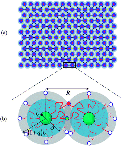 | ||
| Fig. 1 Network of cross-linked polymer grafted nanoparticles (PGNs) (a) graphical output from the simulation showing the initial configuration of the system for a corona height of q = 0.75. The core (dark blue region) is surrounded by a corona of grafted chains (blue and grey region). The reactive end groups on chains in the corona of neighboring PGNs form labile or permanent bonds, leading to the creation of the dual cross-linked network (b) schematic showing formation of bonds within the corona overlap region; the bonded chains are drawn in a solid red line and the red and green filled circles indicate the respective labile and permanent bonds. | ||
The interaction between two PGNs is modeled through a sum of interaction potentials and is given by Uint = Urep + Ucoh + Ulink. The first term characterizes the repulsive interactions between the coated nanoparticles. We assume that the grafted coronas are sufficiently thick that the rigid cores do not interact directly through the hard sphere repulsion, and the repulsion between the PGNs is due solely to the interaction between the corona chains that occurs when two PGNs come into close contact. At small corona overlaps, it is reasonable to assume that the actual repulsion between two PGNs is similar to that between two multi-arm star polymers that have the same size and same number of arms as the PGNs.21 (Notably, the repulsive forces obtained through molecular dynamics simulations of multi-arm star polymers containing a small core22 were found to be in quantitative agreement with theoretical predictions for the repulsion between star polymers.21) Hence, we describe the repulsion at the center-to-center distance of R through the effective pair potential proposed for the interactions between multi-arm star polymers:21
 | (1) |
The second term in the potential Uint describes the attractive cohesive interaction between the coated particles and chosen to have the following form:24
Ucoh(R) = −![[thin space (1/6-em)]](https://www.rsc.org/images/entities/char_2009.gif) C C![[thin space (1/6-em)]](https://www.rsc.org/images/entities/char_2009.gif) {1 + exp[(R − A)/B]}−1 {1 + exp[(R − A)/B]}−1 | (2) |
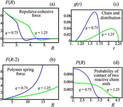 | ||
| Fig. 2 Effect of corona thickness, q, on pair interactions (blue and green lines denote q = 0.75 and 1.25 particles, respectively). (a) Repulsive–cohesive forces, F, between particles as a function of the separation distance, R. (b) Force exerted by a single bonded polymer chain, F, as a function of the separation distance, R. (c) Distribution of free ends in an isolated particle corona, g, as a function of distance from center of the particle, r. (d) Bond formation probability, P, in the corona overlap volume as a function of separation distance, R. | ||
The final term in the potential, Ulink, describes the attractive interaction between the particles linked by the bonded polymer arms. When functional groups at the chain ends of neighboring PGNs form a bond, then the nanoparticles are connected by a chain formed by joining the two interacting polymer arms (see Fig. 1b). These interconnecting polymer arms introduce an attractive interaction between the particles due to the spring-like entropic elasticity of the polymer chains. Consequently, the attractive force acting between the two bonded particles is given by the following equation:
Flink(r) = Nb![[thin space (1/6-em)]](https://www.rsc.org/images/entities/char_2009.gif) κ(r) κ(r)![[thin space (1/6-em)]](https://www.rsc.org/images/entities/char_2009.gif) ![[thin space (1/6-em)]](https://www.rsc.org/images/entities/char_2009.gif) r r | (3) |
| κ(r) = κ0{1 + 2[1 − r2(2L)−2]−2} | (4) |
In the above equation, 2L is the contour length of the chain formed by bonding two corona arms of length L. When the chain is deformed slightly so that the end-to-end distance r ≪ 2L, eqn (4) gives the spring constant of a Gaussian chain, i.e., κ(r) ≈ 3kBT![[thin space (1/6-em)]](https://www.rsc.org/images/entities/char_2009.gif) R0−2 ≡ 3κ0, where R02 = 4lpL is the mean-square end-to-end distance of the worm-like chain with the persistence length lp.25 The spring constant κ(r) increases (polymer chain stiffens) when the end-to-end distance r becomes comparable to the contour length of the chain 2L (see eqn (4)). Fig. 2b shows the polymer spring force as a function of r at the two values of corona thickness q indicated in the figure. It is seen that the force Flink(r) is a linear function of r at small separations between the particles, and then increases rapidly at large separations. At a given number of arms f, a larger corona thickness corresponds to longer corona arms (see below), so that the polymer spring force Flink is smaller and the chain stiffening takes place at larger inter-particle separations than those at a thinner corona (see Fig. 2b).
R0−2 ≡ 3κ0, where R02 = 4lpL is the mean-square end-to-end distance of the worm-like chain with the persistence length lp.25 The spring constant κ(r) increases (polymer chain stiffens) when the end-to-end distance r becomes comparable to the contour length of the chain 2L (see eqn (4)). Fig. 2b shows the polymer spring force as a function of r at the two values of corona thickness q indicated in the figure. It is seen that the force Flink(r) is a linear function of r at small separations between the particles, and then increases rapidly at large separations. At a given number of arms f, a larger corona thickness corresponds to longer corona arms (see below), so that the polymer spring force Flink is smaller and the chain stiffening takes place at larger inter-particle separations than those at a thinner corona (see Fig. 2b).
Above, we defined Nb to be the number of polymer chains formed between two PGNs by bonding the polymer arms. The value of Nb depends on the extent of overlap between the coronas of the nanoparticles, and on the kinetics of bond formation and rupture. The set of bonded arms are referred to as a link; in other words, each link in the network corresponds to multiple reformable bonds. To calculate Nb, we examine the kinetics of bond formation and rupture at three different hierarchies of interaction between the nanoparticles. First, we determine the kinetics of bond formation and rupture at the level of an individual bond. Second, we use geometric considerations to determine the number of chains encountered at a specific distance from the surface of the core. Third, we combine the information from the first and second levels with the distribution of bonding pairs that are located in the corona overlap volume to determine the evolution equation for the number of bonds as a function of separation distance.
At the individual bond level, we use the Bell model26–29 to describe the rupture and re-formation of bonds due to thermal fluctuations. In accordance with the Bell model, the rupture rate constant,k(p,l)r, is an exponential function of the force applied to the bond and is given by k(p,l)r = k(p,l)0rexp(γ0F), where k(p,l)0r = ν(p,l)exp(−U(p,l)0/kBT) is the rupture rate in the zero force limit that depends on the energy barrier U(p,l)0 separating the bound and the free states. For reversible bond formation in the zero force limit, the ratio of the formation to rupture rate constants is given by k(l)0f/k(l)0r = exp(U(l)0/kBT).27,28 In general, the rate constant of bond formation decreases under an applied force.29 The force due to chain extension, however, only affects the rate constants k(l)r and k(l)f at sufficiently large separations between a pair of polymer grafted nanoparticles. At the latter separations, the coronas do not overlap, so the total rate of labile bond formation is zero. Hence, for the sake of simplicity, we neglect the dependence of the rate constant of bond formation on force and consider it to be constant, k(l)0f. We note that it is only the labile bonds that can reform after breaking; the permanent bonds can only break.
The number of grafted chains available for linking a PGN to the neighboring particle located at the center-to-center distance R cannot exceed the number of chain ends that could be found in the overlap volume of the two coronas, Nmax(R). We estimate the value of Nmax by making the simplifying assumption that there is negligible distortion of the two coronas when they overlap. Then, purely geometric considerations yield the following expression:
 | (5) |
 | (6) |
 | (7) |
In order to calculate the probability of contact Pc(R), we introduce the chain end distribution function g(r), which is the probability distribution function for finding a chain end at the distance r from the center of the nanoparticle. The distribution function g(r) is normalized as
 | (8) |
 | (9) |
 | (10) |
Fig. 2c shows g(r) calculated for q = 0.75 and 1.25 as indicated in the figure. It is seen that the chain ends are distributed non-uniformly in the corona, with the maximal probability being located close to the corona outer surface at r = 1 + q. The exclusion zone near the nanoparticle surface at r = 1 is also clearly seen in Fig. 2c.
Finally, the probability of contact, Pc(R), was determined by the numerical integration indicated in eqn (9). The results of the numerical integration at the corona thicknesses of q = 0.75 and 1.25 are presented in Fig. 2d.
At a given nanoparticle radius of r0 and number of grafted arms f, the thickness of the corona H = q![[thin space (1/6-em)]](https://www.rsc.org/images/entities/char_2009.gif) r0 depends on the contour length L of the polymer arm. Self-consistent field theory provides the following equation that relates the corona thickness and arm length:30
r0 depends on the contour length L of the polymer arm. Self-consistent field theory provides the following equation that relates the corona thickness and arm length:30
| (H/H0)3(1 + 3q/4 + q2/5) = 1, | (11) |
H0 = 2π−2/3Lυ1/3(f![[thin space (1/6-em)]](https://www.rsc.org/images/entities/char_2009.gif) l2p/4π l2p/4π![[thin space (1/6-em)]](https://www.rsc.org/images/entities/char_2009.gif) r20)1/3. r20)1/3. | (12) |
The dynamics of the system is assumed to be in the overdamped regime, with the motion of each particle governed by the equation dx/dt = μ![[thin space (1/6-em)]](https://www.rsc.org/images/entities/b_char_2009.gif) Ftot, where μ is the mobility and
Ftot, where μ is the mobility and ![[thin space (1/6-em)]](https://www.rsc.org/images/entities/b_char_2009.gif) Ftot is the total force on the polymer grafted particle. The total force acting on a particle can be written as
Ftot is the total force on the polymer grafted particle. The total force acting on a particle can be written as ![[thin space (1/6-em)]](https://www.rsc.org/images/entities/b_char_2009.gif) Ftot = −∂Uint/∂x + Fext, where Fext is the external force acting on the edge particles of the particle array (see Fig. 1b). This equation is solved numerically in two steps since the polymer spring force (within the expression for
Ftot = −∂Uint/∂x + Fext, where Fext is the external force acting on the edge particles of the particle array (see Fig. 1b). This equation is solved numerically in two steps since the polymer spring force (within the expression for ![[thin space (1/6-em)]](https://www.rsc.org/images/entities/b_char_2009.gif) Ftot) in the dynamic equation depends on the number of bonds between particles and consequently, on the evolution of the chemical kinetics given by eqn (6). In the first step, we determine the number of bonds at any given time, Nb(t), by numerically solving eqn (6) through an explicit Euler scheme with a time step of Δt = 10−2T0, where T0 is the unit of time in the simulation (see Table 1). Note that the numerical evolution of eqn (6) yields a real number, whereas the number of bonds Nb(t) should take discrete integer values. In order to determine the integer value, we compare the fractional part of the numerical result, {Nb(t)}, with a random number ξ distributed uniformly between 0 and 1. If {Nb(t)} < ξ, then we truncate the result; otherwise, we increment the integer part of the result by 1. In the second step, we use this value for the number of bonds to calculate the spring force (see eqn (3)) in the dynamic equation and integrate numerically the resulting equation using a fourth-order Runge–Kutta algorithm with a time step of Δt = 10−2T0.
Ftot) in the dynamic equation depends on the number of bonds between particles and consequently, on the evolution of the chemical kinetics given by eqn (6). In the first step, we determine the number of bonds at any given time, Nb(t), by numerically solving eqn (6) through an explicit Euler scheme with a time step of Δt = 10−2T0, where T0 is the unit of time in the simulation (see Table 1). Note that the numerical evolution of eqn (6) yields a real number, whereas the number of bonds Nb(t) should take discrete integer values. In order to determine the integer value, we compare the fractional part of the numerical result, {Nb(t)}, with a random number ξ distributed uniformly between 0 and 1. If {Nb(t)} < ξ, then we truncate the result; otherwise, we increment the integer part of the result by 1. In the second step, we use this value for the number of bonds to calculate the spring force (see eqn (3)) in the dynamic equation and integrate numerically the resulting equation using a fourth-order Runge–Kutta algorithm with a time step of Δt = 10−2T0.
| Dimensional units | |
|---|---|
| Length: nanoparticle radius | r 0 = 50 nm |
| Time, t | T 0 = 1.41 × 10⁻² s |
| Velocity, v | v 0 = r0T0−1 = 3.55 μm s−1 |
| Force, F | F 0 = 2.98 pN |
| Toughness, W | F 0 r 0 = 89.74 kJ mol−1 |
| Bond parameters | Weaker labile bond | Stronger labile bond | Permanent bond |
|---|---|---|---|
| Bond energy, U0 | 33![[thin space (1/6-em)]](https://www.rsc.org/images/entities/char_2009.gif) kBT kBT |
39![[thin space (1/6-em)]](https://www.rsc.org/images/entities/char_2009.gif) kBT kBT |
45![[thin space (1/6-em)]](https://www.rsc.org/images/entities/char_2009.gif) kBT kBT |
| Rupture rate at zero force, k0r | 6.555 × 10⁻⁴T0−1 | 1.625 × 10⁻⁶T0−1 | 4.028 × 10⁻⁹T0−1 |
| Formation rate, k0f | 30T0−1 | 30T0−1 | 0 |
| Bond sensitivity, γ0 | 6F0−1 | 6F0−1 | 6F0−1 |
| Characteristics of polymer grafted nanoparticle (PGN) | Corona thickness H = 0.75![[thin space (1/6-em)]](https://www.rsc.org/images/entities/char_2009.gif) r0 r0 |
Corona thickness H = 1.25![[thin space (1/6-em)]](https://www.rsc.org/images/entities/char_2009.gif) r0 r0 |
|---|---|---|
| Kuhn length, lp | 1 nm | 1 nm |
| Excluded volume parameter, υ | 0.25 | 0.25 |
| Number of grafted arms, f | 156 | 156 |
| Arm contour length, L | 8.89![[thin space (1/6-em)]](https://www.rsc.org/images/entities/char_2009.gif) r0 r0 |
16.35![[thin space (1/6-em)]](https://www.rsc.org/images/entities/char_2009.gif) r0 r0 |
| Chain spring constant, κ0 | 7.81 × 10⁻²F0r0−1 | 4.25 × 10⁻²F0r0−1 |
| Repulsion parameter σ | 3.02![[thin space (1/6-em)]](https://www.rsc.org/images/entities/char_2009.gif) r0 r0 |
3.88![[thin space (1/6-em)]](https://www.rsc.org/images/entities/char_2009.gif) r0 r0 |
| Cohesion parameter A | 1.15![[thin space (1/6-em)]](https://www.rsc.org/images/entities/char_2009.gif) σ σ |
1.15![[thin space (1/6-em)]](https://www.rsc.org/images/entities/char_2009.gif) σ σ |
| B | 0.08![[thin space (1/6-em)]](https://www.rsc.org/images/entities/char_2009.gif) σ σ |
0.08![[thin space (1/6-em)]](https://www.rsc.org/images/entities/char_2009.gif) σ σ |
| C | 60![[thin space (1/6-em)]](https://www.rsc.org/images/entities/char_2009.gif) kBT kBT |
60![[thin space (1/6-em)]](https://www.rsc.org/images/entities/char_2009.gif) kBT kBT |
| Mobility of PGN, μ | 0.57![[thin space (1/6-em)]](https://www.rsc.org/images/entities/char_2009.gif) v0F0−1 v0F0−1 |
0.44![[thin space (1/6-em)]](https://www.rsc.org/images/entities/char_2009.gif) v0F0−1 v0F0−1 |
| Pulling velocity, v | 0.001![[thin space (1/6-em)]](https://www.rsc.org/images/entities/char_2009.gif) v0 and 0.005 v0 and 0.005![[thin space (1/6-em)]](https://www.rsc.org/images/entities/char_2009.gif) v0 v0 |
0.001![[thin space (1/6-em)]](https://www.rsc.org/images/entities/char_2009.gif) v0 v0 |
The initial state of the system is generated using the following five-step procedure. In the first step, the nanoparticles are placed in an array such that their centers are separated by a horizontal spacing of 1.8![[thin space (1/6-em)]](https://www.rsc.org/images/entities/char_2009.gif) (1 + q) and a vertical spacing of 1.62
(1 + q) and a vertical spacing of 1.62![[thin space (1/6-em)]](https://www.rsc.org/images/entities/char_2009.gif) (1 + q), with a horizontal offset position of 0.855 (1 + q) between adjacent rows. In the second step, we hold the sample in the initial configuration for 4000 T0 units of time to allow for the formation of the labile bonds. In the third step, we equilibrate the sample for a time 6000 T0, during which the stressed labile bonds are broken and new bonds are formed between the adjacent PGNs according to eqn (6). In the fourth step, we establish the permanent bonds with the probability P. In this step, if two particles are linked with Nb bonds, then with the probability P, one of the bonds is designated as “permanent”, so that the two particles become linked with (Nb − 1) labile bonds and one permanent bond. In this fifth step, the resultant sample composed of a dual-network of permanent and labile bonds is equilibrated for 104T0 and then subject to tensile deformation by stretching at a constant velocity of 3.55 or 17.75 nm s−1. The latter values of velocity are similar to that used in single molecule pulling experiments.33
(1 + q), with a horizontal offset position of 0.855 (1 + q) between adjacent rows. In the second step, we hold the sample in the initial configuration for 4000 T0 units of time to allow for the formation of the labile bonds. In the third step, we equilibrate the sample for a time 6000 T0, during which the stressed labile bonds are broken and new bonds are formed between the adjacent PGNs according to eqn (6). In the fourth step, we establish the permanent bonds with the probability P. In this step, if two particles are linked with Nb bonds, then with the probability P, one of the bonds is designated as “permanent”, so that the two particles become linked with (Nb − 1) labile bonds and one permanent bond. In this fifth step, the resultant sample composed of a dual-network of permanent and labile bonds is equilibrated for 104T0 and then subject to tensile deformation by stretching at a constant velocity of 3.55 or 17.75 nm s−1. The latter values of velocity are similar to that used in single molecule pulling experiments.33
In the ensuing simulations, we consider a particle of core radius r0 = 50 nm with f = 156 polymer chains grafted onto its surface. (As noted in Table 1, the Kuhn length of these grafted chains is lp = 1 nm.) The value of f was chosen to satisfy the assumption that the corona chains are in the semi-dilute regime; this constraints the value of f to f1/2 ≤ υ![[thin space (1/6-em)]](https://www.rsc.org/images/entities/char_2009.gif) r0
r0![[thin space (1/6-em)]](https://www.rsc.org/images/entities/char_2009.gif) lp−1.31,32 The value of f is used to determine the strength of repulsion and extent of bond formation between any two interacting particles through eqn (1) and (5), respectively.
lp−1.31,32 The value of f is used to determine the strength of repulsion and extent of bond formation between any two interacting particles through eqn (1) and (5), respectively.
The cohesive interaction in eqn (2) with A = 1.15σ, B = 0.08σ, and C = 60kBT counters the repulsive forces at the corona edge. At the chosen values of the pseudo-potential parameters A, B, and C, the equilibrium distance between an isolated pair of PGNs without bonds corresponds to ∼1% corona overlap. The overlap increases in the presence of bonds. For example, at equilibrium, a pair of PGNs with the corona thickness q = 1.25 form ∼8 labile bonds of energy U(l)0 = 39![[thin space (1/6-em)]](https://www.rsc.org/images/entities/char_2009.gif) kBT, and exhibit ∼10% corona overlap. It is important to note that if the cohesive interactions are not taken into account, the equilibrium state of the pair of PGNs corresponds to no corona overlap and no labile bonds.
kBT, and exhibit ∼10% corona overlap. It is important to note that if the cohesive interactions are not taken into account, the equilibrium state of the pair of PGNs corresponds to no corona overlap and no labile bonds.
The motion of the particle in the overdamped regime is determined using the mobility computed as the inverse of Stokes drag, μ = [6πη![[thin space (1/6-em)]](https://www.rsc.org/images/entities/char_2009.gif) r0(1 + q)]−1, on a particle of radius r0(1 + q) in a viscous fluid of viscosity η = 0.894 Pa s (viscosity of glycerol). For convenience, all the parameters used in the simulations are collected in Table 1.
r0(1 + q)]−1, on a particle of radius r0(1 + q) in a viscous fluid of viscosity η = 0.894 Pa s (viscosity of glycerol). For convenience, all the parameters used in the simulations are collected in Table 1.
In simulating bond kinetics, we fix the bond energy of the permanent bonds to be U(p)0 = 45![[thin space (1/6-em)]](https://www.rsc.org/images/entities/char_2009.gif) kBT and vary P in the range 0 ≤ P ≤ 1. Note that at P = 1, each pair of neighboring nanoparticles is interconnected by one permanent bond and at P = 0, there are no permanent bonds in the sample; for example, if P = 0.6, then, 60% of the neighboring pairs are connected by a permanent bond. (Note that the latter permanent bonds are randomly distributed throughout the sample.) We examine the two cases of labile bond energy of U(l)0 = 33
kBT and vary P in the range 0 ≤ P ≤ 1. Note that at P = 1, each pair of neighboring nanoparticles is interconnected by one permanent bond and at P = 0, there are no permanent bonds in the sample; for example, if P = 0.6, then, 60% of the neighboring pairs are connected by a permanent bond. (Note that the latter permanent bonds are randomly distributed throughout the sample.) We examine the two cases of labile bond energy of U(l)0 = 33![[thin space (1/6-em)]](https://www.rsc.org/images/entities/char_2009.gif) kBT and 39
kBT and 39![[thin space (1/6-em)]](https://www.rsc.org/images/entities/char_2009.gif) kBT. We also consider the two cases of corona thickness of q = 0.75 and 1.25, and the two cases of stretching velocity of v = 0.001 and 0.005 (see Table 1). As noted above, each link in the network corresponds to multiple reformable bonds, and may contain one permanent bond. The rates of rupture and formation of bonds within the links varies as a function of corona overlap and the nature of the bonds (labile/permanent). The links stretch due to an applied deformation with the maximum extent of the stretching corresponding to the contour length of the grafted chains. When the links are stretched, the force exerted on the bonds in the link increases with separation and facilitates bond rupture. In the absence of an external force, the system exhibits a steady-state, where the rupture of labile bonds is balanced by bond formation, thus leading to the existence of a finite number of labile bonds in the overlap region between particles. Note that the model assumes that no bond formation is possible in the absence of overlap, so that Nb = 0 in the steady state at no overlap. The assumption concerning the absence of bond formation beyond the corona is equivalent to assuming an immediate retraction of arms upon bond rupture. Finally, we note that eqn (6) describes dynamics of the number of bonds in any situation, with or without the corona overlap.
kBT. We also consider the two cases of corona thickness of q = 0.75 and 1.25, and the two cases of stretching velocity of v = 0.001 and 0.005 (see Table 1). As noted above, each link in the network corresponds to multiple reformable bonds, and may contain one permanent bond. The rates of rupture and formation of bonds within the links varies as a function of corona overlap and the nature of the bonds (labile/permanent). The links stretch due to an applied deformation with the maximum extent of the stretching corresponding to the contour length of the grafted chains. When the links are stretched, the force exerted on the bonds in the link increases with separation and facilitates bond rupture. In the absence of an external force, the system exhibits a steady-state, where the rupture of labile bonds is balanced by bond formation, thus leading to the existence of a finite number of labile bonds in the overlap region between particles. Note that the model assumes that no bond formation is possible in the absence of overlap, so that Nb = 0 in the steady state at no overlap. The assumption concerning the absence of bond formation beyond the corona is equivalent to assuming an immediate retraction of arms upon bond rupture. Finally, we note that eqn (6) describes dynamics of the number of bonds in any situation, with or without the corona overlap.
III. Results and discussion
An important aspect of our approach to modeling the mechanical behavior of the dual cross-linked networks is that we combine known features of the interaction between two PGNs21–25,30 with the non-equilibrium kinetics of bond rupture and formation described by the Bell model.26–29 Using this new approach, we analyze the materials' mechanical performance by applying a tensile deformation to a sample at constant velocity (strain-controlled deformation), and determine the resulting force F on the sample and the number of bonds per particle as functions of strain, ε.The strain ε is calculated as the ratio of the extension of the sample to the original length. The ductility of the sample is characterized by the strain at break, εb, which is determined as the strain at which the force required for deformation drops as the sample fractures. The work done by the external force to fracture the sample (work-to-break) is a measure of the toughness of the material. In the macroscopic, continuum limit, the toughness is calculated as the work-to-break per unit volume of the undeformed sample.34,35 Because, however, our simulations are performed at the mesoscopic level, it is more appropriate to define toughness as the work-to-break per one particle. Hence, the value of toughness, W, is determined by integrating the force-extension curve, and dividing the resulting work by the number of nanoparticles in the sample, NPGN.
Here, each sample is composed of NPGN = 180 particles, which are initially arranged in 12 rows, with 15 particles in each row (see Methodology). To quantify the properties of the material formed from the dual cross-linked PGNs, eight independent runs are performed at each set of specified model parameters, and then the Weibull statistics36 is employed to determine the ductility and toughness.
A. Effects of the dual crosslinking on mechanical properties of PGNs
The behavior of the dual cross-linked PGNs depends on the strength of the labile bonds and the fraction of permanent bonds within the network. The energies of the labile bonds chosen here are such that for the weaker labile bonds (U(l)0 = 33![[thin space (1/6-em)]](https://www.rsc.org/images/entities/char_2009.gif) kBT), the bond rupture rate is of the same order of magnitude as the tensile deformation strain rate, whereas for the stronger labile bonds (U(l)0 = 39
kBT), the bond rupture rate is of the same order of magnitude as the tensile deformation strain rate, whereas for the stronger labile bonds (U(l)0 = 39![[thin space (1/6-em)]](https://www.rsc.org/images/entities/char_2009.gif) kBT), the rupture rate is approximately two orders of magnitude lower than the strain rate. As described in the Methodology, for 0 < P ≤ 1, the inter-particle links encompass a single permanent bond in addition to the existing labile bonds. The energy of the permanent bond is taken to be U(p)0 = 45
kBT), the rupture rate is approximately two orders of magnitude lower than the strain rate. As described in the Methodology, for 0 < P ≤ 1, the inter-particle links encompass a single permanent bond in addition to the existing labile bonds. The energy of the permanent bond is taken to be U(p)0 = 45![[thin space (1/6-em)]](https://www.rsc.org/images/entities/char_2009.gif) kBT, which corresponds to a bond rupture rate that is approximately five orders of magnitude lower than the strain rate.
kBT, which corresponds to a bond rupture rate that is approximately five orders of magnitude lower than the strain rate.
We first examine the material properties of dual cross-linked PGNs that have a corona thickness of q = 0.75 and are subjected to a strain-controlled tensile deformation applied at a constant velocity of v = 0.001 (corresponding to roughly 3.55 nm s−1). Fig. 3 presents the strain at break εb (Fig. 3a) and toughness W (Fig. 3b) of the samples, which contain the weaker (curves 1) and stronger (curves 2) labile bonds, as functions of the fraction of permanent bonds P. The data points and error bars shown in Fig. 3 were obtained by averaging over eight independent simulation runs (see above).
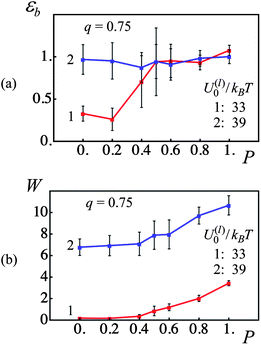 | ||
| Fig. 3 Effect of fraction of permanent bonds, P, and labile bond energy, U(l)0/kBT, on strain at break, εb, and toughness, W (red and blue lines denote U(l)0/kBT = 33 and 39, respectively). (a) Strain at break, εb, as a function of fraction of permanent bonds, P. (b) Toughness, W, as a function of fraction of permanent bonds, P. | ||
As can be seen from Fig. 3, the presence of the permanent cross-links is crucial for optimal mechanical performance if the labile bonds are weak. At lower fractions of permanent bonds, the PGNs having the weaker labile bonds exhibit a very low toughness (see curve 1 in Fig. 3b at 0 < P ≤ 0.4) and a strain at break of about 0.25 (see curve 1 in Fig. 3a at P < 0.2). At higher values of P, the permanent bonds form an elastic skeleton in the latter system that leads to a notable improvement in the material properties. Namely, ductility of the system having the weaker labile bonds increases to εb ≈ 1.0 at P ≥ 0.5 (Fig. 3a, curve 1), and toughness of the system exhibits an increase from W ∼ 1 at P = 0.5 to W ≈ 3.5 at P = 1 (Fig. 3b, curve 1).
In contrast, the PGNs linked with the stronger labile bonds produce a ductile, tough material even in the absence of the permanent bonds, i.e., at P = 0 (see Fig. 3a and b, curves 2). Introduction of permanent bonds into the system does not affect the strain at break, which remains at εb ≈ 1.0 for 0 ≤ P ≤ 1 as seen in Fig. 3a, curve 2. The permanent bonds, however, improve the toughness of the material; namely, W ≈ 7 at P = 0 is increased to W ≈ 11 at P = 1 (Fig. 3b, curve 2).
It is noteworthy that at P = 1, the toughness of the sample with the stronger labile bonds is three times greater than that of the sample with the weaker labile bonds (Fig. 3b), whereas the strain at break is the same in the two systems (Fig. 3a). This behavior, as well as the overall effect of dual cross-linking on the mechanical properties of PGNs, can be better understood as we analyze the materials' tensile behavior in more detail in the following discussion.
Fig. 4a and b show the force–strain curves for the samples having the weaker (U(l)0 = 33![[thin space (1/6-em)]](https://www.rsc.org/images/entities/char_2009.gif) kBT) and stronger (U(l)0 = 39
kBT) and stronger (U(l)0 = 39![[thin space (1/6-em)]](https://www.rsc.org/images/entities/char_2009.gif) kBT) labile bonds at the fractions of permanent bonds of P = 0, 0.6 and 1. Each curve corresponds to a single run of the simulations for samples with a corona thickness of q = 0.75 and a tensile deformation that is applied at a constant velocity of v = 0.001. The arrows pointing downwards indicate sample breakage. Notably, the data in Fig. 3 on ductility and toughness were obtained by analyzing force–strain curves similar to those in Fig. 4a and b.
kBT) labile bonds at the fractions of permanent bonds of P = 0, 0.6 and 1. Each curve corresponds to a single run of the simulations for samples with a corona thickness of q = 0.75 and a tensile deformation that is applied at a constant velocity of v = 0.001. The arrows pointing downwards indicate sample breakage. Notably, the data in Fig. 3 on ductility and toughness were obtained by analyzing force–strain curves similar to those in Fig. 4a and b.
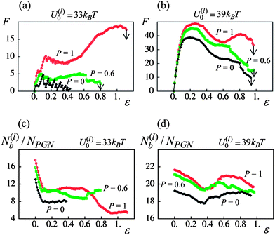 | ||
| Fig. 4 Effect of fraction of permanent bonds, P, on mechanical response of network. (a) Force(F)–strain(ε) curves at P = 0, 0.6 and 1 (black, green and red curves, respectively) for U(l)0/kBT = 33. (b) Force(F)–strain(ε) curves at P = 0, 0.6 and 1 for U(l)0/kBT = 39. (c) Number of labile bonds/particle, N(l)b/NPGN, as a function of strain, ε, at P = 0, 0.6 and 1 for U(l)0/kBT = 33. (d) Number of labile bonds/particle, N(l)b/NPGN, as a function of strain, ε, at P = 0, 0.6 and 1 for U(l)0/kBT = 39. | ||
Fig. 4a and b indicate that the behavior of the dual cross-linked PGNs under tensile deformation is similar to that of ductile polymeric materials.34,35 Namely, at the smaller strains, dual cross-linked PGNs behave as elastic materials. At a strain of about 15–20%, the samples reach a yield point, after which the force F decreases (Fig. 4a and b). (Recall that this force represents the resistance of the material to deformation.) After the yield point, the material exhibits two distinct behaviors, which depend quite markedly on P. Specifically, the force can reach a local minimum and then increases before the breakage, as seen in at Fig. 4a at P = 0.6 and 1 and in Fig. 4b at P = 1. The latter force–strain behavior is characteristic of polymeric materials that exhibit cold-drawing and necking.34,35 Alternatively, the force can continue to decrease until the sample breaks, as seen in Fig. 4a at P = 0 and Fig. 4b at P = 0 and 0.6.
Fig. 4a and b also reveal the significant effect that the energy of labile bonds has on the mechanical performance of dual cross-linked PGNs. The weaker labile bonds cannot withstand deformation without the presence of permanent bonds as the force F varies around some low value (see Fig. 4a, P = 0). The sample becomes elastic only after a sufficient amount of permanent bonds is added, so that at P = 1, the yield strain and force are about 15% and 10, respectively (Fig. 4a). In contrast, at P = 0, the sample having the stronger labile bonds exhibits the yield point at 20% strain, and the force at yield is of F ≈ 38 (Fig. 4b). Introducing the permanent cross-links to the PGNs linked by the stronger labile bonds increases the yield force up to F ≈ 50 at P = 1, and modifies the post-yield behavior so that the sample exhibits quite pronounced cold-drawing/necking at P = 1 (Fig. 4b).
In the course of sample deformation, the rupture of stressed labile bonds takes place simultaneously with the formation of new bonds within the overlapped coronas. Fig. 4c and d show the respective numbers of labile bonds per particle in the systems having the weaker and stronger labile bonds as functions of the strain ε. Initially, N(l)b drops upon the tensile deformation of a sample (cf.Fig. 4a–d). Then, after the sample yields, the number of bonds exhibits an increase; the latter behavior is especially noticeable in the system having the stronger labile bonds (Fig. 4d). The increase in N(l)b indicates that the material is capable of self-healing, particularly in the sample with the stronger labile bonds.
Fig. 4c and d show that the number of labile bonds in the dual cross-linked PGNs is quite large. Specifically, at a strain of 50% and P = 1, there are about 11 labile bonds per one particle in the case of weaker bonds (Fig. 4c), and about 20 labile bonds per particle in the case of stronger bonds (Fig. 4d). Besides the labile bonds, all the PGNs are linked by the permanent bonds at P = 1. Fig. 5 reveals that the relative contributions of the labile and permanent bonds to the force F are different and depend on the strength of labile bonds. In Fig. 5a, the force–strain curves for the dual cross-linked PGNs at P = 1 are plotted together with a curve for a system labeled “permanent only” where the links between particles are comprised solely of a single permanent bond. The latter system was prepared using the same procedure as describe above, but the formation of the labile bonds was prohibited both initially and in the course of deformation.
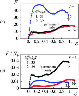 | ||
| Fig. 5 Effect of labile bond energy, U(l)0/kBT, at P = 1. (a) Force(F)–strain(ε) curves for U(l)0/kBT = 33, 39 and in absence of labile bonds (red, blue and black curves, respectively). (b) Normalized force per bond, F/Nb, versus strain, ε, curves for U(l)0/kBT = 33, 39 and in absence of labile bonds. | ||
It is evident from Fig. 5a that the weaker labile bonds do not contribute to the force as curve 1 and the “permanent only” plots effectively coincide. On the other hand, the contribution of the stronger labile bonds to F is quite remarkable. Not all the stronger labile bonds, however, contribute to the force. The latter observation follows from Fig. 5b, which shows the same force–strain curves as in Fig. 5a but after normalization by the total number of bonds in the system, F/Nb. As can be seen in Fig. 5b, the force per one bond is lower in the dual cross-linked systems than that in the system containing only the permanent bonds.
Fig. 5 indicates that the strain at break is controlled mostly by the permanent bonds. Indeed, after averaging over 8 runs, the values of εb for the systems shown in Fig. 5 were essentially equal. Namely, εb = 0.95 ± 0.04 in the case of permanent bonds only, and εb = 1.07 ± 0.06 and 1.0 ± 0.08 in the respective cases of weaker and stronger labile bonds at P = 1. These observations help explain the P = 1 curves in Fig. 3, which show that the strain at break is approximately the same in the two systems involving labile bonds.
We can obtain further physical insight into the data in Fig. 5 by examining snapshots from the simulations of the materials undergoing tensile deformation. Fig. 6 and 7 show samples containing the weaker and stronger labile bonds at P = 1, respectively, for strains of ε = 0.3, 0.58 and 0.95. These snapshots show just the particles and the labile bonds; for clarity, the permanent bonds are not displayed. The number of labile bonds in a link is indicated by the color code in Fig. 6d.
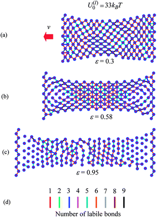 | ||
| Fig. 6 Snapshot of sample with weaker labile bonds with P = 1 at strains (a) ε = 0.30, (b) ε = 0.58 and (c) ε = 0.95. The line colors indicate the number of labile bonds in the link. | ||
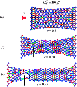 | ||
| Fig. 7 Snapshot of sample with stronger labile bonds with P = 1 at strains (a) ε = 0.30, (b) ε = 0.58 and (c) ε = 0.95. The line colors indicate the number of labile bonds in the link. | ||
Fig. 6 reveals that the weaker labile bonds break easily in the direction of the tensile deformation; as can be seen, there are only a few horizontal links even at the lowest strain shown, ε = 0.3 (Fig. 6a). This tensile deformation is accompanied by the contraction of the sample in the transverse direction. As a result, the newly formed labile bonds are normal to the direction of stretching (Fig. 6b and c), so they do not contribute to the tensile force. At the higher strain of ε = 0.95, the surviving weaker labile bonds form the prominent vertical “stripes” seen in Fig. 6c.
The total number and distribution of stronger labile bonds in Fig. 7 are quite different from the picture seen in Fig. 6. In contrast to Fig. 6a, Fig. 7a reveals that there are still many labile bonds along the stretching direction at ε = 0.3. The latter bonds give rise to the large tensile forces observed in Fig. 5a in the case of stronger labile bonds. Further deformation results in a decrease in the number of labile bonds in the direction of stretching and in the formation of labile bonds in the normal direction (see Fig. 7b). At the higher strain of ε = 0.95, the network formed by the stronger labile bonds is still dense (Fig. 7b) relative to that formed by the weaker labile bonds (Fig. 6c).
Finally, we note that samples having the weaker and stronger labile bonds exhibit different modes of failure. In the case of the weaker bonds, the sample fractures perpendicular to the direction of stretching (not shown). The sample having the stronger labile bonds breaks due to the formation and growth of a void, as indicated by the arrows in Fig. 7b and c.
B. Effects of corona thickness
The interaction forces between the cross-linked PGNs and the bond formation within the corona depend on the corona thickness, q. At a constant grafting density (0.005 chains per nm2), the value of q is controlled by the contour length of the grafted polymer chains, L. Here, we examine how a variation in the corona thickness affects the response of the materials to a tensile deformation that is applied at a constant strain rate of v = 0.001 (3.55 nm s−1).Fig. 8 shows a comparison of the strain at break εb and toughness W for samples prepared from PGNs having a corona thickness of q = 0.75 (curves 1 in Fig. 8) and 1.25 (curves 2 in Fig. 8). At the given grafting density (see above), the latter values of q correspond to chain lengths of L ≈ 8.88 and 16.3, respectively. Recall that the radius of the nanoparticles, r0, is used as the unit of length.
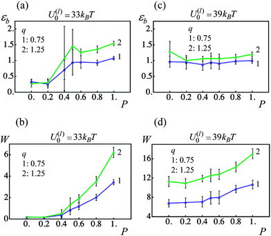 | ||
| Fig. 8 Effect of fraction of permanent bonds, P, and corona thickness, q, on strain at break, εb, and toughness, W (blue and green lines denote q = 0.75 and 1.25 samples, respectively). (a) Strain at break, εb, as a function of fraction of permanent bonds, P, for U(l)0/kBT = 33. (b) Toughness, W, as a function of fraction of permanent bonds, P, for U(l)0/kBT = 33. (c) Strain at break, εb, as a function of fraction of permanent bonds, P, for U(l)0/kBT = 39. (d) Toughness, W, as a function of fraction of permanent bonds, P, for U(l)0/kBT = 39. | ||
For the material with the weaker labile bonds, both the strain at break and the toughness of the sample increases with an increase in q at P > 0.6 (see Fig. 8a and b). Notably, at P = 1, the ductility is enhanced by approximately 40% and the toughness is increased by a factor of 1.8. The plots in Fig. 9 provide insight into factors contributing to this behavior. In particular, Fig. 9a shows that at P = 1 after the yield point, the force required to strain the sample is smaller for the larger corona thickness. The latter behavior occurs because a larger q corresponds to longer chains, so that the chain stiffening takes place at larger inter-particle separations than those at a thinner corona (see Fig. 2b). In other words, the polymer spring force Flink is smaller for a given inter-particle separation for the longer corona than the thinner one (see eqn (4)). Consequently, the q = 1.25 material can be strained to a greater extent than the q = 0.75 sample (note the arrows in Fig. 9 pointing to the respective values of εb), i.e., the sample with the higher corona thickness is more ductile.
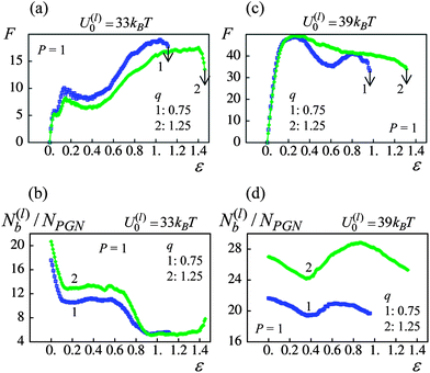 | ||
| Fig. 9 Effect of corona thickness at P = 1 on network response (blue and green lines denote q = 0.75 and 1.25 samples, respectively (a) force(F)–strain(ε) curves for U(l)0/kBT = 33. (b) Number of labile bonds/particle, N(l)b/NPGN, as a function of strain, ε, for U(l)0/kBT = 33. (c) Force(F)–strain(ε) curves for U(l)0/kBT = 39. (d) Number of labile bonds/particle, N(l)b/NPGN, as a function of strain, ε, for U(l)0/kBT = 39. | ||
It is noteworthy that in the U(l)0 = 33kBT samples, the number of labile bonds per particle, N(l)b/NPGN, does not increase considerably at the larger q (see Fig. 9b). Although the overlap between the coronas is greater at the larger q (see Fig. 2d), the high rate of rupture of these weaker labile bonds prevents a notable increase in the number of newly formed bonds. Furthermore, the number of bonds per particle is approximately the same for both values of q at 100% strain (see Fig. 9b). Hence, the observed increase in toughness (Fig. 8b) is primarily due to the increase in ductility. (Recall that here toughness is measured as the work-to-break per one particle.)
Fig. 10 provides further insight into the behavior of the samples having the weaker labile bonds, revealing that the increase in the strain at break with an increase in the corona thickness is primarily due to the delayed breakage of the permanent bonds. Fig. 10a shows the rates of a single bond breakage, −dp/dt, as function of strain ε calculated according to eqn (6) and (7) for a system of two PGNs, which are moved apart with the constant velocity of v = 0.001. The dashed and solid lines correspond to the corona thicknesses of q = 0.75 and 1.25, respectively. Fig. 10a shows that the increase in the corona thickness (chain length) has very little effect on the rate of breakage of the weaker labile bonds (red lines), whereas the permanent bonds within the thicker corona break at a notably larger strain (black lines).
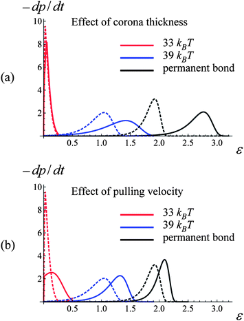 | ||
| Fig. 10 Effect of corona thickness, q, and pulling velocity, v, on bond rupture rate, −dp/dt, at bond energies U(l)0/kBT = 33, 39 and 45 (red, blue and black curves, respectively). (a) Bond rupture rate(−dp/dt)–strain(ε) curves for q = 0.75 and 1.25 (dashed and solid lines, respectively). (b) Bond rupture rate(−dp/dt)–strain(ε) curves for v = 0.001 and 0.005 (dashed and solid lines, respectively). | ||
For samples encompassing the stronger labile bonds (U(l)0 = 39kBT), the strain at break εb shows no statistically significant dependence on the corona thickness in the range 0 ≤ P ≤ 1 as seen in Fig. 8c. However, the PGNs having the thicker corona of q = 1.25 exhibit a greater toughness than those at q = 0.75 over the entire range of P. It is seen in Fig. 8d that the toughness W increases by a factor of 1.6 with the increase in q. The force–strain curves presented in Fig. 9c show that increasing q to 1.25 does not lead to a decrease in the force F for these more strongly bound materials; this is in contrast to the samples having the weaker labile bonds (Fig. 9a). Before the yield point, the curves for the different q are quite similar (Fig. 9c). After yielding, the force F in the sample with the thicker corona (curve 2 in Fig. 9c) decreases monotonously until the breakage, i.e., exhibits the behavior characteristic for a purely ductile material without cold drawing/necking seen at q = 0.75 (curve 1 in Fig. 9c).
The observed transition of the cross-linked PGNs to the purely ductile behavior at q = 1.25 (no necking) (Fig. 9c) could be attributed to the enhanced formation of labile bonds between particles having the thicker corona, as seen in Fig. 9d. The observed increase in N(l)b/NPGN is due to: (1) a greater corona overlap at q = 1.25 that facilitates contacts between chain ends (see Fig. 2d), and (2) the delayed rupture of the stronger labile bonds within the thicker corona. The latter behavior is evident from Fig. 10a, which shows that in a system of two PGNs, the stronger labile bonds at q = 1.25 (blue solid curve) break at a considerably larger strain than those at q = 0.75 (blue dashed line). The increase in N(l)b/NPGN necessitates greater work to break the sample and hence, leads to a greater toughness, as seen in Fig. 8d. (The enhanced bond formation also contributes to the slightly larger value of εb at the greater q for P = 1.)
C. Effects of strain rate
The mechanical properties of elastomers are known to depend on the deformation rate owing to the viscoelastic relaxation of polymer chains.35 The dual cross-linked PGNs exhibit an additional, unique mechanism of relaxation, which is due to the rupture and formation of the labile bonds. Variations in the strain rate could alter the mechanical response of the system of labile bonds especially when the rate of rupture is force-dependent. The latter is illustrated in Fig. 10b, which shows the rate of a single bond rupture, −dp/dt, upon pulling apart two PGNs at the two different velocities. The dashed and solid lines in Fig. 10b correspond to the velocities of v = 0.001 and 0.005, respectively, and color of a line denotes the bond energy as indicated in the figure. It is seen in Fig. 10b that the bonds rupture at larger strains as the velocity of pulling increases.We examine how variations in the strain rate affect the behavior of the PGN samples, which encompass the weaker (U(l)0 = 33kBT) and stronger (U(l)0 = 39kBT) labile bonds at the fraction of permanent bonds 0 ≤ P ≤ 1 and the corona thickness of q = 0.75. For this purpose, the samples are subjected to the tensile deformation at the constant pulling velocities of v = 0.001 (3.55 nm s−1) and v = 0.005 (17.75 nm s−1). The results of computer simulations are summarized in Fig. 11, which shows the strain at break εb and toughness W of the samples, and the labels “1” and “2” denote data obtained at the lower and higher velocity, respectively.
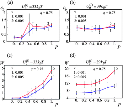 | ||
| Fig. 11 Effect of fraction of permanent bonds, P, and pulling velocity, v, on strain at break, εb, and toughness, W (blue and red lines denote pulling velocities v = 0.001 and 0.005, respectively). (a) Strain at break, εb, as a function of fraction of permanent bonds, P, for U(l)0/kBT = 33. (b) Strain at break, εb, as a function of fraction of permanent bonds, P, for U(l)0/kBT = 39. (c) Toughness, W, as a function of fraction of permanent bonds, P, for U(l)0/kBT = 33. (d) Toughness, W, as a function of fraction of permanent bonds, P, for U(l)0/kBT = 39. | ||
Fig. 11 shows that at the given parameters, the strain rate has no considerable effect on the ultimate tensile strains εb in the PGNs having the weaker (Fig. 11a) and stronger (Fig. 11b) labile bonds. However, an increase in the strain rate results in an increase in the toughness W of the samples, and the observed enhancement of toughness depends on the strength of labile bonds (Fig. 11c and d).
For the samples having the weaker labile bonds, there is no statistically significant effect of the pulling velocity on W at P < 0.6, and ∼40% increase in W is observed at P = 1 (Fig. 11c). The force–strain curves in Fig. 12a show that an increase in F upon an increase in v occurs only at high strains where the polymer stiffening takes place. According to Fig. 5a, only the permanent bonds bear the load at such strains in the system having the labile bonds at U(l)0 = 33kBT. Additionally, the pulling velocity does not affect the number of the labile bonds in this system, as seen in Fig. 12b. Thus, the toughness increases mostly due to the delay in rupture of permanent bonds at the higher v as illustrated in Fig. 10b.
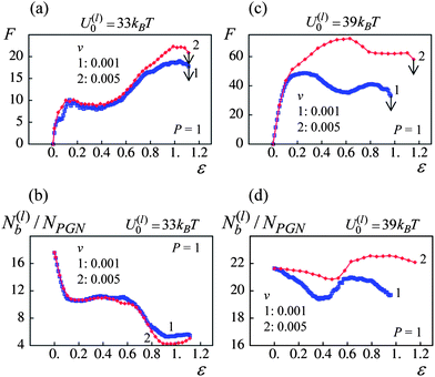 | ||
| Fig. 12 Effect of pulling velocity, v, at P = 1 on network response (blue and red lines denote pulling velocities v = 0.001 and 0.005 respectively): (a) force(F)–strain(ε) curves for U(l)0/kBT = 33. (b) Number of labile bonds/particle, N(l)b/NPGN, as a function of strain, ε, for U(l)0/kBT = 33. (c) Force(F)–strain(ε) curves for U(l)0/kBT = 39. (d) Number of labile bonds/particle, N(l)b/NPGN, as a function of strain, ε, for U(l)0/kBT = 39. | ||
In contrast, the material encompassing the stronger labile bonds exhibits ∼70% increase in W at the higher strain rate even when no permanent bonds are present (P = 0), and the enhancement of toughness is about 80% at P = 1 (Fig. 11d). It is seen in Fig. 12c that both the yield force and strain increase with an increase in the pulling velocity. The latter takes place because of the delayed rupture of the bonds as shown in Fig. 10b and the increase in the number of the stronger labile bonds (U(l)0 = 39kBT) in the system, as evident in Fig. 12d. As a result, a greater work is necessary to break the sample, i.e., the toughness increases.
IV. Conclusions
To facilitate the design of high-strength, tough networks composed of cross-linked polymer grafted nanoparticles (PGNs), we formulated a hybrid model that integrates the hierarchy of structural features and temporal events that characterize the behavior of the system. It has been previously reported that graft density and length of grafted polymer chains affect mechanical properties of bulk nanoparticles with grafted polymers.10 Researchers have also prepared several materials with degeneratively exchanging weak bonds that exhibit self-healing properties.37,39–43 Thus, our ultimate goal is to incorporate the exchanging units into hybrid polymer–nanoparticle materials and the model presented here can facilitate the fabrication of such materials.Our model combines information on the features of each PGN and the pair interaction between PGNs with the kinetics of rupturing/forming individual bonds and mechanical deformation of the entire sample. Using this model, we focused on systems of dual cross-linked PGNs, which are interconnected by both strong “permanent” bonds and weaker labile bonds, and determined the response of the material to a tensile deformation. To establish the critical parameters controlling the mechanical behavior of these materials, we varied the fraction of permanent bonds, P, the bond energies of the labile bonds, U(l)0, the thickness of the corona on the nanoparticles, q, and the strain rate.
We found that the fraction of permanent bonds plays a critical role primarily in the material encompassing the weaker labile bonds, U(l)0 = 33kBT. In these materials, increases in P lead to significant improvements in the ductility and the toughness of the dual cross-linked network. In the material with the stronger labile bonds of U(l)0 = 39kBT, increases in P lead primarily to increases in the toughness. Even at P = 0, however, the network involving the stronger labile bonds yielded a ductile, tough material. Notably, at P = 1, the toughness of the sample with the stronger labile bonds was three times greater than that of the sample with the weaker labile bonds. Furthermore, within a network connected by a P = 1 skeleton of permanent bonds, the mode of failure depended on the nature of the labile bonds. While the networks with the weaker labile bonds failed by tearing in a direction perpendicular to the deformation, the network with the U(l)0 = 39kBT bonds failed through the growth of cavities within the sample. These findings elucidate the role that the energies of the labile bonds play in the performance of the cross-linked network.
It is noteworthy that at P = 1 in both materials, the strain at break was controlled primarily by the permanent bonds. Namely, for the both types of samples, it is ultimately the permanent bonds that bear the force from the deformation and ultimately, it is their rupture that determines the value of εb.
We examined the effect of modifying the characteristics of the coated particles by increasing the corona thickness (the contour length of the grafted chain) from q = 0.75 to 1.25. This increase in q lead to an increase in the toughness, W, of both the U(l)0 = 33kBT and U(l)0 = 39kBT networks. The underlying mechanisms for the increase in toughness were, however, found to be different in these two types of materials. While the increase in toughness was due to an increase in ductility for the U(l)0 = 33kBT network, the increase in W was due to enhanced bond formation and decreased bond rupture in the network with the U(l)0 = 39kBT bonds.
From the studies on the effect of strain rate, we found that faster strain rates yield enhanced toughness due to the delayed rupture of the bonds. Namely, in these cases, the strain rate was faster than the inherent rate of bond rupture in the system and thus, the strain did not contribute to significant bond breakage. This effect was found to be pronounced for the networks encompassing the U(l)0 = 39kBT bonds and larger fraction of permanent bonds.
The above results indicate that the mechanical response of a dual cross-linked network can be controlled through modifying the bond energies of the labile bonds, the fraction of permanent bonds in the network and the structure of the polymer grafted particles. To summarize, we have shown that in a network with weaker labile bonds, an increase in fraction of permanent bonds and the contour length of the chain can yield a tough network that behaves like a polymeric material, which exhibits cold drawing/necking. On the other hand, similar changes to the network with stronger labile bonds lead to an increase in toughness, with the network characteristics being similar to that of a purely ductile material. Notably, increases in the ratio between the strain rate and the bond rupture rate can also be used to alter the response of the networks. The model developed herein provides a powerful approach for predicting how the different parameters affect the performance of such dual cross-linked materials and can be used to probe how other critical features of the system contribute to the mechanical behavior of the samples. The behavior of quasi-2D systems similar to those considered here could be studied experimentally using atomic force microscopy17,37 and mechanical testing of Langmuir films.38
In future studies, we will determine how these samples behave as they are allowed to recover from the tensile deformation i.e., as the applied force is released at different degrees of strain. Insight provided from these studies can reveal factors that contribute to strain recovery and further facilitate the design of advanced nanocomposites.
Acknowledgements
ACB and K.M. gratefully acknowledge funding from the DOE for partial support of B.V.S.I. and I.G.S. ACB also gratefully acknowledges funding from the ARO for partial support of V.V.Y.References
- S. M. Gravano and T. E. Patten, in Macromolecular Engineering. Precise Synthesis, Materials Properties, Applications, ed. K. Matyjaszewski, Y. Gnanou and L. Leibler, Wiley–VCH, Weinheim, Germany, 2007, vol. 2, ch. 28 Search PubMed.
- L. Bombalski, K. Min, H. Dong, C. Tang and K. Matyjaszewski, Macromolecules, 2007, 40, 7429–7432 CrossRef CAS.
- H. Dong, M. Zhu, J. A. Yoon, H. Gao, R. Jin and K. Matyjaszewski, J. Am. Chem. Soc., 2008, 130, 12852–12853 CrossRef CAS.
- K. Matyjaszewski and N. V. Tsarevsky, Nat. Chem., 2009, 1, 276–288 CrossRef CAS.
- H. S. Kim, C. H. Lee, P. K. Sudeep, T. Emrick and A. J. Crosby, Adv. Mater., 2010, 22, 4600–4604 CrossRef CAS.
- K. E. Mueggenburg, X. M. Lin, R. H. Goldsmith and H. M. Jaeger, Nat. Mater., 2007, 6, 656–660 CrossRef CAS.
- P. Akcora, H. Liu, S. K. Kumar, J. Moll, Y. Li, B. C. Benicewicz, L. S. Schadler, D. Acehan, A. Z. Panagiotopoulos, V. Pryamitsyn, V. Ganesan, J. Ilavsky, P. Thiyagarajan, R. H. Colby and J. F. Douglas, Nat. Mater., 2009, 8, 354–359 CrossRef CAS.
- M. McEwan and D. Green, Soft Matter, 2009, 5, 1705–1716 RSC.
- P. Voudouris, J. Choi, N. Gomopoulos, R. Sainidou, H. Dong, K. Matyjaszewski, M. R. Bockstaller and G. Fytas, ACS Nano, 2011, 5(7), 5746–5754 CrossRef CAS.
- J. Choi, C. M. Hui, J. Pietrasik, H. Dong, K. Matyjaszewski and M. R. Bockstaller, Soft Matter, 2012, 8, 4072–4082 RSC.
- A. van den Noort and W. J. Briels, Macromol. Theory Simul., 2007, 16, 742–754 CrossRef CAS.
- S. Goyal and F. A. Escobedo, J. Chem. Phys., 2011, 135, 184902 CrossRef.
- B. B. Hong and A. Z. Panagiotopoulos, J. Phys. Chem. B, 2012, 116(8), 2385–2395 CrossRef CAS.
- J. P. Gong, Y. Katsuyama, T. Kurokawa and Y. Osada, Adv. Mater., 2003, 15(14), 1155–1158 CrossRef CAS.
- G. V. Kolmakov, K. Matyjaszewski and A. C. Balazs, ACS Nano, 2009, 3(4), 885–892 CrossRef CAS.
- I. G. Salib, G. V. Kolmakov, C. N. Gnegy, K. Matyjaszewski and A. C. Balazs, Langmuir, 2011, 27(7), 3991–4003 CrossRef CAS.
- S. F. Duki, G. V. Kolmakov, V. V. Yashin, T. Kowalewski, K. Matyjaszewski and A. C. Balazs, J. Chem. Phys., 2011, 134, 084901 CrossRef.
- C. Jung Wu, A. K. Gaharwar, B. K. Chan and G. Schmidt, Macromolecules, 2011, 44(20), 8215–8224 CrossRef.
- Q. Wang, R. Hou, Y. Cheng and J. Fu, Soft Matter, 2012, 8, 6048–6056 RSC.
- J. Yang, F. Shi, C. Gong and X. Xie, J. Colloid Interface Sci., 2012, 381(1), 107–115 CrossRef CAS.
- C. N. Likos, H. Löwen, M. Watzlawek, B. Abbas, O. Jucknischke, J. Allgaier and D. Richter, Phys. Rev. Lett., 1998, 80, 4450–4453 CrossRef CAS.
- A. Jusufi, M. Watzlawek and H. Löwen, Macromolecules, 1999, 32, 4470–4473 CrossRef CAS.
- M. Daoud and J. P. Cotton, J. Phys., 1982, 43, 531–538 CAS.
- F. Lo Verso, C. N. Likos and L. Reatto, Prog. Colloid Polym. Sci., 2006, 133, 78–87 CrossRef CAS.
- A. V. Dobrynin and Y. J. Carrillo, Macromolecules, 2011, 44, 140–146 CrossRef CAS.
- G. I. Bell, Science, 1978, 200, 618–627 CAS.
- G. I. Bell, M. Dembo and P. Bongrad, Biophys. J., 1984, 45, 1051–1064 CrossRef CAS.
- S. K. Bhatia, M. R. King and D. A. Hammer, Biophys. J., 2003, 84, 2671–2690 CrossRef CAS.
- G. Diezemann and A. Janshoff, J. Chem. Phys., 2008, 129, 084904 CrossRef.
- C. M. Wijmans and E. B. Zhulina, Macromolecules, 1993, 26, 7214–7224 CrossRef CAS.
- D. Dukes, Y. Li, S. Lewis, B. Benicewicz, L. Schandler and S. K. Kumar, Macromolecules, 2010, 43, 1564–1570 CrossRef CAS.
- K. Ohno, T. Morinaga, S. Takeno, Y. Tsujii and T. Fakula, Macromolecules, 2007, 40, 9143–9150 CrossRef CAS.
- A. P. Wiita, S. R. K. Ainavarapu, H. H. Huang and J. M. Fernandez, Proc. Natl. Acad. Sci. U. S. A., 2006, 103, 7222–7227 CrossRef CAS.
- A. J. Kinloch and R. J. Young, Fracture Behaviour of Polymers, Applied Science Publishers, London, 1983 Search PubMed.
- I. M. Ward and J. Sweeney, An Introduction to the Mechanical Properties Of Solid Polymers, Wiley, Chichester, 2004 Search PubMed.
- B. R. Lawn, Fracture of Brittle Solids, Cambridge University Press, New York, 2nd edn, 1993 Search PubMed.
- J. A. Yoon, J. Kamada, K. Koynov, J. Mohin, R. Nicolay, Y. Z. Zhang, A. C. Balazs, T. Kowalewski and K. Matyjaszewski, Macromolecules, 2012, 45, 142–149 CrossRef CAS.
- J. Y. Kim, S. Raja and F. Stellacci, Small, 2011, 7, 2526–2532 CAS.
- R. Nicolay, J. Kamada, A. Van Wassen and K. Matyjaszewski, Macromolecules, 2010, 43, 4355–4361 CrossRef CAS.
- Y. Amamoto, J. Kamada, H. Otsuka, A. Takahara and K. Matyjaszewski, Angew. Chem., Int. Ed., 2011, 50, 1660–1663 CrossRef CAS.
- J. Kamada, K. Koynov, C. Corten, A. Juhari, J. A. Yoon, M. W. Urban, A. C. Balazs and K. Matyjaszewski, Macromolecules, 2010, 43, 4133–4139 CrossRef CAS.
- Y. Amamoto, H. Otsuka, A. Takahara and K. Matyjaszewski, Adv. Mater., 2012, 24, 3975–3980 CrossRef CAS.
- Y. Amamoto, H. Otsuka, A. Takahara and K. Matyjaszewski, ACS Macro Lett., 2012, 1, 478–481 CrossRef CAS.
| This journal is © The Royal Society of Chemistry 2013 |
