Prediction of active sites of enzymes by maximum relevance minimum redundancy (mRMR) feature selection†
Yu-Fei
Gao‡
a,
Bi-Qing
Li‡
b,
Yu-Dong
Cai‡
c,
Kai-Yan
Feng
d,
Zhan-Dong
Li
e and
Yang
Jiang
*a
aDepartment of Surgery, China-Japan Union Hospital of Jilin University, Changchun, People's Republic of China. E-mail: jy7555@163.com
bKey Laboratory of Systems Biology, Shanghai Institutes for Biological Sciences, Chinese Academy of Sciences, Shanghai, People's Republic of China
cInstitute of Systems Biology, Shanghai University, Shanghai, People's Republic of China
dBeijing Genomics Institute, Shenzhen Beishan Industrial Zone, Beishan Road, Yantian District, Shenzhen, People's Republic of China
eCollege of Biology and Food Engineering, Jilin Teachers' Institute of Engineering and Technology, Changchun, People's Republic of China
First published on 15th October 2012
Abstract
Identification of catalytic residues plays a key role in understanding how enzymes work. Although numerous computational methods have been developed to predict catalytic residues and active sites, the prediction accuracy remains relatively low with high false positives. In this work, we developed a novel predictor based on the Random Forest algorithm (RF) aided by the maximum relevance minimum redundancy (mRMR) method and incremental feature selection (IFS). We incorporated features of physicochemical/biochemical properties, sequence conservation, residual disorder, secondary structure and solvent accessibility to predict active sites of enzymes and achieved an overall accuracy of 0.885687 and MCC of 0.689226 on an independent test dataset. Feature analysis showed that every category of the features except disorder contributed to the identification of active sites. It was also shown via the site-specific feature analysis that the features derived from the active site itself contributed most to the active site determination. Our prediction method may become a useful tool for identifying the active sites and the key features identified by the paper may provide valuable insights into the mechanism of catalysis.
Introduction
Enzymes play pivotal roles in biological reactions, which control the flow of metabolites within a cell and catalyze almost all of the reactions that produce and modify the molecules required in a biological pathway. Only a small number of residues of an enzyme are directly involved in catalysis and the structure and chemical properties of these residues (called active sites) determine, to a certain extent, the chemical properties of the enzyme. For this reason active site residues are highly conserved during evolution. A range of approaches have been proposed to predict active sites in enzyme sequences computationally. These can be divided into two main categories: similarity transfer based methods and ab initio methods. Similarity transfer based methods first utilize tools such as BLAST, hidden Markov models (HMMs), structural templates and pattern matching to identify sequences which are homologous to those with known active site residues, and then transfer the active site residues from the characterized sequences to the uncharacterized sequences. The Catalytic Site Atlas (CSA)1 is a database that compiles active site residues of proteins with known structures from the literature. It also provides active site residue predictions, based on PSI-BLAST hits, for proteins with unknown structures, which is one of the important resources for inferring catalytic sites. The ab initio methods predict catalytic sites by exploiting the general properties of active sites, such as geometry data,2,3 the electrostatic charge of residues,4 residue buffer capacity5 and sequence conservation.6,7 These methods are highly useful when the sequences of the active sites in question are vastly different from any known active sites or they are not conserved during evolution.Some other approaches have also been used to predict active sites. Evolutionary trace (ET) is one of them which first identifies the most conserved residues in a query sequence, then maps them on the structure of the protein and finally identifies the clusters of residues which correspond to active sites.8 ET has been widely applied and succeeded in predicting active sites in 60–80% of test cases.9,10 Some motif-based methods were also used to predict functional sites, but unfortunately they usually suffered from high false positive rates.11 In terms of machine learning algorithms, neural networks12 and support vector machines13 were found in the literature to predict active site residues.
In this study, a new ab initio method was developed to predict active sites. We incorporated features of amino acid factors, sequence conservation, residual disorder feature, secondary structure and solvent accessibility. The Random Forest algorithm (RF) with the maximum relevance minimum redundancy (mRMR) method followed by incremental feature selection (IFS) was adopted as the prediction model. Ten-fold cross validation was used to evaluate the performance of our classifier. From a total of 651 features, 37 features were selected and regarded as the optimal feature set, achieving an overall prediction accuracy of 0.885687 and MCC of 0.689226 on an independent test dataset. Feature analysis showed that the features of an active site itself contributed most to the active site determination.
Materials and methods
Dataset
All active site information was retrieved from the Catalytic Site Atlas (CSA) (version 2.2.12).1 The protein sequences containing these active sites were downloaded from the PDB database.14 We removed the homology proteins in the original dataset with a threshold of 40% identified by CD-HIT15 and 1740 protein chains containing 5369 active sites were obtained. We randomly selected 1392 chains as the training dataset and the remaining 348 chains as the testing dataset. For each active site, we extracted a peptide segment with 21 residues in it centered on the active site itself, 10 residues upstream and 10 residues downstream of the active site. Peptide segments with length less than 21 were complemented by character “X”. For the training dataset, there are a total of 4328 positive samples and we randomly selected 12![[thin space (1/6-em)]](https://www.rsc.org/images/entities/char_2009.gif) 984 non-active sites as negative samples. The testing dataset includes 1041 positive samples and 3123 randomly selected negative samples.
984 non-active sites as negative samples. The testing dataset includes 1041 positive samples and 3123 randomly selected negative samples.
Feature construction
Both relevance and redundancy were quantified by mutual information (MI), which estimates how much one vector is related to another. The MI equation was defined as below:
 | (1) |
Let Ω denote the whole feature set, Ωs denote the already-selected feature set containing m features and Ωt denote the to-be-selected feature set containing n features. The relevance D between a feature f in Ωt and the target c can be calculated by:
| D = I(f,c) | (2) |
The redundancy R between a feature f in Ωt and all the features in Ωs can be calculated by:
 | (3) |
To get the feature fj in Ωt with maximum relevance and minimum redundancy, the mRMR function combines eqn (2) and (3) and is defined as below:
 | (4) |
The mRMR feature rating would be executed N rounds when given a feature set with N (N = m + n) features. After N rounds of execution, a feature set S is produced:
 | (5) |
In S, index h indicates at which round the feature is selected. The smaller the index h is, the earlier the feature satisfies eqn (4) and the better the feature is.
1. Suppose that the number of training cases is N. Take N cases at random – but with replacement from the original data. These samples compose the training set for growing the tree, while the remaining are used to evaluate the performance of the decision tree.
2. If there are M input variables, choose a number m that is much less than M. At each node, m variables are selected randomly out of the M variables and the most optimized split on these m variables is employed to split the node.
3. Each tree is fully grown and not pruned.
To classify a new query sample coded by an input vector, put it into each of the trees in the forest. Each decision tree provides a predicted class. The class with the most votes will be output as the predicted class of the random forest.
In Weka 3.6.4,33 the classifier named Random Forest implements the random forest predictor described above. In this study, it was employed to make a prediction. Notably, it was run with default parameters. In detail, Random Forest consists of 10 decision trees and the parameter m in step 2 is set to [log2M + 1].
Weka (Waikato Environment for Knowledge Analysis),33 developed by University of Waikato in New Zealand, is a free software integrating several state-of-the-art machine learning algorithms and data analysis tools. It can be downloaded from the website http://www.cs.waikato.ac.nz/ml/weka/. Since the user of the Weka can try different kinds of algorithms, compare their performance, and select a suitable algorithm for generating an effective predictive model, it is widely used by many investigators to analyze and predict various data about different biological problems.34–42
 | (6) |
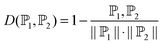
![[Doublestruck P]](https://www.rsc.org/images/entities/char_e173.gif) 1 and 2 are two vectors representing two samples, 1·2 is their dot product, ∥1∥ and ∥2∥ are their moduli. The smaller the D(1, 2), the more similar the two samples are.
1 and 2 are two vectors representing two samples, 1·2 is their dot product, ∥1∥ and ∥2∥ are their moduli. The smaller the D(1, 2), the more similar the two samples are.
For an intuitive illustration of how NNA works, see Fig. 5 of ref. 52.
 | (7) |
During the IFS procedure, features in the ranked feature set are added one by one from higher to lower rank. A new feature set is composed when one feature is added. Thus N feature sets would be composed, given N ranked features. The ith feature set is:
| Si = {f1, f2,…, fi}(1 ≤ i ≤ N) | (8) |
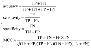
For each of the N feature sets, an RF predictor was constructed and tested using a ten-fold cross-validation test. With N prediction accuracies, sensitivities, specificities and MCCs calculated, we obtain an IFS table with one column being the index i and the other columns the prediction accuracy, sensitivity, specificity and MCC. The optimal feature set (Soptimal) is the one, using which the predictor achieves the best prediction performance.
Results and discussion
The mRMR result
After running the mRMR software, we obtained two tables (ESI†, S1): one is called the MaxRel feature table that ranks the 179 reduced features according to their relevance to the class of samples; and the other is called the mRMR feature table that lists the ranked 179 reduced features with the mRMR criteria. In the mRMR feature table, a feature with a smaller index implies that it is a more important one for active site prediction. Such list of ranked features is used in the following IFS procedure for the optimal feature set selection.IFS and incremental analysis result
By adding the ranked features one by one, we built 179 individual predictors for the 179 sub-feature sets to predict the active sites. We then tested the prediction performance for each of the 179 predictors and obtained the IFS results (ESI†, S2). Shown in Fig. 1 is the IFS curve plotted based on the data of ESI†, S2. As we can see from the figure, the MCC reached its first peak at 0.698309 when 37 features given in ESI†, S3, were used. Then the MCC fluctuated with the increase of features, and reached the maximum value of 0.701644 with 199 features. Nevertheless, it only promoted the MCC by 0.003335, compared with increase of 162 features. To avoid introduction of irrelevant features, we regarded the 37 features as the optimal feature set for the classifier. Based on these 37 features, the prediction sensitivity, specificity and accuracy were 0.742606, 0.938155, and 0.889268, respectively (Table 1).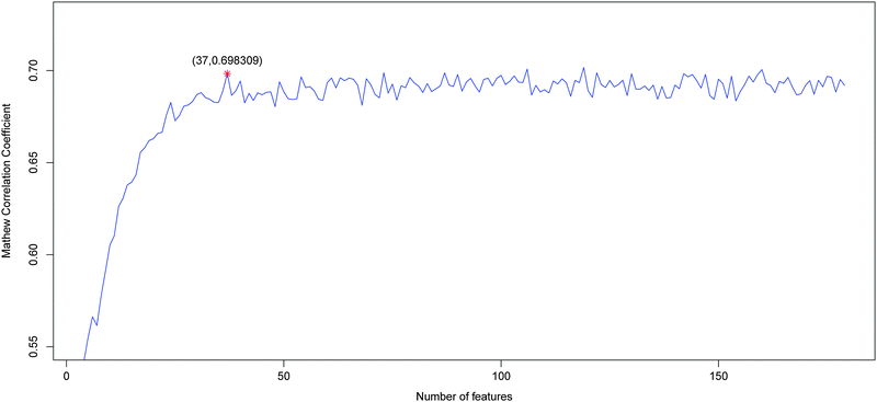 | ||
| Fig. 1 Plot showing the values of MCC against different number of features based on the data in ESI†, S2. When 37 features were used, the first peak of MCC was obtained. These 37 features were considered as the optimal feature set for our classifier. | ||
| Dataset | Method | ![[Fraktur R]](https://www.rsc.org/images/entities/char_e18f.gif) sena sena |
speb |
spec |
MCCd |
|---|---|---|---|---|---|
| a Sensitivity. b Specificity. c Accuracy. d Matthews's correlation coefficient. | |||||
| Training dataset | Our | 0.742606 | 0.938155 | 0.889268 | 0.698309 |
| SVM | 0.711183 | 0.942853 | 0.884935 | 0.682935 | |
| NNA | 0.777957 | 0.891097 | 0.862812 | 0.647973 | |
| Testing dataset | Our | 0.739673 | 0.934358 | 0.885687 | 0.689226 |
| SVM | 0.723343 | 0.93692 | 0.883525 | 0.681308 | |
| NNA | 0.787704 | 0.893692 | 0.867195 | 0.659565 | |
Analysis of the optimal feature set
The distribution of the number of each type of features in the final optimal feature set was investigated and shown in Fig. 2A. As we can see from the figure, of the 37 optimal features, 20 belong to the PSSM conservation score, 1 to the amino acid factor, 6 to the secondary structure, 10 to the solvent accessibility, and no disorder, suggesting that except disorder all other four types of features contribute to the prediction of active sites. The site-specific distribution of the optimal feature set (Fig. 2B) revealed that site 11 played the most important role in the determination of active sites, which indicated that the features derived from the active site itself contributed more to the prediction of active sites than those of flanking residues.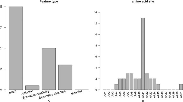 | ||
| Fig. 2 Bar plots showing (A) the feature distribution for the 37 optimal features, and (B) the corresponding site distribution. It can be seen from panel A that of the 37 optimal features, 20 belong to the PSSM conservation score, 1 to the amino acid factor, 6 to the secondary structure, 10 to the solvent accessibility, and none to the disorder. It can be seen from panel B that site 11 played the most important role in the determination of active site. | ||
Feature analysis of PSSM conservation score
As mentioned above, there were 20 PSSM conservation features, which account for the greatest proportion of the optimal 37 features. We investigated the number of each kind of amino acids of the PSSM features (Fig. 3A) and found that conservations against mutations to the 20 amino acids impact the active site prediction differently. Mutations to amino acid lysine (K) influence the active site determination the most and mutations to amino acid glutamic acid (E) and threonine (T) also influence more than others. It has been reported that E and K were highly conserved among active residues.3 The first feature in the mRMR feature list (ESI†, S3) is the PSSM feature at site 11 against transition to amino acid valine (V), indicating that this is the most important feature for determining active sites. In addition, the features within the top 10 features in the final optimal feature list contain two other PSSM conservation features: the conservation status against residue alanine (A) at site 11 (index 3, “AA11_pssm_1”) and the conservation status against residue threonine (T) at site 11 (index 9, “AA11_pssm_17”). It implied that the conservation status of the active site itself was the most important feature for the prediction of the active site which was consistent with the fact that active site residues are highly conserved.55 We also investigated the number of PSSM features at each site (Fig. 3B) and found that the conservation status of site 11 played the most important role in the prediction of active sites, as shown in Fig. 3B.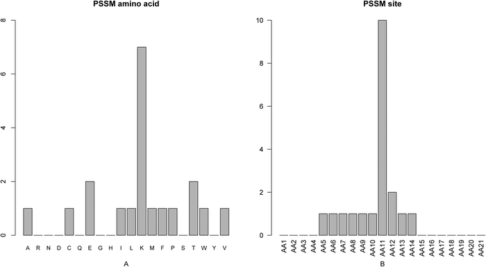 | ||
| Fig. 3 Bar plots showing the distribution in the final optimal feature set for (A) the PSSM score, and (B) the corresponding specific site score. It can be seen from panel A that the conservation against mutations to amino acid lysine (K) impacts most the active site determination and mutations to amino acid glutamic acid (E) and threonine (T) also impact relatively more than others. It can be seen from panel B that the conservation status of site 11 played the most important role in the prediction of active sites. | ||
Analysis of the amino acid factor
The number of each type of amino acid factor (Fig. 4A) and the number of the amino acid factor at each site (Fig. 4B) were analyzed. It was found that codon diversity was the most important feature. It has been shown that proteases with P225 typically use a TCN codon for S195, whereas proteases with Y225 use an AGY codon.56,57 In addition, there is no clear selective codon usage within all lipases or all esterases, though codon usage seems to be well conserved within closely related sequences.58 Therefore, the codon diversity may be important for the determination of the active site. According to Fig. 4B, residues at site 11 contribute most to active site prediction. The codon diversity of site 11 has an index of 6 in the final optimal feature list, indicating that it is one of the most important features for active site prediction.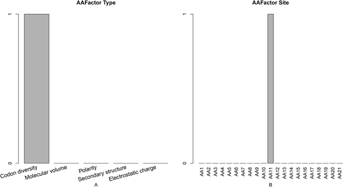 | ||
| Fig. 4 Bar plots showing the distribution in the final optimal feature set for (A) the features of amino acid factor, and (B) the corresponding specific site score. It can be seen from panel A that codon diversity was the most important feature. It can be seen from panel B that residues at site 11 contribute the most to active site prediction. | ||
Analysis of disorder feature
Among the optimal features, none of 21 disorder features were selected, which suggested that the disorder feature may not be important for active site prediction.Feature analysis of solvent accessibility
We investigated the 10 features of solvent accessibility in the optimal feature set (Fig. 5). As shown in Fig. 5A, there were more features of exposed solvent accessibility than buried ones, indicating that active sites were skewed toward larger accessible surface areas, as it was reported in ref. 13 that relative positions on protein surface were the most important ones of active sites. It has been shown that activation of the enzyme involves the displacement of the lid to expose the active site.59 In addition, it has been reported that large conformational changes are required to trigger the exposure of the active site of the enzyme.60 As shown in Fig. 5B, the solvent accessibility at site 11 exerts more influence on active site determination.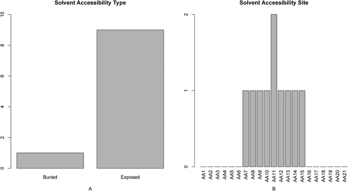 | ||
| Fig. 5 Bar plots showing the distribution in the final optimal feature set for (A) the solvent accessibility score, and (B) the corresponding specific site score. It can be seen from panel A that the score of the solvent accessibility with exposed characteristics was greater than the buried, indicating that features of exposed solvent accessibility are more important for active site determination. It can be seen from panel B that the features of solvent accessibility at site 11 impact the active site determination relatively more. | ||
Feature analysis of secondary structure
The feature and site-specific distribution of the secondary structure in the optimal feature set was shown in Fig. 6. From panel A of the figure we can see that features of helix and strand contribute to the active site determination; from panel B we can see that features of secondary structure at sites 4–8 and site 21 exert more influence on the active site determination.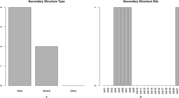 | ||
| Fig. 6 Bar plots showing the distribution in the final optimal feature set for (A) the secondary structure score, and (B) the corresponding specific site score. It can be seen from panel A that the secondary structures of helix and strand affect active site determination. It can be seen from panel B that the features of secondary structure at sites 4–8 and site 21 impact the active site determination relatively more. | ||
Comparing performance of different methods
To assess the performance of our predictor, we compared it with other two widely used machine learning approaches including SVM and NNA based on the same training and independent testing datasets. The prediction accuracies for positive, negative and total samples are shown in Table 1. From Table 1, we can see that though the specificity of the SVM method (0.942853) for the training dataset is a litter better than ours (0.938155), the overall prediction accuracy (0.884935) and MCC (0.682935) are not as good as ours (Ac: 0.889268, MCC: 0.698309). The sensitivity of the NNA method (0.777957) for the training dataset is better than ours (0.742606), but the overall accuracy (0.862812) and MCC (0.647973) are worse than ours (Ac:0.889268, MCC:0.698309). For the testing dataset, the result is similar to the training dataset (Table 1). Therefore, our method has the best performance among these three methods. The sensitivity, specificity, accuracy and MCC of SVM and NNA for the training dataset are listed in ESI†, S4.Directions for experimental validation
It is worthwhile pointing out that the important features at some specific sites may provide useful clues for finding and validating new determinants of protein active sites by experiments. For example, it was found in this study that mutations to amino acids K, E and T had relatively more impact on the prediction performance, which was consistent with the finding that K and E were highly conserved residues in active residues.3 It was revealed that the codon diversity is an important feature for determination of active site, which is in agreement with previous studies.56–58 We found in our study that the number of solvent accessibility features with exposed characteristics was greater than that of the buried, consistent with some reports stating that active sites were skewed toward larger surface accessible areas.13,59,60 Therefore, it is worthwhile investigating the remaining features in the optimal feature set by experimental validation.Conclusion
In this study, we developed a new method for predicting and analyzing protein active sites. Our method incorporated features of not only sequence conservation, but also physicochemical properties, solvent accessibility, secondary structure and residue disorder status of active sites. By means of feature selection, 37 optimal features were selected, which were regarded as the most contributing features to the prediction of active sites. Based on these features, our approach achieved an overall accuracy of 0.885687 and MCC of 0.689226 on an independent test dataset and outperformed other two widely used machine learning approaches. The optimal features may shed some light on the mechanism of catalysis, and provide guidelines for experimental validations. The software is available upon request.Acknowledgements
This contribution is supported by National Basic Research Program of China (2011CB510102, 2011CB510101), Innovation Program of Shanghai Municipal Education Commission (No.12YZ120, No. 12ZZ087), Natural science fund projects of Jilin province (201215059), development of science and technology plan projects of Jilin province (20100733, 201101074), SRF for ROCS, SEM (2009-36), Scientific Research Foundation (Jilin Department of Science & Technology, 200705314, 20090175, 20100733), Scientific Research Foundation (Jilin Department of Health, 2010Z068), SRF for ROCS (Jilin Department of Human Resource & Social Security, 2012-2014).References
- C. T. Porter, G. J. Bartlett and J. M. Thornton, Nucleic Acids Res., 2004, 32, D129–D133 CrossRef CAS.
- R. Greaves and J. Warwicker, J. Mol. Biol., 2005, 349, 547–557 CrossRef CAS.
- M. Ota, K. Kinoshita and K. Nishikawa, J. Mol. Biol., 2003, 327, 1053–1064 CrossRef CAS.
- A. H. Elcock, J. Mol. Biol., 2001, 312, 885–896 CrossRef CAS.
- M. J. Ondrechen, J. G. Clifton and D. Ringe, Proc. Natl. Acad. Sci. U. S. A., 2001, 98, 12473–12478 CrossRef CAS.
- K. M. Mayer, S. R. McCorkle and J. Shanklin, BMC Bioinf., 2005, 6, 284 CrossRef.
- A. R. Panchenko, F. Kondrashov and S. Bryant, Protein Sci., 2004, 13, 884–892 CrossRef CAS.
- O. Lichtarge, H. R. Bourne and F. E. Cohen, J. Mol. Biol., 1996, 257, 342–358 CrossRef CAS.
- H. Yao, D. M. Kristensen, I. Mihalek, M. E. Sowa, C. Shaw, M. Kimmel, L. Kavraki and O. Lichtarge, J. Mol. Biol., 2003, 326, 255–261 CrossRef CAS.
- H. Yao, I. Mihalek and O. Lichtarge, Proteins, 2006, 65, 111–123 CrossRef CAS.
- A. H. Liu, X. Zhang, G. A. Stolovitzky, A. Califano and S. J. Firestein, Genomics, 2003, 81, 443–456 CrossRef CAS.
- A. Gutteridge, G. J. Bartlett and J. M. Thornton, J. Mol. Biol., 2003, 330, 719–734 CrossRef CAS.
- N. V. Petrova and C. H. Wu, BMC Bioinf., 2006, 7, 312 CrossRef.
- H. M. Berman, J. Westbrook, Z. Feng, G. Gilliland, T. N. Bhat, H. Weissig, I. N. Shindyalov and P. E. Bourne, Nucleic Acids Res., 2000, 28, 235–242 CrossRef CAS.
- W. Li and A. Godzik, Bioinformatics, 2006, 22, 1658–1659 CrossRef CAS.
- S. F. Altschul, T. L. Madden, A. A. Schaffer, J. Zhang, Z. Zhang, W. Miller and D. J. Lipman, Nucleic Acids Res., 1997, 25, 3389–3402 CrossRef CAS.
- P. E. Wright and H. J. Dyson, J. Mol. Biol., 1999, 293, 321–331 CrossRef CAS.
- A. K. Dunker, C. J. Brown, J. D. Lawson, L. M. Iakoucheva and Z. Obradovic, Biochemistry, 2002, 41, 6573–6582 CrossRef CAS.
- J. Liu, H. Tan and B. Rost, J. Mol. Biol., 2002, 322, 53–64 CrossRef CAS.
- P. Tompa, Trends Biochem. Sci., 2002, 27, 527–533 CrossRef CAS.
- K. Peng, P. Radivojac, S. Vucetic, A. K. Dunker and Z. Obradovic, BMC Bioinf., 2006, 7, 208 CrossRef.
- S. Kawashima and M. Kanehisa, Nucleic Acids Res., 2000, 28, 374 CrossRef CAS.
- W. R. Atchley, J. Zhao, A. D. Fernandes and T. Druke, Proc. Natl. Acad. Sci. U. S. A., 2005, 102, 6395–6400 CrossRef CAS.
- J. Cheng, A. Z. Randall, M. J. Sweredoski and P. Baldi, Nucleic Acids Res., 2005, 33, W72–W76 CrossRef CAS.
- H. Cramér, Mathematical Methods of Statistics, Princeton University Press, Princeton, 1946 Search PubMed.
- M. Kendall and A. Stuart, The advanced theory of statistics: vol.2 – inference and relationship, Macmillan, New York, 1979 Search PubMed.
- K. M. Harrison, T. Kajese, H. I. Hall and R. Song, Public Health Rep., 2008, 123, 618–627 Search PubMed.
- H. Peng, F. Long and C. Ding, IEEE Trans. Pattern Anal. Mach. Intell., 2005, 27, 1226–1238 CrossRef.
- N. Zhang, B.-Q. Li, S. Gao, J.-S. Ruan and Y.-D. Cai, Mol. BioSyst., 2012, 8, 2946–2955 RSC.
- B.-Q. Li, L.-L. Hu, L. Chen, K.-Y. Feng, Y.-D. Cai and K.-C. Chou, PLoS One, 2012, 7, e39308 CAS.
- B.-Q. Li, K.-Y. Feng, L. Chen, T. Huang and Y.-D. Cai, PLoS One, 2012, 7, e43927 CAS.
- L. Breiman, Mach. Learn., 2001, 45, 5–32 CrossRef.
- I. H. Witten and E. Frank, Data Mining: Practical machine learning tools and techniques, Morgan Kaufmann Pub, 2005 Search PubMed.
- L. Chen, L. Lu, K. R. Feng, W. J. Li, J. Song, L. L. Zheng, Y. L. Yuan, Z. B. Zeng, K. Y. Feng, W. C. Lu and Y. D. Cai, J. Comput. Chem., 2009, 30, 2248–2254 CAS.
- T. Huang, L. Chen, Y. Cai and C. Chou, PLoS One, 2011, 6, e25297 CAS.
- O. Ivanciuc, Curr. Top. Med. Chem., 2008, 8, 1691–1709 CrossRef CAS.
- N. V. Petrova and C. H. Wu, BMC Bioinf., 2006, 7, 312 CrossRef.
- M. G. Ravetti and P. Moscato, PLoS One, 2008, 3, e3111 Search PubMed.
- J. C. Braisted, S. Kuntumalla, C. Vogel, E. M. Marcotte, A. R. Rodrigues, R. Wang, S. T. Huang, E. S. Ferlanti, A. I. Saeed and R. D. Fleischmann, BMC Bioinf., 2008, 9, 529 CrossRef.
- L. C. Borro, S. R. M. Oliveira, M. E. B. Yamagishi, A. L. Mancini, J. G. Jardine, I. Mazoni, E. Santos, R. H. Higa, P. R. Kuser and G. Neshich, Genet. Mol. Res., 2006, 5, 193–202 CAS.
- L. Zhang, Intell. Comput. Technol., 2012, 334–341 CrossRef.
- K. Peng, P. Radivojac, S. Vucetic, A. K. Dunker and Z. Obradovic, BMC Bioinf., 2006, 7, 208 CrossRef.
- V. N. Vapnik, Statistical Learning Theory, Wiley-Interscience, New York, 1998 Search PubMed.
- B. Yao, L. Zhang, S. Liang and C. Zhang, PLoS One, 2012, 7, e45152 CAS.
- X. Wang, G. Mi, C. Wang, Y. Zhang, J. Li, Y. Guo, X. Pu and M. Li, Comput. Biol. Med., 2012, 42, 1053–1059 CrossRef CAS.
- X. B. Wan, Y. Zhao, X. J. Fan, H. M. Cai, Y. Zhang, M. Y. Chen, J. Xu, X. Y. Wu, H. B. Li, Y. X. Zeng, M. H. Hong and Q. Liu, PLoS One, 2012, 7, e31989 CAS.
- J. H. Friedman, F. Baskett and L. J. Shustek, IEEE Trans. Inf. Theory, 1975, C–24, 1000–1006 Search PubMed.
- T. Denoeux, IEEE Trans. Syst., Man Cybern., 1995, 25, 804–813 CrossRef.
- B. Q. Li, L. L. Hu, S. Niu, Y. D. Cai and K. C. Chou, J. Proteomics, 2012, 75, 1654–1665 CrossRef CAS.
- L. L. Hu, S. B. Wan, S. Niu, X. H. Shi, H. P. Li, Y. D. Cai and K. C. Chou, Biochimie, 2011, 93, 489–496 CrossRef CAS.
- B.-Q. Li, T. Huang, L. Liu, Y.-D. Cai and K.-C. Chou, PLoS One, 2012, 7, e33393 CAS.
- K. C. Chou, J. Theor. Biol., 2011, 273, 236–247 CrossRef CAS.
- R. Kohavi, A Study of Cross-Validation and Bootstrap for Accuracy Estimation and Model Selection, San Mateo, 1995 Search PubMed.
- B.-Q. Li, Y.-D. Cai, K.-Y. Feng and G.-J. Zhao, PLoS One, 2012, 7, e45854 CAS.
- J. Mistry, A. Bateman and R. D. Finn, BMC Bioinf., 2007, 8, 298 CrossRef.
- Q. D. Dang and E. Di Cera, Proc. Natl. Acad. Sci. U. S. A., 1996, 93, 10653–10656 CrossRef CAS.
- D. M. D. Irwin, Nature, 1988, 336, 429–430 CrossRef CAS.
- M. R. e. Gewely, Biotechnology annual review, Elsevier, Amsterdam, vol. 1, 1995 Search PubMed.
- G. H. Peters, O. H. Olsen, A. Svendsen and R. C. Wade, Biophys. J., 1996, 71, 119–129 CrossRef CAS.
- J. Polaina and A. P. MacCabe, Industrial Enzymes: Structure, Function And Applications, Springer, 2007 Search PubMed.
Footnotes |
| † Electronic supplementary information (ESI) available. See DOI: 10.1039/c2mb25327e |
| ‡ These authors contributed equally. |
| This journal is © The Royal Society of Chemistry 2013 |