Introducing a standard method for experimental determination of the solvent response in laser pump, X-ray probe time-resolved wide-angle X-ray scattering experiments on systems in solution

Abstract

In time-resolved laser pump, X-ray probe wide-angle X-ray scattering experiments on systems in solution the structural response of the system is accompanied by a solvent response. The solvent response is caused by reorganization of the bulk solvent following the laser pump event, and in order to extract the structural information of the solute, the solvent response has to be treated. Methodologies capable of doing so include both theoretical modelling and experimental determination of the solvent response. In the work presented here, we have investigated how to obtain a reproducible solvent response—the solvent term—experimentally when applying laser pump, X-ray probe time-resolved wide-angle X-ray scattering. The solvent term describes difference scattering arising from the structural response of the solvent to changes in the hydrodynamic parameters: pressure, temperature and density. We present results based on NIR and dye mediated solvent heating, and demonstrate that the solvent response is independent of the heating method. The NIR heating is shown to be rendered unusable by higher order effects under certain experimental conditions, while the dye mediated solvent heating is demonstrated to exhibit first order behaviour with respect to the amount of energy deposited in the solution. We introduce a standardized method for recording solvent responses in laser pump, X-ray probe time-resolved X-ray wide-angle scattering experiments by using dye mediated solvent heating. Furthermore, we have generated a library of solvent terms, which can be used to describe the solvent term in any TRWAXS experiment, and made it available online.

---

1 Introduction

Laser pump, X-ray probe time-resolved wide-angle X-ray scattering (TRWAXS) experiments are one of the few techniques that allow for the direct study of transient structural changes of species in solution. In the earliest TRWAXS experiments, systems showing structural changes on the nanosecond timescale were investigated using synchrotron radiation.^1,2 The timescale has since been expanded to the picosecond regime,^3–9 and with the availability of the X-ray free electron lasers the femtosecond timescale has recently become accessible.^10–15 TRWAXS on systems in solution is an established technique,^16–34 which has been used to directly show structural changes occurring during photoinitiated uni- and bi-molecular chemical reactions in solution; as well as the temporal evolution of these reactions (references relating to X-ray absorption have been included for completeness).^35–46 The data obtained in a TRWAXS experiment—difference scattering images generated by subtracting an image recorded before the pump has arrived at the sample from an image recorded in a given time after the pump has arrived at the sample—arise from structural changes, which can be divided into three terms:^35,47,48

(i) structural changes of the solute (solute term),

(ii) structural changes of the bulk solvent (solvent term),

(iii) structural changes of the solvent-shell surrounding the solute (solute–solvent cross-term).

In order to obtain information on the structural changes of the solute, the other terms have to be determined before the solute term can be reliably extracted from the data. At present, the solute–solvent cross-term can only be determined experimentally when convoluted with the solute term and the solvent term, while computational chemistry can reproduce the solute–solvent cross-term independently.^26,49 The solvent term can also be evaluated theoretically, in particular by Molecular Dynamics (MD) simulations,^{27–30,33–35,48,50–53} or it can be determined experimentally.^{30–35,48,50,52} In the single study where both experimental and theoretical solvent terms have been used to extract structural information from TRWAXS data, the experimentally determined solvent terms were shown to give a more accurate description of the data.⁴⁸

Taking a step back from the context of TRWAXS, the solvent responses determined here are direct structural fingerprints of the changes in molecular structure of the solvent occurring with changes in temperature, pressure and density. As they are recorded using pseudo-monochromatic X-rays, the data we make available can be used to describe the transient scattering of a solution at any X-ray source (e.g. at free electron X-ray lasers, where experiment time is highly limited). Futhermore, they may also be used to benchmark MD-simulations. A good correlation between MD-simulations and TRWAXS data may show which structural changes correspond to the observed fingerprint. Here, we do a direct interpretation relating the fingerprint to inter-molecular distances. While the solvent term has been used extensively in data processing to obtain the solute term,^{30–35,48,50,52} a unified investigation of the solvent term for several solvents had not been performed.

The experimental determination of the solvent response relies on point heating of the solvent. We define point heating as an event where individual sites (molecules) in a solution are promoted to a high-energy state, from which they release the energy to the surrounding solvent, resulting in an overall heating of the solution (point heating is explained in detail in the ESI†). Point heating of the solvent can be achieved by three methods: direct near-infrared (NIR) heating of the solvent through exciting vibrational overtones of individual solvent molecules,^30,47,48 UV photolysis of individual solvent molecules resulting in bulk heating,^52,54 and dye mediated heating of the solvent.^31–35 Depositing hard UV radiation in the sample volume is not considered further in this work, as it leads to undesired chemical reactions.⁵⁵ We have used NIR and dye mediated solvent heating to obtain the data needed to determine the solvent term in eight different solvents. We demonstrate that the results of dye mediated and NIR heating are identical in methanol at low laser fluencies, and that dye mediated solvent heating can be achieved using a large range of dye concentrations, wavelengths and laser fluencies. We have employed dye mediated solvent heating in a series of TRWAXS experiments in order to generate a library with parameters describing the solvent term for these solvents. The library is freely accessible online,⁵⁶ and the dyes used to generate the library can be acquired by contacting the authors.⁵⁷

2 Experimental

2.1 Dye synthesis and characterization

The dyes (see Fig. 2, below) were chosen based on their spectral range and solubility. For water, a yellow dye, Fast Yellow, was chosen. Fast Yellow (1, sodium 4-aminoazobenzene-3,4′-disulphonate, CAS 2706-28-7) is commercially available with suitable purity. For the organic solvents a yellow and a red azobenzene were selected, 4-bromo-4′-(N,N-diethylamino)-azobenzene⁵⁸ (2, CAS 22700-62-5) and 4-(N,N-diethylamino)-2-methoxy-4′-nitro-azobenzene⁵⁹ (3, CAS 6373-95-1) were synthesized using an adapted method based on a large scale synthesis of methyl red from organic synthesis.⁶⁰ The purity of the dyes2 and 3 was determined by NMR, GC-MS and elementary analysis and was found to be higher than 99%.

The absorption coefficients were determined by three independent measurements, by dissolving three different weighed quantities of a sample in an appropriate volume of solvent. The error is estimated to be <10%. The solubility of the dyes was determined by making a saturated solution in each of the selected solvents, which were then left to equilibrate overnight. 50 μl of each solution was diluted to 200 ml and the absorption spectrum measured. The absorption coefficients, determined as described above, were then used to determine the solubility for each dye–solvent combination.

2.2 Experimental set-up – ESRF ID09B

Time-resolved scattering measurements were performed at the dedicated time-resolved laser pump, X-ray probe beamline ID09B at the ESRF (details of the setup are given in Appendix B).

The sample was placed in a temperature controlled water-reservoir kept at 25 °C for the pump–probe measurements. The sample was cycled in a fast-flowing liquid jet setup with a sapphire nozzle producing a 300 μm jet flowing at 2 m s⁻¹, ensuring total replenishment of the sample volume between each pump–probe event. An external temperature controller ensured that the sample temperature was kept within 0.1 °C of the reservoir temperature.

The sizes of the laser and X-ray focus were measured using a pinhole and determined to be 350 μm (h) × 340 μm (v) for the laser spot and 120 μm (h) × 80 μm (v) for the X-rays (horizontal and vertical dimensions respectively). The laser pulse length was 1.2 ps, and unless otherwise noted, the excitation energy was 200 μJ per pulse.

The pump–probe scattering images were accumulated in sequences of 2–5 images with a time delay between the laser pump and X-ray probe given by Δt = t_probe − t_pump. The sequences were spaced with a negative time delay (that is the X-rays arriving before the laser pump), which were used as references. Each image was integrated for 5 seconds, corresponding to 5000 individual pump–probe events. At each time delay 50–200 images were acquired.

Additionally, steady-state measurements were conducted for all solvents at different temperatures. The reservoir temperature was changed, and the samples were allowed to reach the equilibrium temperature before the measurement was started. The high speed chopper (see Appendix B for details) was moved slightly out of the X-ray beam increasing the opening time from 260 ns to 2 μs, letting a pulse-train of 11 X-ray pulses through at a time reducing the exposure times to ∼1 second.

2.3 X-ray data reduction

The 2D scattering patterns from the CCD detector were corrected for geometry and polarization (see ESI† for details). This was followed by azimuthal integration yielding 1D curves of the scattering intensity S(2θ) versus the scattering angle. The S(2θ) curves were scaled to the sum of the coherent and incoherent scattering of a single solvent molecule at high scattering angles. Scattering at high angles is dominated by the incoherent scattering and therefore relatively insensitive to structural changes as described elsewhere.^31,48

Difference scattering intensities ΔS(2θ) were generated from the scattering curves recorded at a positive time delay by subtracting the average of the two nearest scattering curves recorded at a negative time delay. Difference curves from the same pump–probe time-delay (Δt) were summed after an outlier rejection based on a point-by-point implementation of Chauvenet's criterion. The noise level was estimated from a second-order polynomial fit to a running 20 point interval in the data set as described previously.³⁵ The difference scattering curves presented in this work are plotted against the wave vector transfer ΔS(Q), Q = 4π/λ × sin(2θ). In order to generate these plots, the X-ray energy has been approximated by a monochromatic 18 keV spectrum.⁶¹

3 Theory

3.1 Energy dissipation from excited molecular states

The transient evolution of the energy deposited by the pump-laser in a single pump–probe cycle is described by:

The pump-laser excites the solute from its ground state (S₀), the initial electronically excited (S_n*) state relaxes via a combination of intra-molecular vibrational redistribution^62–64 (IVR) and internal conversion (IC) to a vibrationally excited state of the lowest electronically excited state (S₁*), which subsequently relaxes through vibrational relaxation (VR) to the vibrational ground state of the lowest electronically excited state (S₁); these processes occur within the first picoseconds after excitation.⁶⁵ The electronically excited state decays to a vibrationally excited electronic ground state (S₀*). The last step in the energy transfer cascade is the VR step back to the vibronic ground state of the solute (S₀).⁶⁶ Note that energy is only transferred out of the solute through vibrational relaxation.

The timescales of the processes dictate that energy will be deposited into the solvent in two separate steps. The first step deposits energy corresponding to the difference between S_n* and S₁ on a ∼1–100 ps timescale. The second energy transfer occurs on a timescale directly linked to the lifetime of the lowest electronically excited state of the solute, which can be anything from picoseconds to seconds.

Vibrational relaxation deposits vibrational energy directly as heat into the solvent shell, which then dissipates to the bulk solvent giving rise to the structural changes seen in the TRWAXS data; this is the solvent term defined in the introduction.

3.2 Energy dissipation pathways in azo-benzene

Azobenzene can exist as a cis (Z-) and trans (E-) isomer, where the latter is the most stable. The two isomers can interconvert upon irradiation, a process that has been intensely studied.^62,67–73 The trans isomer is the more stable of the two. Donor and acceptor substituents increase the energy difference between the two isomers, and decrease the barrier of inter-conversion.⁷⁴ Thus, donor–acceptor substituted azobenzenes are isolated as the pure trans form. The cis/trans isomerization is associated with a potential loss of energy that otherwise would have been deposited in the solvent, as the formation energy of the cis form is higher than for the trans form. A cautious estimate based on numbers for azobenzene gives an energy-loss of <5% for excitation by light with wavelengths lower than 500 nm if only ground state absorption is considered.

Ultrafast dynamics govern the processes occurring in azobenzene upon photo-excitation.⁷⁵ The IC from the electronically exited state to the electronic ground state is very fast (∼200 fs), and proceeds via the cis/trans isomerization process.^69–73 The time it takes for full VR to occur in azobenzene is solvent dependent and has been measured in hexane (16 ps), acetonitrile (17 ps) and DMSO-d₆ (20 ps).^62,68,76 We can conclude that at experiment times ≥100 ps no molecular signature can be present as the azo-benzene molecule will have returned to the ground state, and consequently must have transferred all absorbed energy to the solvent.

As volume changes following an isomerisation event will increase the local density, this change has to be evaluated. A combination of transient grating and photoacoustic experiments, computational methods and structural considerations have been done for azo-benzene.^77,78 The results yield values of the volume change caused by isomerisaton slightly above and below ΔV = 0 ų per molecule, and the two experimentally determined volume differences are of opposite sign. As the volume change represents less than a change of 5% of the total molecular volume we can ignore volume changes due to isomerisation in this study.

3.3 Thermodynamics of pump–probe experiments

The hydrodynamics of the pump–probe experiment has been discussed in detail by Cammarata et al.⁴⁸ A brief summary will be presented here.

The speed of a thermal redistribution after a point heating event is given by eqn (1).⁷⁹

where r is the distance from the source of the point heating, t is the time since the heating event, χ is the thermometric conductivity and κ is the thermal conductivity (eqn (2)).

The distance from the point of origin to the half maximum of the heat distribution is then given by:

The relevant material constants for all solvents included in this study are compiled in Table 1. For an excitation fraction of 30% of a 1 mM solution of a dye molecule, the average distance between centres of heat deposition is 22 nm. It follows that the FWHM of the expanding thermal distributions from neighbouring centres of heat deposition will meet after an average of ∼200 ps establishing homogeneity of the sample temperature distribution.

Table 1 Physical properties of the solvents required for the calculation of the solvent term at ambient temperature and pressure. The listed properties are from ref. 83 unless otherwise noted

Solvent	C V /J mol^−1 K^−1	C P /J mol^−1 K^−1	ρ /g cm^−3	κ /W m^−1 K^−1	v /m s^−1	α V × 10^3/K^−1
a Specific heat capacity at constant volume. b Specific heat capacity at constant pressure. c Density. d Thermal conductivity. e Speed of sound. f Cubic expansion coefficient. g Ref. 84. h Ref. 85. i Ref. 86. j Ref. 87. k Ref. 88. l Ref. 89.
H2O	74.54^g	75.33^g	0.998	0.607^g	1497^g	0.214
MeCN	63.53^h	90.0^h	0.779	0.188	1278^h	1.37
MeOH	67.53^g	81.21^g	0.789	0.202	1100^g	1.49
EtOH	90.03^l	112.3	0.787	0.167	1162	1.40
Cyclohexane	106.0^g	149.3^g	0.773	0.130	1292^g	1.15
CH2Cl2	77.7^i	101.2	1.318	0.140	1051^j	1.39
CHCl3	76.8^k	114.2	1.483	0.117	987	1.21
CCl4	91.0^k	130.7	1.583	0.103	930	1.14

---

It can be shown that the thermal expansion of a volume heated by a Gaussian laser pulse sets in around times t = L/v, where L is the radius of the laser spot and v is the speed of sound in the solvent.^80–82 For a laser spot size of 170 μm and speeds of sound of 900 to 1500 m s⁻¹, the thermal expansion sets in 110–180 ns after the excitation. After thermal expansion, the solvent is in hydrodynamic equilibrium with elevated temperature at ambient pressure.

A hydrodynamic system can be completely described by two of its three hydrodynamic variables (pressure, temperature and density). Therefore, the difference scattering contribution associated with a change in any hydrodynamic variable can be described by a linear combination of the difference scattering signal resulting from a change in two of these.⁴⁸ Typically, the changes in temperature (ΔT) and density (Δρ) are chosen, giving the following expression for the difference scattering (ΔS):

where ∂S(Q)/∂T|_ρ is the difference scattering signal resulting from a change in temperature at constant density and ∂S(Q)/∂ρ|_T is the difference scattering signal resulting from a change in density at constant temperature.

The difference scattering curve described by eqn (4) is the time-dependent solvent term, and describes any changes in the difference scattering signal caused by changes in the hydrodynamic variables of the sample. If the two differentials in eqn (4) have been experimentally determined, the absolute changes in temperature and density associated with a TRWAXS experiment, i.e. the solvent term, can be fully described. On short time scales with no thermal expansion, t ≪ L/v (e.g. ΔS (100 ps)), eqn (4) reduces to

On much longer time scales, hundreds of nanoseconds, the thermal expansion of the irradiated volume is complete.⁴⁸ The sample will have returned to ambient pressure, and the temperature has dropped by C_V/C_P due to expansion (where C_V and C_P is the heat capacity at constant volume and pressure respectively). The difference scattering signal caused by density changes at constant temperature can be determined from a late time point (t ≫ L/v, e.g. ΔS(1 μs)) by subtracting the difference scattering due to the still-elevated temperature following the thermal expansion, from the full difference scattering signal: At t ≫ L/v the system will reach the same hydrodynamic change as associated with an increase in ambient (reservoir) temperature. Hence, a series of difference scattering signals calculated from static measurements at different temperatures can be compared directly to ΔS(1 μs), and used to determine the temperature change after 1 μs, ΔT(1 μs). The temperature increase after 100 ps, ΔT(100 ps), and the density decrease at 1 μs, Δρ(1 μs), can be determined directly from ΔT(1 μs):

Δρ(1 μs) = α_VρΔT(1 μs) (8)

where α_V is the volumetric isobaric expansion coefficient. Thus, in order to determine the absolute scale of the two contributions to the difference scattering as described by eqn (5) and (6) the following thermodynamic parameters need to be known: C_P, C_C and α_V. This allows for quantitative determination of the temperature and the density change from a difference scattering signal through eqn (4).

3.4 ΔT from optical density and temperature based measurements

The changes in temperature and density giving rise to the difference scattering curves of the late time-points (t ≫ L/v) can be found by scaling the difference scattering curves measured, to the difference between steady-state measurements recorded at different temperatures as described in the previous section. However, the high degree of control of light absorption in the experiment using the dye molecules allows for direct estimates of the deposited energy from the experimental parameters. The expected temperature increase can be directly calculated from the amount of energy absorbed by the dye molecules in the irradiated volume as described in the ESI.†

For acetonitrile the calculation predicts a temperature rise of ΔT = 0.6 °C. The largest error in calculating ΔT will result from the determination of the optical density of the sample; for the experiments presented here the error is below 10%.

4 Results and discussion

4.1 Dye and solvent properties

To deposit heat in a solvent with NIR radiation, the absorbing vibrational overtones have to be known. The absorption spectrum of acetonitrile is shown in Fig. 1 and relevant spectroscopic data on all the solvents investigated in the present study are summarized in Table 2 (absorption spectra of the other solvents are given in ESI†). From these experiments we estimate that an optical density exceeding 0.4 cm⁻¹ is needed to obtain a solvent response using NIR heating.⁹⁰

Fig. 1 The absorption spectrum of acetonitrile.

Table 2 The three lowest wavelength NIR absorption of solvents, with an absorbance higher than 0.4; the characteristic lifetime of the intramolecular vibrational redistribution (IVR) is given where it can be found in the literature

Solvent	λ/nm	A max/cm^−1	λ/nm	A max/cm^−1	λ/nm	A max/cm^−1	VR^a/ps
a In all cases only the major short component lifetime of the complex vibrational relaxation behaviour is given.
Cyclohexane	1180–1230	1.1	1386–1424	0.43	1688–1865	>4.0	—
Decalin	1180–1230	1.1	1386–1424	0.43	1688–1875	>4.0	—
CH2Cl2	1634–1732	3.4	2180–2295	2.4	2295–2455	2.4	—
CHCl3^a	1670–1710	2.1	1840–1875	0.9	2295–2420	2.3	23^92,94
CCl4	—	—	—	—	—	—	—
MeCN^a	1374–1384	0.42	1642–1772	1.78, 2.88	1830–2020	1.49	∼80^63
EtOH	1174–1210	0.53	1356–1658	2.7	1658–1865	3.5	—
MeOH^a	1176–1210	0.52	1348–1658	>4.0	1658–1890	3.9	10^93,97
H2O ^a	1150–1264	0.54	1264–1682	>4.0	1682–	>4.0	∼1^98,99

---

The wavelength ranges where this optical density can be achieved are included in Table 2; note that some solvents require NIR excitation at >1500 nm and solvents not containing hydrogen cannot be readily heated by NIR excitation.

If NIR excitation of solvent vibrational modes is used to deposit heat in the solvent, it is essential that the VR of the excited vibration occur much faster than the timescales of interest in experiments where solute dynamics are being studied. Characteristic lifetimes of the most long-lived vibrational modes are included in Table 2. Each vibrational mode in a given solvent has a different lifetime and as a consequence the solvent dynamics will depend on the wavelength of excitation.^63,91–94 The full VR process has been measured in a very limited number of solvents and only at selected excitation wavelengths.^64,95 In Table 2 the longest reported time required for full VR is given. In the present context, it is sufficient to note that in order to determine the solvent term, the ΔS(100 ps) curve can be measured using NIR excitation for all solvents in Table 2. This is most likely also true for experiments involving a solute, for instance: iodomethane deposits vibrational energy into CCl₄, CDCl₃ and acetone-d₆ in 50 ps, 44 ps and 16 ps respectively.⁹⁶ To develop a standardized method for determining the solvent term by using dye mediated solvent heating, a dye meeting the following requirements is needed; the dye has to:

(i) be stable under the relevant experiment condition,

(ii) absorb light across most of the visible spectrum,

(iii) be soluble in the most common solvents,

(iv) efficiently deposit energy into the solvent upon photoexcitation on a sub 100 ps timescale,

(v) have a negligible solute term and solute–solvent cross-term,

(vi) be readily available.

These requirements are all met by the tailor-made azo-dyes shown in Fig. 2. To meet the requirement of solubility three different dyes have to be used: the water soluble Fast Yellow (1), 4-bromo-4′-(N,N-diethylamino)-azobenzene (2) and 4-(N,N-diethylamino)-2-methoxy-4′-nitro-azobenzene (3). The absorption spectra of all three dyes in methanol are shown in Fig. 3.

Fig. 2 Molecular structure of sodium 4-aminoazobenzene-3,4′-disulphonate (1), 4-bromo-4′-(N,N-diethylamino)-azobenzene (2) and 4-(N,N-diethylamino)-2-methoxy-4′-nitro-azobenzene (3).

Fig. 3 Absorption spectra of sodium 4-aminoazobenzene-3,4′-disulphonate (1), 4-bromo-4′-(N,N-diethylamino)-azobenzene (2) and 4-(N,N-diethylamino)-2-methoxy-4′-nitro-azobenzene (3) in methanol.

As the dyes show a significant degree of solvatochromism, the absorption spectra of the dyes in all the investigated solvents are included in the ESI.† The solubility and molar absorptivity of 1 in water, methanol and ethanol are compiled in Table 3. 1 is completely insoluble in acetonitrile and all the less polar organic solvents. In water, concentrations of 1 sufficient to record a solvent response can be reached over the spectral range from 250 nm to 525 nm. In methanol and ethanol the achievable optical densities are only sufficient to deposit enough heat into the solution around λ_max in the 370–420 nm range to obtain a usable difference scattering curve in a reasonable experimental timeframe.

Dyes 2 and 3 are sufficiently soluble in all commonly used organic solvents and they cover the optical spectrum in the wavelength range from 250 nm to 575 nm. Two dyes need to be used, as compound 2 shows only limited solubility in cyclohexane and 3 is poorly soluble in methanol and ethanol. Solubility, absorption maxima, and the molar absorptivity at selected wavelengths are compiled in Table 3 for dyes1, 2 and 3.

Table 3 The molar absorptivity and solubility properties of 1, 2 and 3 in the investigated solvents, and the molar absorptivity at common laser lines

Compound solvent	λ max/nm	ε max/M^−1 cm^−1	ε 532/M^−1 cm^−1	ε 396/M^−1 cm^−1	ε 265/M^−1 cm^−1	Solubility
						M	g l^−1
a The compound forms aggregates at high concentrations, with higher absorption coefficients per molecule than the isolated molecule. b Single molecule absorption coefficient at high dilution.
1
H2O	386	19 200	100	18 000	7500	0.12	55
MeOH	391	24 000	600	23 800	8600	0.0038	1.7
EtOH	395	19 200	700	19 000	6700	0.026	12
2
Cyclohexane	419	24 700	500	19 500	11 700	0.057	19
Decalin^a	422	19 300^b	700	14 600	12 700	0.6	199
CH2Cl2	433	33 400	3300	16 200	10 300	0.97	323
CHCl3	429	23 700	900	21 500	10 700	0.66	222
CCl4 ^a	422.5	28 800	500	20 200	11 700	0.25	83
MeCN^a	442	15 900	1300	11 300	12 100	0.3	100
EtOH	426	32 100	500	20 300	9700	0.18	60
MeOH^a	429.5	32 000	500	19 900	9900	0.151	49.8
3
Cyclohexane	464	27 200	9000	4800	7800	0.0180	5.9
Decalin	469	26 500	6700	7700	8000	0.38	120
CH2Cl2	506	34 800	24 900	5500	10 400	0.17	56
CHCl3	504	29 500	29 500	5600	8300	0.25	82
CCl4	473.5	27 200	10 700	6500	8200	0.035	11
MeCN	498	31 900	24 800	5600	7100	0.245	80.5
EtOH	494	31 300	22 700	5500	9300	0.024	7.9
MeOH	495.5	32 000	24 000	5600	6700	0.0271	8.9

---

4.2 Time-resolved X-ray scattering

A time resolved X-ray scattering experiment is initiated when a laser pulse hits the sample, exciting a fraction of the azo-dyes. The deactivation of the dyes releases the absorbed energy to the surrounding solvent. This results in a temperature and pressure increase at unchanged density. The process described above takes less than 100 ps. The solvent can now be treated as a solution that has been heated by several point sources. The solution will have gone through thermal expansion at ∼150 ns, in a process where the volume increases and the pressure returns to ambient. That is, the temperature and the density decrease.

By choosing a time point prior to thermal expansion (t = 100 ps ≪ 150 ns) and a time point after thermal expansion (t = 1 μs ≫ 150 ns), we can obtain one difference scattering curve containing only a contribution from the temperature solvent differential and one difference scattering curve dominated by the density solvent differential. The full theoretical treatment is given in Section 3, note that the critical time constant (150 ns) arises from L/v, where L is the size of the laser spot and v is the speed of sound in the liquid. The temperature increase and the density decrease for each solvent are shown in Table 4.

Table 4 The density and temperature changes obtained for the data constituting the solvent differentials of Fig. 5^a

Solvent	ΔT(100 ps)/K	ΔT(1 μs)/K	Δρ(1 μs)/kg m^−3
a Parameters were determined as decribed in Section 3.
MeCN	1.01	0.71	−0.77
Cyclohexane	0.99	0.70	−0.63
MeOH	0.67	0.56	−0.66
EtOH	0.71	0.57	−0.63
CH2Cl2	1.11	0.71	−1.28
CHCl3	0.86	0.66	−1.22
CCl4	1.10	0.76	−1.40

---

4.2.1 Solvent terms from dye mediated point heating. The difference scattering curves obtained after excitation with a 400 nm pulse of dyes2 and 3 in acetonitrile are shown in Fig. 4. The dye mediated solvent heating is almost indistinguishable between the two experiments.

Fig. 4 Difference scattering curves at 100 ps (A) and 1 μs (B) for 1.5 mM 4-bromo-4′-(N,N-diethylamino)-azobenzene (2, black) in acetonitrile and 2 mM 4-(N,N-diethylamino)-2-methoxy-4′-nitro-azobenzene (3, gray) in acetonitrile excited at 400 nm, 200 μJ per pulse.

Dye 2 was used to determine the solvent term for acetonitrile, cyclohexane, methanol, ethanol, dichloromethane, chloroform and carbontetrachloride. The solvent differentials extracted from the difference scattering are shown in Fig. 5 (see ESI† for a detailed description of the transformation of raw data to solvent differentials). The parameters needed to derive the solvent differentials from the difference scattering curves of the seven solvents can be found in Table 1.

Fig. 5 Scattering response identical to the principal solvent differentials (density and temperature) for point heated acetonitrile (A), cyclohexane (B), methanol (C), ethanol (D), dichloromethane (E), chloroform (F) and carbon tetrachloride (G) from data obtained by exciting a solution of 4-bromo-4′-(N,N-diethylamino)-azobenzene (2) with an optical density of 0.15 at 400 nm with 200 μJ (0.15 J cm⁻²) pulses (for an estimate of the error see ESI†).

4.2.2 Preliminary interpretation of solvent terms. The solvent term (eqn (4)) of each solvent comprises the two solvent differentials shown in Fig. 5. This term can describe the difference scattering induced by the structural changes in the solvent at any point in time following a point heating event. That is, no information regarding the molecules in solution or the mechanism of interaction between the solutes and the solvent is found in the solvent term. This information lies in the solute term and the solute–solvent cross term. The experiments described here are designed in a way that the signature from solute and solute–solvent interactions will have disappeared prior to data collection i.e. within the first 100 ps, see above.

The solvent differentials are normalised to one SI unit of change and scattering intensity corresponding to one solvent molecule. Thus, Fig. 5 shows the changes in scattering of a solvent, normalised to a single solvent molecule, when it is heated by one degree (1 K) at constant density, or when the density is decreased by one mg ml⁻¹ (1 kg m⁻³) at constant temperature.

A steady-state scattering curve shows the fingerprint of the structure of a solvent, the steady-state scattering is included as ESI.† For all solvents, a dominant peak is observed in the interval Q = 1.4–2 Å⁻¹. This peak, the solvent peak, arises from the most common nearest-neighbour distance (r_n-n) of the most strongly scattering atoms of the solvent (C, N, and O, where Cl is not present; otherwise Cl). Q = 2π/r_n-n describes the solvent peak, where r_n-n can take a range of solvent specific values.¹⁰⁰ A full interpretation of the steady-state scattering will be possible through extensive computational chemistry, which is outside the scope of the work presented here. However, qualitative conclusion can be made by cursory inspection of the solvent differentials.

The structural changes following a decrease in density at constant temperature can be interpreted as an increase in volume per molecule. This will induce an increase of the average nearest-neighbour distance, moving the solvent peak to lower Q. This is observed in all solvent density differentials as an increase in the scattering intensity at Q below the solvent peak position, and a decrease at Q above the solvent peak position.

The structural changes following an increase in temperature are less readily recognised. However, the difference scattering curves and solvent differential for acetonitrile (panel A, Fig. 5) show a decrease of scattering intensity at the maximum of the solvent peak, and an increase in scattering on the edges of the solvent peak. This corresponds to a lowering and widening of the solvent peak, which is identical to a broader range of nearest-neighbour distances of the most strongly scattering atoms of the solventi.e. a widening of the Boltzmann-distribution describing r_n-n.

Cyclohexane and the chlorinated solvents show a different behaviour where the solvent peak moves to lower Q with increases in temperature. The protic solvents have another type of behaviour, where the solvent peak moves to higher Q. The former can be explained by a higher level of molecular vibration resulting in a longer average distance between nearest neighbours. The latter can be assigned to breaking of hydrogen bonds, which will decrease the average distance between the strongly scattering oxygen atoms. An effect that is diminished as the length of the alkane chain grows, resulting in the smaller difference scattering intensity change observed for ethanol when compared to methanol.

The solvent differentials shown in Fig. 5 can be used directly to describe the structural behaviour of the investigated solvent. Any change in the hydrodynamic parameters, starting from ambient experimental conditions, can be rationalised using these solvent differentials.

4.2.3 Factors influencing the determination of solvent terms. Having demonstrated that the selected dyes can be used to determine the solvent term of different commonly used solvents in TRWAXS experiments, we investigated the dependence of the difference scattering signal on dye concentration, laser power and excitation wavelength.

The data in Fig. 6 show that the difference scattering signal scales linearly with both dye concentration and laser power up to a limiting value of both parameters. The total difference scattering intensity was observed to increase linearly with the absorptivity i.e. with the expected energy deposited in the solute, to an absorbance/optical density of 0.8, for 2 this occurs at concentration of c = 5 mM at 400 nm. The laser power, and the resulting amount of energy deposited in the solution, was found to be linear up to around 0.2 J cm⁻² (150 GW cm⁻²), after which the difference scattering signal does not increase further. A possible explanation for the latter could be onset of intensity dependent multiphoton processes in the surface of the liquid sheet. This would explain why the onset of the nonlinearities is independent of dye concentration. It is worth noting that the changes in the signal monitored in these experiments are in the 10⁻³-range of the total signal intensity measured. To see these signals relatively high laser powers are required. The probed volume is quite large and the detected signal is apparently not influenced by effects in the first few layers of molecules at the surface of the film (which in any case is different in structure than the bulk of the film). Only when the higher order effect disrupts the bulk of the solvent film, or sufficient amounts of energy are lost at the film surface, will the higher order effects be registered in the scattering signal.

Fig. 6 Integrated signal strength of the total difference-scattering curve as a function of the concentration of 4-bromo-4′-(N,N-diethylamino)-azobenzene (2) (A) and laser power (B) excited at 400 nm; in A, laser power was 200 μJ (0.15 J cm⁻²) per pulse, in B two concentrations are shown. Points at low concentration/laser power are fitted to a line.

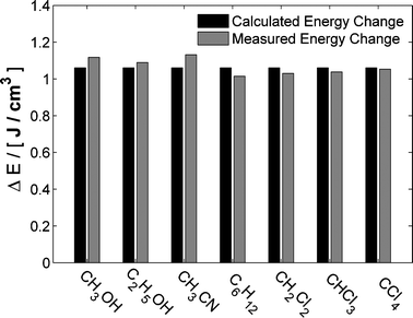
Changing the excitation wavelength results in difference scattering curves of different amplitude, however, when scaled by the amount of energy deposited in the sample the signals become indistinguishable (Fig. 7). The amount of energy deposited in the sample can be calculated from both steady-state variable temperature data, and directly by using the optical density of the dye solution together with the laser fluency as described in Section 3.4. The energy deposition calculated using an optical density of 0.15 is compared to the results of scaling the data to steady-state measurements in Fig. 8. The amount of deposited energy estimated from the two methods is within 5% of each other for all solvents studied.¹⁰¹ This shows that, when staying within the linear regime of the laser power, the absolute temperature change can be calculated directly from the spectroscopic parameters of the setup. Thus, the steady-state measurements at different temperatures become redundant. By using one of the azo-dyes, the solvent term described by eqn (4) can be determined on an absolute scale in a single TRWAXS experiment using only two time delays, 100 ps and 1 μs.

Fig. 7 100 ps (A) and 1 μs (B) difference scattering curves scaled to the 400 nm signal obtained for dye mediated solvent heating using 1 mM 4-bromo-4′-(N,N-diethylamino)-azobenzene (2) in acetonitrile and exciting at 400 nm, 475 nm and 518 nm. The recorded difference scattering curves are identical within the noise. All data have been recorded with 200 μJ (0.15 J cm⁻²) per pulse.

Fig. 8 Energy deposited in the solvent per unit volume in a laser pump, X-ray probe TRWAXS dye mediated solvent heating experiment calculated from the molar absorptivity and concentration of the dye (black) and determined from comparison with steady-state variable temperature experiments (grey).

4.2.4 Heating method. To confirm that the solvent response is independent of the heating method, the difference scattering responses resulting from dye mediated solvent heating and NIR heating of acetonitrile and methanol were compared. The normalized difference scattering curves are shown in Fig. 9. It has previously been shown that NIR excitation of methanol, at intermediate laser powers, gives a better description of solute mediated heat deposition than MD simulations.⁴⁸ Panel A in Fig. 9 shows that for methanol, NIR and dye-mediated solvent heating results in identical difference scattering curves. This demonstrates that the solvent response can be recorded with both mechanisms of energy deposition, and that the structural dynamics of the dye molecules does not contribute to the difference signal. For NIR mediated energy deposition in methanol, a fluency threshold of ∼1 J cm⁻² (∼800 GW cm⁻²) has been identified, above which a signature corresponding to a density increase contributes to the difference scattering signal from t < 50 ps to t = 2 ns.¹⁰² This short-lived density increase has been assigned to micro-cavitation (formation of micro-bubbles) in the liquid caused by extreme local heat deposition by higher-order absorption processes.

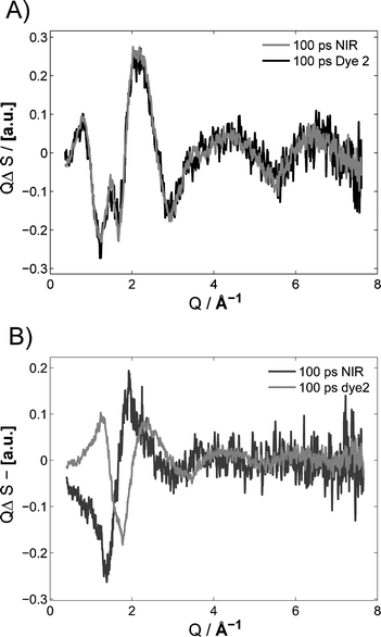Fig. 9 Normalized difference scattering curves of methanol (A) and acetonitrile (B) recorded with Δt = 100 ps following direct vibrational NIR excitation at 1718 nm (black) and dye-mediated heating with 4-bromo-4′-(N,N-diethylamino)-azobenzene (2, black). Laser power was 400 μJ (0.30 J cm⁻²) per pulse at 1718 nm, and 200 μJ (0.15 J cm⁻²) per pulse at 400 nm.

Panel B in Fig. 9 shows that a similar behaviour is observed for acetonitrile, with a significantly lower fluency threshold. As for methanol, the NIR mediated solvent heating results in difference scattering curves with a significant contribution of positive density change at the times up to t = 1 ns. The process of identifying the contribution as a result of a density increase is described in the ESI.† A cursory inspection shows that the NIR generated trace in panel B of Fig. 9 appears like a negative version of density differential in panel A of Fig. 5. Unlike methanol, the contribution from the density increase could be seen after NIR excitation of acetonitrile for all fluencies, where difference scattering signals could be detected. The minimum fluency where a difference scattering signal could be identified with NIR excitation of vibrational overtones of acetonitrile was 0.15 J cm⁻² (120 GW cm⁻²). We tentatively assign the lower fluency threshold for acetonitrile to an increased excited state absorption. This shows that NIR mediated energy deposition cannot be used to obtain the temperature component of the solvent differential for acetonitrile.

As the dependency on fluency and the fluency threshold is different from solvent to solvent, a scan of laser power has to be performed, when using NIR mediated solvent heating. This has to be done in order to verify that the solvent response is recorded at a laser power below the onset of any high-fluency effects. With the set-up used in these experiements, the transient signal recorded using NIR excitation of acetonitrile was monitored as the laser power was decreased to the point where no difference signal could be identified, even the least intense signal was dominated by high-fluency effects.

5 Conclusions

A set of three azo-dyes (1, 2 and 3) has been investigated in order to introduce a standardised method for experimental determination of the solvent response in laser-pump, X-ray probe time-resolved wide-angle X-ray scattering experiments on molecular systems in solution. The photophysics of the parent azobenzene compound were reviewed and we can conclude that on current synchrotron time scales (t > 50 ps) all energy from excitation of the dyes1–3 will have been deposited into the solvent as heat, and no other effects will be contributed to the difference scattering signal. The energy deposited in the solvent by dye-mediated solvent heating was shown to depend linearly on laser power and dye concentration. The magnitude of the difference scattering signal can be forced into a non-linear regime, but the shape of the measured difference scattering curve corresponding to a specific Δt remains unchanged. We must conclude that a difference scattering curve corresponding to point heating of the solvent can be obtained under a very wide range of experimental conditions; that is, dyes1–3 are ideal dye candidates to be used in a standardized method for experimental determination of the solvent term using dye mediated solvent heating. Complications inherent to NIR heating of the solvent, as observed in both methanol and acetonitrile, suggest that although NIR heating can be used to determine the solvent term, a standardized method has to use dye-mediated solvent heating. Furthermore, dye-mediated solvent heating allows for direct calculation of the amount of energy deposited in the solvent, thus removing the need for steady-state measurements. We have used the method proposed here to generate a library of the hydrodynamic constants and solvent differentials that constitute the solvent term in laser-pump, X-ray probe time-resolved wide-angle X-ray scattering experiments on systems in solution.⁵⁶

We conclude that the currently superior method for determining the solvent terms in a TRWAXS experiment is to use one of the dyes introduced here. The dyes are soluble in all solvents, they cover most of the visible spectrum, they give reproducible results on multiple beamlines,¹⁰³ they exhibit linear behaviour in a large concentration and laser power range, and they are readily available in pure form.⁵⁷ If a solution of one of these azo standards with a concentration corresponding to an optical density of 0.3 and a laser power lower than 200 μJ per pulse is used, then a pure solvent signal will be obtained in all laser pump X-ray probe TRWAXS experiments. A detailed description of how to obtain the solvent differentials is given in Appendix A and expanded in the ESI.†

Appendix

Appendix A: how to measure a solvent response

A solution of one of the three selected dyes should be prepared such that the optical density of the solution at the wavelength of the pump laser is 0.15–0.5. The laser peak fluency should be in the high end of the linear regime at around 0.2 J cm⁻². For a typical 300 μm liquid sheet, the energy-deposition should thus amount to around 5 J cm⁻³, and around 15 J cm⁻³ for a 100 μm liquid sheet. These are ‘typical’ experimental values and should give standard signal to noise ratios. Typically, only two time-delays are needed. One delay before the onset of the thermal expansion and one after the thermal expansion has run to completion (t ≪ L/v and t ≫ L/v, as described in the main text). Usually, a delay in the 100–500 ps range and a delay in the 1–3 μs range are used.

The early time point will contain the signal from the temperature change caused by the energy deposition at constant volume (ΔT = ΔE/C_V). While the late time-point will contain the signal from the temperature and density change experienced by the probe pulse after the thermal expansion has run its course (ΔT = ΔE/C_P, Δρ = α_VΔE/C_P). Thus, a linear combination of these two difference scattering curves can be used to describe any change in hydrodynamic parameters of the bulk solvent, and will be able to describe the solvent at any time-point during an experiment. The absolute value of heat and density change can be obtained, either through a steady-state experiment or by evaluating the deposited energy experienced by the X-ray probe pulse (both methods are described in the main text).

If NIR excitation is preferred, a wavelength should be chosen where the optical density of the sample is greater than 0.1 and the laser fluency should be adjusted to the optical density such that the initial temperature increase is no larger than 1.5 K. This will in most cases ensure that the data are recorded at a laser power lower than the breakdown of the linear response, although this might not be possible for all solvents (e.g.acetonitrile as shown in the main text). For an expanded description and a summarized experimental log see the ESI.†

Appendix B: description of the ID09B setup

Optical pump pulses were generated by frequency conversion of the fundamental radiation from the Legend Elite Ti:sapphire amplified system (Coherent Inc.) configured to produce picosecond near-IR pulses (802 nm, ∼1.2 ps FWHM), with the amplifier synchronized to the 360th subharmonic of the synchrotron RF clock (986.3 Hz). Frequency conversion was performed either by optical parametric amplification (TOPAS-800, LightConversion) or second harmonic generation. After frequency conversion the laser pulses were guided to the sample, arriving at a 10° inclination angle with respect to the incoming X-ray beam.

Single X-ray pulses (∼100 ps FWHM) generated from the U17 undulator were selected using a mechanical chopper, which – like the laser amplifier – was synchronized to the 360th subharmonic of the synchrotron orbit clock (986.3 Hz). For the measurements of the signal strength as a function of dye concentration and laser power, the raw pink-beam energy spectrum of the U17 undulator was used. For the rest of the measurements the X-ray energy-range was selected using a Ru-multilayer. For these measurements the energy spectrum of the X-ray pulses arriving at the sample is nearly perfectly Gaussian centered at 18.0 keV with a bandwidth of 2.5%. The sizes of the laser and X-ray focus were measured using a pinhole and determined to be 350 μm (h) × 340 μm (v) for the laser spot and 120 μm (h) × 80 μm (v) for the X-rays (horizontal and vertical dimensions respectively).

Before starting the experiment, a coarse timing (∼70 ps) of the laser/X-ray delay was determined by a GaAs diode placed just behind the sample system. During the experiment, the actual pump–probe delay on the sample was monitored non-invasively (∼10 ps precision) using a GaAs photo-diode capturing the laser scattering from one of the guiding mirrors and a fast diamond X-ray detector set in the direct beam transmitting about 90% of the radiation. The timing jitter was determined to be <2 ps (rms). The scattered X-rays were detected by a FreLON CCD detector with 2048 × 2048 pixels placed 45 mm from the liquid sheet sample produced by a high pressure nozzle.

Acknowledgements

The authors thank the Danish National Research Foundation's Centre for Molecular Movies, ESRF and DANSCATT for financial support, and Carlsbergfondet and the Villum Foundation for support for KH.

Notes and references

1. V. Srajer, T. Y. Teng, T. Ursby, C. Pradervand, Z. Ren, S. Adachi, W. Schildkamp, D. Bourgeois, M. Wulff and K. Moffat, Science, 1996, 274, 1726–1729.
2. B. Perman, V. Srajer, Z. Ren, T. Y. Teng, C. Pradervand, T. Ursby, D. Bourgeois, F. Schotte, M. Wulff, R. Kort, K. Hellingwerf and K. Moffat, Science, 1998, 279, 1946–1950.
3. C. Rischel, A. Rousse, I. Uschmann, P. A. Albouy, J. P. Geindre, P. Audebert, J. C. Gauthier, E. Forster, J. L. Martin and A. Antonetti, Nature, 1997, 390, 490–492.
4. D. A. Reis, M. F. DeCamp, P. H. Bucksbaum, R. Clarke, E. Dufresne, M. Hertlein, R. Merlin, R. Falcone, H. Kapteyn, M. M. Murnane, J. Larsson, T. Missalla and J. S. Wark, Phys. Rev. Lett., 2001, 86, 3072–3075.
5. A. Rousse, C. Rischel, S. Fourmaux, I. Uschmann, S. Sebban, G. Grillon, P. Balcou, E. Foster, J. P. Geindre, P. Audebert, J. C. Gauthier and D. Hulin, Nature, 2001, 410, 65–68.
6. S. Techert, F. Schotte and M. Wulff, Phys. Rev. Lett., 2001, 86, 2030–2033.
7. F. Schotte, M. H. Lim, T. A. Jackson, A. V. Smirnov, J. Soman, J. S. Olson, G. N. Phillips, M. Wulff and P. A. Anfinrud, Science, 2003, 300, 1944–1947.
8. M. Lorenc, J. Hebert, N. Moisan, E. Trzop, M. Servol, M. Buron-Le Cointe, H. Cailleau, M. L. Boillot, E. Pontecorvo, M. Wulff, S. Koshihara and E. Collet, Phys. Rev. Lett., 2009, 103, 028301.
9. S. O. Mariager, D. Khakhulin, H. T. Lemke, K. S. Kjaer, L. Guerin, L. Nuccio, C. B. Sorensen, M. M. Nielsen and R. Feidenhans'l, Nano Lett., 2010, 10, 2461–2465.
10. G. Dixit, O. Vendrell and R. Santra, Proc. Natl. Acad. Sci. U. S. A., 2012, 109, 11636–11640.
11. T. J. Penfold, I. Tavernelli, R. Abela, M. Chergui and U. Rothlisberger, New J. Phys., 2012, 14, 113002.
12. G. Dixit and R. Santra, J. Chem. Phys., 2013, 138, 134311–134319.
13. A. Aquila, M. S. Hunter, R. B. Doak, R. A. Kirian, P. Fromme, T. A. White, J. Andreasson, D. Arnlund, S. A. Bajt, T. R. M. Barends, M. Barthelmess, M. J. Bogan, C. Bostedt, H. Bottin, J. D. Bozek, C. Caleman, N. Coppola, J. Davidsson, D. P. DePonte, V. Elser, S. W. Epp, B. Erk, H. Fleckenstein, L. Foucar, M. Frank, R. Fromme, H. Graafsma, I. Grotjohann, L. Gumprecht, J. Hajdu, C. Y. Hampton, A. Hartmann, R. Hartmann, S. Hau-Riege, G. Hauser, H. Hirsemann, P. Holl, J. M. Holton, A. Hömke, L. Johansson, N. Kimmel, S. Kassemeyer, F. Krasniqi, K.-U. Kühnel, M. Liang, L. Lomb, E. Malmerberg, S. Marchesini, A. V. Martin, F. R. N. C. Maia, M. Messerschmidt, K. Nass, C. Reich, R. Neutze, D. Rolles, B. Rudek, A. Rudenko, I. Schlichting, C. Schmidt, K. E. Schmidt, J. Schulz, M. M. Seibert, R. L. Shoeman, R. Sierra, H. Soltau, D. Starodub, F. Stellato, S. Stern, L. Strüder, N. Timneanu, J. Ullrich, X. Wang, G. J. Williams, G. Weidenspointner, U. Weierstall, C. Wunderer, A. Barty, J. C. H. Spence and H. N. Chapman, Opt. Express, 2012, 20, 2706–2716.
14. S. P. Hau-Riege, A. Graf, T. Döppner, R. A. London, J. Krzywinski, C. Fortmann, S. H. Glenzer, M. Frank, K. Sokolowski-Tinten, M. Messerschmidt, C. Bostedt, S. Schorb, J. A. Bradley, A. Lutman, D. Rolles, A. Rudenko and B. Rudek, Phys. Rev. Lett., 2012, 108, 217402.
15. B. Rudek, S.-K. Son, L. Foucar, S. W. Epp, B. Erk, R. Hartmann, M. Adolph, R. Andritschke, A. Aquila, N. Berrah, C. Bostedt, J. Bozek, N. Coppola, F. Filsinger, H. Gorke, T. Gorkhover, H. Graafsma, L. Gumprecht, A. Hartmann, G. Hauser, S. Herrmann, H. Hirsemann, P. Holl, A. Homke, L. Journel, C. Kaiser, N. Kimmel, F. Krasniqi, K.-U. Kuhnel, M. Matysek, M. Messerschmidt, D. Miesner, T. Moller, R. Moshammer, K. Nagaya, B. Nilsson, G. Potdevin, D. Pietschner, C. Reich, D. Rupp, G. Schaller, I. Schlichting, C. Schmidt, F. Schopper, S. Schorb, C.-D. Schroter, J. Schulz, M. Simon, H. Soltau, L. Struder, K. Ueda, G. Weidenspointner, R. Santra, J. Ullrich, A. Rudenko and D. Rolles, Nat. Photonics, 2012, 6, 858–865.
16. L. X. Chen, W. J. H. Jager, G. Jennings, D. J. Gosztola, A. Munkholm and J. P. Hessler, Science, 2001, 292, 262–264.
17. R. Neutze, R. Wouts, S. Techert, J. Davidsson, M. Kocsis, A. Kirrander, F. Schotte and N. Wulff, Phys. Rev. Lett., 2001, 87, 195508.
18. C. Bressler, M. Saes, M. Chergui, D. Grolimund, R. Abela and P. Pattison, J. Chem. Phys., 2002, 116, 2955–2966.
19. M. Saes, C. Bressler, R. Abela, D. Grolimund, S. L. Johnson, P. A. Heimann and M. Chergui, Phys. Rev. Lett., 2003, 90, 047403.
20. C. Bressler and M. Chergui, Chem. Rev., 2004, 104, 1781–1812.
21. H. Ihee, M. Lorenc, T. K. Kim, Q. Y. Kong, M. Cammarata, J. H. Lee, S. Bratos and M. Wulff, Science, 2005, 309, 1223–1227.
22. M. Cammarata, M. Levantino, F. Schotte, P. A. Anfinrud, F. Ewald, J. Choi, A. Cupane, M. Wulff and H. Ihee, Nat. Methods, 2008, 5, 881–886.
23. A. Plech, M. Wulff, S. Bratos, F. Mirloup, R. Vuilleumier, F. Schotte and P. A. Anfinrud, Phys. Rev. Lett., 2004, 92, 125505.
24. S. Bratos, F. Mirloup, R. Vuilleumier, M. Wulff and A. Plech, Chem. Phys., 2004, 304, 245–251.
25. C. Bressler, C. Milne, V. T. Pham, A. El Nahhas, R. M. van der Veen, W. Gawelda, S. Johnson, P. Beaud, D. Grolimund, M. Kaiser, C. N. Borca, G. Ingold, R. Abela and M. Chergui, Science, 2009, 323, 489–492.
26. H. Ihee, Acc. Chem. Res., 2009, 42, 356–366.
27. S. Bratos, F. Mirloup, R. Vuilleumier and M. Wulff, J. Chem. Phys., 2002, 116, 10615–10625.
28. Q. Kong, M. Wulff, J. H. Lee, S. Bratos and H. Ihee, J. Am. Chem. Soc., 2007, 129, 13584–13591.
29. J. Vincent, M. Andersson, M. Eklund, A. B. Wohri, M. Odelius, E. Malmerberg, Q. Kong, M. Wulff, R. Neutze and J. Davidsson, J. Chem. Phys., 2009, 130, 154502.
30. S. Bratos and M. Wulff, in Advances in Chemical Physics, ed. S. A. Rice, 2008, vol. 137, pp. 1–29.
31. M. Christensen, K. Haldrup, K. Bechgaard, R. Feidenhans'l, Q. Kong, M. Cammarata, M. Lo Russo, M. Wulff, N. Harrit and M. M. Nielsen, J. Am. Chem. Soc., 2009, 131, 502–508.
32. K. Haldrup, T. Harlang, M. Christensen, A. Dohn, T. B. van Driel, K. S. Kjaer, N. Harrit, J. Vibenholt, L. Guerin, M. Wulff and M. M. Nielsen, Inorg. Chem., 2011, 50, 9329–9336.
33. K. Haldrup, M. Christensen, M. Cammarata, Q. Kong, M. Wulff, S. O. Mariager, K. Bechgaard, R. Feidenhans'l, N. Harrit and M. M. Nielsen, Angew. Chem., Int. Ed., 2009, 48, 4180–4184.
34. M. Christensen, K. Haldrup, K. S. Kjaer, M. Cammarata, M. Wulff, K. Bechgaard, H. Weihe, N. H. Harrit and M. M. Nielsen, Phys. Chem. Chem. Phys., 2010, 12, 6921–6923.
35. K. Haldrup, M. Christensen and M. M. Nielsen, Acta Crystallogr., Sect. A: Found. Crystallogr., 2010, 66, 261–269.
36. H. Cailleau, M. Lorenc, L. Guerin, M. Servol, E. Collet and M. Buron-Le Cointe, Acta Crystallogr., Sect. A: Found. Crystallogr., 2010, 66, 189–197.
37. L. X. Chen, X. Zhang, J. V. Lockard, A. B. Stickrath, K. Attenkofer, G. Jennings and D.-J. Liu, Acta Crystallogr., Sect. A: Found. Crystallogr., 2010, 66, 240–251.
38. M. Chergui, Acta Crystallogr., Sect. A: Found. Crystallogr., 2010, 66, 229–239.
39. P. Coppens, J. Benedict, M. Messerschmidt, I. Novozhilova, T. Graber, Y.-S. Chen, I. Vorontsov, S. Scheins and S.-L. Zheng, Acta Crystallogr., Sect. A: Found. Crystallogr., 2010, 66, 179–188.
40. T. Elsaesser and M. Woerner, Acta Crystallogr., Sect. A: Found. Crystallogr., 2010, 66, 168–178.
41. S. L. Johnson, P. Beaud, E. Vorobeva, C. J. Milne, E. D. Murray, S. Fahy and G. Ingold, Acta Crystallogr., Sect. A: Found. Crystallogr., 2010, 66, 157–167.
42. J. Kim, K. H. Kim, J. H. Lee and H. Ihee, Acta Crystallogr., Sect. A: Found. Crystallogr., 2010, 66, 270–280.
43. Q. Kong, J. H. Lee, M. Lo Russo, T. K. Kim, M. Lorenc, M. Cammarata, S. Bratos, T. Buslaps, V. Honkimaki, H. Ihee and M. Wulff, Acta Crystallogr., Sect. A: Found. Crystallogr., 2010, 66, 252–260.
44. R. J. D. Miller, R. Ernstorfer, M. Harb, M. Gao, C. T. Hebeisen, H. Jean-Ruel, C. Lu, G. Moriena and G. Sciaini, Acta Crystallogr., Sect. A: Found. Crystallogr., 2010, 66, 137–156.
45. M. Schmidt, T. Graber, R. Henning and V. Srajer, Acta Crystallogr., Sect. A: Found. Crystallogr., 2010, 66, 198–206.
46. S. Westenhoff, E. Nazarenko, E. Malmerberg, J. Davidsson, G. Katona and R. Neutze, Acta Crystallogr., Sect. A: Found. Crystallogr., 2010, 66, 207–219.
47. Q. Kong, J. H. Lee, K. H. Kim, J. Kim, M. Wulff, H. Ihee and M. H. J. Koch, J. Am. Chem. Soc., 2010, 132, 2600–2607.
48. M. Cammarata, M. Lorenc, T. K. Kim, J. H. Lee, Q. Y. Kong, E. Pontecorvo, M. Lo Russo, G. Schiro, A. Cupane, M. Wulff and H. Ihee, J. Chem. Phys., 2006, 124, 124504.
49. K. Haldrup, G. Vankó, W. Gawelda, A. Galler, G. Doumy, A. M. March, E. P. Kanter, A. Bordage, A. Dohn, T. B. v. Driel, K. S. Kjær, H. T. Lemke, S. E. Canton, J. Uhlig, V. Sundstrom, L. Young, S. H. Southworth, M. M. Nielsen and C. Bressler, J. Phys. Chem. A, 2012, 116, 9878–9887.
50. G. Hura, J. M. Sorenson, R. M. Glaeser and T. Head-Gordon, J. Chem. Phys., 2000, 113, 9140–9148.
51. A. M. Lindenberg, Y. Acremann, D. P. Lowney, P. A. Heimann, T. K. Allison, T. Matthews and R. W. Falcone, J. Chem. Phys., 2005, 122, 204507.
52. P. Georgiou, J. Vincent, M. Andersson, A. B. Wohri, P. Gourdon, J. Poulsen, J. Davidsson and R. Neutze, J. Chem. Phys., 2006, 124, 234507.
53. Q. Kong, M. Wulff, S. Bratos, R. Vuilleumier, J. Kim and H. Ihee, J. Phys. Chem. A, 2006, 110, 11178–11187.
54. S. Ibrahimkutty, J. Kim, M. Cammarata, F. Ewald, J. Choi, H. Ihee and A. Plech, ACS Nano, 2011, 5, 3788–3794.
55. A. Plech, V. Kotaidis, M. Lorenc and J. Boneberg, Nat. Phys., 2006, 2, 44–47.
56. https://sites.google.com/site/trwaxs/ .
57. contact: TJS@chem.ku.dk.
58. S. Yin, H. Xu, W. Shi, Y. Gao, Y. Song and B. Z. Tang, Dyes Pigm., 2006, 71, 138–144.
59. J. Griffiths and K.-C. Feng, J. Mater. Chem., 1999, 9, 2333–2338.
60. H. T. Clarke and W. R. Kirner, Org. Synth., 1922, 2, 47.
61. Even though the ML-spectrum is a Gaussian with a 2.5% bandwidth, the difference in the resulting scattering signal are quite similar to a monochromatic spectrum as the smearing from the ‘tail’ of the undulator spectrum has been filtered out.
62. P. Hamm, S. M. Ohline and W. Zinth, J. Chem. Phys., 1997, 106, 519–529.
63. J. C. Deak, L. K. Iwaki and D. D. Dlott, J. Phys. Chem. A, 1998, 102, 8193–8201.
64. J. C. Deak, S. T. Rhea, L. K. Iwaki and D. D. Dlott, J. Phys. Chem. A, 2000, 104, 4866–4875.
65. B. Valeur, Molecular Fluorescence: Principles and Applications, Wiley-VCH, Weinheim, 2002.
66. The decay from the lowest electronically excited state to the ground state can occur via radiative (luminescence) or non-radiative processes (IC). In the case of a non-radiative decay, the process releases more energy into the solvent.
67. P. Bortolus and S. Monti, J. Phys. Chem., 1979, 83, 648–652.
68. T. Fujino and T. Tahara, J. Phys. Chem. A, 2000, 104, 4203–4210.
69. T. Fujino, S. Y. Arzhantsev and T. Tahara, J. Phys. Chem. A, 2001, 105, 8123–8129.
70. H. Satzger, S. Sporlein, C. Root, J. Wachtveitl, W. Zinth and P. Gilch, Chem. Phys. Lett., 2003, 372, 216–223.
71. C. W. Chang, Y. C. Lu, T. T. Wang and E. W. G. Diau, J. Am. Chem. Soc., 2004, 126, 10109–10118.
72. Y. C. Lu, E. W. G. Diau and H. Rau, J. Phys. Chem. A, 2005, 109, 2090–2099.
73. T. Cusati, G. Granucci and M. Persico, J. Am. Chem. Soc., 2011, 133, 5109–5123.
74. H. Zollinger, Color Chemistry, Wiley VCH, New York, 3rd edn, 2001.
75. C. Roldan-Carmona, A. M. Gonzalez-Delgado, A. Guerrero-Martinez, L. D. Cola, J. J. Giner-Casares, M. Perez-Morales, M. T. Martin-Romero and L. Camacho, Phys. Chem. Chem. Phys., 2011, 13, 2834–2841.
76. M. Terazima, M. Takezaki, S. Yamaguchi and N. Hirota, J. Chem. Phys., 1998, 109, 603–609.
77. K. Takeshita, N. Hirota and M. Terazima, J. Photochem. Photobiol., A, 2000, 134, 103–109.
78. C. Ridley, A. C. Stern, T. Green, R. DeVane, B. Space, J. Miksosvska and R. W. Larsen, Chem. Phys. Lett., 2006, 418, 137–141.
79. L. D. Landau and E. M. Lifshitz, Fluid Mechanics, Pergamon Press, Oxford, 2nd edn, 1987.
80. P. R. Longaker and M. M. Litvak, J. Appl. Phys., 1969, 40, 4033.
81. F. Mirloup, R. Vuilleumier, S. Bratos, M. Wulff and A. Plech, Femtochemistry and Femtobiology: Ultrafast Events in Molecular Sciences, Elsevier, New York, 2004.
82. S. Bratos and M. Wulff, in Advances in Chemical Physics, ed. S. A. Rice, 2008, vol. 136.
83. http://www.hbcpnetbase.com/ .
84. http://webbook.nist.gov/chemistry/fluid/ .
85. M. Nakamura, K. Chubachi, K. Tamura and S. Murakami, J. Chem. Thermodyn., 1993, 25, 1311–1318.
86. P. Georgiou, J. Vincent, M. Andersson, A. B. Wöhri, P. Gourdon, J. Poulsen, J. Davidsson and R. Neutze, J. Chem. Phys., 2006, 124, 234507.
87. J. Nath, J. Chem. Thermodyn., 1996, 28, 481–490.
88. D. Harrison and E. A. Moelwyn-Hughes, Proc. R. Soc. London, Ser. A, 1957, 239, 230–246.
89. G. V. Stepanov, K. A. Shakhbanov, I. M. Abdurakhmanov and L. V. Malysheva, Russ. J. Phys. Chem., 1992, 12, 1493–1494.
90. In order to obtain a usable signal-to-noise ratio within a reasonable amount of time, at least 3% of the laser pump pulse should be deposited in the sample. This amounts to a decrease in signal strength by an order of magnitude compared to these experiments, where 200 repetitions were needed to obtain a good statistics S/N ratio. 3% absorptivity of a 300 μm liquid sheet corresponds to an optical density of 0.4 cm⁻¹.
91. R. Rey and J. T. Hynes, J. Chem. Phys., 1996, 104, 2356–2368.
92. H. Graener, R. Zurl and M. Hofmann, J. Phys. Chem. B, 1997, 101, 1745–1749.
93. O. V. Boyarkin, T. R. Rizzo and D. S. Perry, J. Chem. Phys., 1999, 110, 11346–11358.
94. E. L. Sibert and R. Rey, J. Chem. Phys., 2002, 116, 237–257.
95. L. K. Iwaki and D. D. Dlott, J. Phys. Chem. A, 2000, 104, 9101–9112.
96. C. G. Elles, D. Bingemann, M. M. Heckscher and F. F. Crim, J. Chem. Phys., 2003, 118, 5587–5595.
97. O. V. Boyarkin, L. Lubich, R. D. F. Settle, D. S. Perry and T. R. Rizzo, J. Chem. Phys., 1997, 107, 8409–8422.
98. S. Ashihara, N. Huse, A. Espagne, E. T. J. Nibbering and T. Elsaesser, Chem. Phys. Lett., 2006, 424, 66–70.
99. J. Lindner, P. Vöhringer, M. S. Pshenichnikov, D. Cringus, D. A. Wiersma and M. Mostovoy, Chem. Phys. Lett., 2006, 421, 329–333.
100. H. E Fischer, A. C. Barnes and P. S. Salmon, Rep. Prog. Phys., 2006, 69, 233–299.
101. The energy-deposition in acetonitrile has been corrected for direct multi-photon excitation of the solvent. The energy-deposition from direct excitation of the solvent has been found by back-extrapolating the linear regression Fig. 6A to zero and subtracting the back-extrapolation of Fig. 6B at zero yielding an estimated energy deposition of 0.12 J cm⁻³. No evidence of excessive energy deposition was found for the remaining solvents.
102. E. Pontecorvo, PhD thesis, Universitá degli Studi di Roma, 2006.
103. Unpublished results.

---

Footnote

† Electronic supplementary information (ESI) available: Absorption spectra of dyes and neat solvents. See DOI: 10.1039/c3cp50751c

---