Theoretical aspects of dynamic nuclear polarization in the solid state – spin temperature and thermal mixing
Yonatan
Hovav
,
Akiva
Feintuch
and
Shimon
Vega
*
Weizmann Institute of Science, Rehovot, Israel. E-mail: shimon.vega@weizmann.ac.il
First published on 16th November 2012
Abstract
Dynamic nuclear polarization is a method which allows for a dramatic increase of the NMR signals due to polarization transfer between electrons and their neighboring nuclei, via microwave irradiation. These experiments have become popular in recent years due to the ability to create hyper-polarized chemically and biologically relevant molecules, in frozen glass forming mixtures containing free radicals. Three mechanisms have been proposed for the polarization transfer between electrons and their surrounding nuclei in such non-conducting samples: the solid effect and cross effect mechanisms, which are based on quantum mechanics and relaxation on small spin systems, and thermal mixing, which originates from the thermodynamic macroscopic notion of spin temperature. We have recently introduced a spin model, which is based on the density matrix formalism and includes relaxation, and applied it to study the solid effect and cross effect mechanisms on small spin systems. In this publication we use the same model to describe the thermal mixing mechanism, and the creation of spin temperature. This is obtained without relying on the spin temperature formalism. Simulations of small model systems are used on systems with homogeneously and inhomogeneously broadened EPR lines. For the case of a homogeneously broadened line we show that the nuclear enhancement results from the thermal mixing and solid effect mechanisms, and that spin temperatures are created in the system. In the inhomogeneous case the enhancements are attributed to the solid effect and cross effect mechanisms, but not thermal mixing.
1. Introduction
A major drawback of NMR is its inherently low signal-to-noise ratio. This is due to the small nuclear Zeeman energies relative to the thermal energies at the temperatures and magnetic fields used in most NMR experiments. The Zeeman energy of unpaired electrons is at least 660 times larger than that of the nuclei, and the same for their spin polarizations at high temperatures. One possible way of enhancing NMR signals is to induce a polarization transfer between electrons and their neighboring nuclei via microwave (MW) irradiation, an experiment that was termed Dynamic Nuclear Polarization (DNP). DNP was first suggested by Overhauser in 19531 and shown later in practice by Carver and Slichter.2 The Overhauser effect relies on relaxation mechanisms which are present in conducting solids and in liquid samples. A number of years later DNP was demonstrated on solid dielectrics, where irradiation of the electron–nuclear double quantum (DQ) or zero quantum (ZQ) transitions led to nuclear polarization enhancements. This type of DNP experiment, termed solid state DNP, has gained high popularity in recent years mainly due to its applications in modern solid state NMR, NMR of biological samples and MRI (see for example ref. 3–11). Currently, most DNP experiments are based on hyper-polarization at cryogenic temperatures, followed by rapid dissolution and measurements at ambient temperatures,12 or on solid state DNP on frozen samples rotating at the magic angle.13–15Solid state DNP signal enhancement can be achieved by applying continuous wave (cw) MW irradiation on samples containing stable radicals at low temperatures. In recent years these samples are typically composed of frozen glass forming solvents, in which the radicals and molecules of interest were dissolved. The underlying theory of the DNP enhancement process is based on a quantum description including spin relaxation.16 In general DNP processes involve many unpaired electrons and nuclei which are dipolar coupled and experience different relaxation mechanisms. In order to take the multi-spin character of DNP into account concepts such as polarization transfer via spin diffusion17 and the spin temperature formalism18,19 are used to describe the DNP signal enhancement process.
To describe solid state DNP experiments one can consider small model spin systems and simulate DNP effects using standard quantum mechanical (QM) approaches common in NMR and EPR, involving spin–spin and spin–lattice relaxation mechanisms. This QM approach has led to the description of the Solid Effect (SE) and Cross Effect (CE) DNP mechanisms. In the SE DNP mechanism the nuclear polarization enhancement results from irradiation of “forbidden” DQ or ZQ electron–nuclear transitions, that become allowed due to the electron–nuclear hyperfine interactions.20,21 Saturation of these transitions together with electron spin–lattice relaxation can lead to large polarizations. This basic mechanism can easily be demonstrated for a single electron–nuclear spin pair. Calculations involving the CE-DNP mechanism require at least a three-spin system composed of two electrons and a nucleus. For the CE process to occur the difference between the electron Larmor frequencies must be about equal to the nuclear Larmor frequency.22–25 This results in state mixing which makes MW irradiation on the DQ or ZQ transition, which under this condition coincides with the single quantum (SQ) transition of the second electron, very efficient, and can therefore result in higher enhancements. For large systems these DNP mechanisms were typically described by using phenomenological rate equations. Some new insight into the SE-DNP and CE-DNP processes has been gained recently using a QM description26 and performing numerical simulations on model systems involving several nuclei and electrons.27–30 In addition, important progress has been made in performing DNP enhancement calculations on spin systems containing large numbers of nuclei.31,32
One of the theoretical models describing solid state NMR in general, and DNP in particular, on large strongly coupled spin systems has been formulated based on the concept of spin temperature in the rotating frame.18 Since we will be dealing with the spin temperature description of small spin systems, we will present a brief outline of this concept and its application to DNP, leading to the Thermal Mixing (TM) mechanism. Using the spin temperature formalism one assumes that during long MW irradiation (on a time scale longer than the decoherence time)16 on the spin system the population distribution over the energy levels follows Boltzmann statistics, and it is therefore possible to describe the system in the rotating frame in terms of temperature coefficients. This was first introduced by Redfield,18 who concluded that at the strong-irradiation limit the state of the spin system is defined by a single spin temperature. Provotorov extended this concept to weakly-irradiated spin systems,19 and showed the need for two temperature coefficients related to the Zeeman and dipolar interactions. The system is then defined using simple rate equations for these temperatures. These rate equations rely on the high temperature approximation, where at thermal equilibrium the energy level populations are linearly dependent on the energy terms of the Hamiltonian.
The spin temperature concept was first applied in the context of DNP by Solomon,33 for the interpretation of SE-DNP experiments. This was done using the strong MW irradiation limit of Redfield's theory. Later on Provotorov's rate equations were applied to DNP, and a nuclear Zeeman temperature was added to the electron Zeeman and (non-Zeeman) dipolar temperatures.16,34,35 This was done for electron systems with homogeneously broadened EPR spectra. The role of the applied MW field in the spin thermodynamical descriptions is to cool the electron Zeeman heat bath and to connect it to the dipolar and nuclear Zeeman heat baths, via the excitation of allowed and forbidden transitions.16 Alternatively, the heat transfer between the electron dipolar and nuclear Zeeman heat reservoirs can be treated using relaxation processes.16,36
At low lattice temperatures, where the populations are not any more linearly dependent on the energies of the Hamiltonian, the above-mentioned spin temperature concept must be modified. Borghini35 introduced a spin temperature model for DNP at low temperature that also deals with interacting electrons with an inhomogeneously broadened EPR spectrum.34 In this model, derived in detail by Abragam and Goldman,16 a single electron packet is assumed to be affected and saturated by the MW irradiation, and the steady state temperatures are derived from rate equations for the energies of the system. This model assumes that the packets are connected via dipolar cross-relaxation.
Spin temperature and the TM mechanism have been extensively discussed in the literature, as for example in ref. 16, 34 and 37–39, and more recently in ref. 40, which offers a unique and broad perspective of these topics. Experimental evidence for the existence of TM can be found in these references and in references within. In particular we should mention de-Boer's contribution that showed how the Borghini model35 can be extended to reproduce experimental line-shapes of DNP spectra.38 Recently, Jannin et al.41,42 discussed the necessity of additional modifications of the model to reproduce the overall shape of proton DNP spectra of glass forming solvents with TEMPO radical while relying on the TM mechanism.
In a set of recent publications we have used the spin density operator formalism in Liouville space for dealing with SE-DNP and CE-DNP processes in small spin systems, as well as with DNP assisted spin diffusion for enhancing bulk nuclei.27–30 As a natural extension of this formalism we try here to demonstrate the TM-DNP mechanism using the same theoretical approach. This is done by considering model spin systems containing seven electrons and one nucleus. These systems are of course too small to really mimic the multi-radical interacting networks imbedded in the dipolar coupled nuclear systems in real solid solutions. However, they are large enough to demonstrate the presence of spin temperature coefficients, without a priori assuming their existence. These results offer an additional insight into the dynamics of nuclear spin cooling, in particular in the case of TM-DNP for systems with homogeneously broadened EPR line-shapes. Our simulations also suggest that in the case of inhomogeneous EPR line-shapes the standard TM mechanism cannot account for the nuclear polarization.
2. The spin system
2.1 The Hamiltonian
To investigate the TM-DNP mechanism using the same theoretical approach that we developed to describe the SE-DNP and the CE-DNP processes, we chose a simple spin system consisting of a cluster of Ne interacting electrons, coupled to a single nucleus. As we will show, this simple system has the necessary interactions and relaxation parameters that enable a spin temperature description of the system. In future studies it will be desired to extend the number of nuclei in our spin configurations. The interaction Hamiltonian of the {eNe – n} system, H0, can be divided into three terms: the electron Zeeman Hamiltonian Hez, the nuclear Zeeman Hamiltonian Hnz, and the rest of the Hamiltonian Hrest containing the anisotropic part of the electron Zeeman interaction, the electron–electron dipolar interaction, and the electron–nuclear hyperfine interaction. Thus in the laboratory frame (L) the Hamiltonian is given by:| HL0 = HLez + Hnz + Hrest. | (1) |
When the system is irradiated by a constant MW field, of intensity ω1 and at a frequency ωMW, this Hamiltonian is transformed to the MW rotating frame (R):
| HR0 = HRez + Hnz + Hrest. | (2) |
The different terms in these expressions are of the form43
 | (3) |
 | (4) |
 , the electron–electron dipole interaction coefficients Δab, and the secular and pseudo-secular electron–nuclear hyperfine interaction coefficients Az,an and A±an. In our spin systems the nucleus is positioned close to a single electron a = 1, with hyperfine coefficients that are smaller than ωn. Since Hrest commutes with
  , it has the same form in the laboratory and the rotating frame. The MW irradiation Hamiltonian in the rotating frame is given by
 | (5) |
As we have done in earlier publications,27–30 we first diagonalize the main Hamiltonian H0 before introducing relaxation parameters. The diagonalized Hamiltonian can be represented by
| Λf0 = Hfez + D−1(Hnz + He + He–e + He–n)D, | (6) |
 , and can be further divided into two sets depending on the state of the nucleus. While the former is well defined, the latter is not, since in the diagonalized frame the nuclear states become mixed. We will therefore define the nuclear state using an index σ = ±, which is determined by the sign of the matrix element
 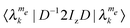 . When the nuclear state mixing is minor these elements will be approximately equal 1 for the nuclear spin up and −1 for the nuclear spin down, while for large state mixing some elements can become close to zero. As a result of this division we now deal with states
  , where k = 1,…,kme , and
  are all the states for a given me value and a given sign for σ. The energies of the
  states,
  , are indexed according to the Zeeman energy contributions meωe (for f = L) or meΔωe (for f = R) and the nuclear Zeeman contributions, which for small state mixing are about equal to ½σωn. The kme energies for each given me and σ value are spread by the anisotropic part of the electron Zeeman interaction, and the dipolar and hyperfine interactions.
2.2 The relaxation rates
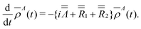
We can now introduce the spin–lattice relaxation rates of the system by defining single transition rates for all the transitions.27,28 To do so we realize that the populations of the spin system are equal to the diagonal elements of the spin density operator in the diagonalized representation,
 | (7) |
 . At thermal equilibrium these populations follow the Boltzmann statistics:
ρΛ(0) = Z![[thin space (1/6-em)]](https://www.rsc.org/images/entities/char_2009.gif) exp(−βLΛL0), exp(−βLΛL0), | (8) |
 | (9) |
The effect of the spin–lattice relaxation rates is to bring each pair of populations to its Boltzmann ratio  . The single transition rates are derived here from the electron and nuclear spin–lattice relaxation rates T−11e and T−11n, and are given by
 | (10) |
 | (11) |
 | (12) |
![[R with combining double overline]](https://www.rsc.org/images/entities/i_char_0052_033f.gif) 1, which affects the density operator in Liouville space, as will be described later.
1, which affects the density operator in Liouville space, as will be described later.
The spin–spin relaxation rates, defining the decay rates of the  coherences, are introduced here as a single T−12e rate for all transitions which are connected by a non-zero
  matrix element, and are therefore also affected by the MW Hamiltonian. A single T−12n rate is assigned to all other transitions. These rates compose the spin–spin relaxation super-operator 2.
2.3 The MW irradiation
After the transformation of the MW Hamiltonian to the diagonalized frame| ΛRMW = D−1HRMWD | (13) |
 ,
,  . These matrix elements can represent effective SQ irradiation fields, affecting
  transitions with σ = σ′, DQ fields, affecting
  transitions, or ZQ fields, affecting
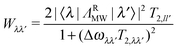
 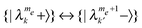 transitions. Where the state mixing is small, as in the SE-DNP case, the SQ elements are of the order of ω1 and the DQ and ZQ elements are very small. However at the CE conditions,26,29 where the mixing becomes large, all three types of elements can be of the order of ω1.
All matrix elements of ΛR0 + ΛRMW can be transformed to the super-operator  in Liouville space and added to the 1 and 2 relaxation super-operators. The time dependence of the density operator vector in Liouville space can then be calculated by solving27,28
 | (14) |
 | (15) |
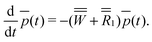
These rates can be combined to form the ![[W with combining double overline]](https://www.rsc.org/images/entities/i_char_0057_033f.gif) matrix that together with the spin–lattice relaxation super-operator 1 determines the evolution of the vector
matrix that together with the spin–lattice relaxation super-operator 1 determines the evolution of the vector ![[p with combining macron]](https://www.rsc.org/images/entities/i_char_0070_0304.gif) (t), composed of all
(t), composed of all  populations, according to:
 | (16) |
The time dependence of the polarizations of each electron a and of the nucleus n can then be calculated using:
 | (17) |
These can be normalized with respect to the electron thermal equilibrium polarization
 | (18) |
 is given by eqn (7) and (8).
Using the population rate equation given in eqn (16) we have ignored all coherent effects in the system and over-simplified the short time behavior of the system (on the order of T2e or less). Although this might be significant when dealing with large MW irradiation fields, in what follows we will use this approach for all simulations in order to increase the maximum possible number of spins in our model systems.
As mentioned in the introduction, DNP simulations on larger spin systems were already performed by Karabanov et al.32 using Krylov–Bogolyubov time averaging. This important approach was applied to simulate the dynamics of SE-DNP enhancement experiments on a system containing a single electron and 25 nuclei. An extension involving the CE-DNP mechanism in a three-spin system was recently presented as well.44 Future extensions of Karabanov's approach, involving several strongly coupled electrons or electrons with a large spread of resonance frequencies, will make it possible to treat systems similar to the ones discussed here.
2.4 Spin temperature
Before presenting the simulation results, we repeat here some of the basic principles of the spin temperature concept16,18,19,35 that are relevant for our analysis. In order to describe the DNP mechanism using this concept we must be able to express the populations of our system in terms of a set of spin temperature coefficients. When the populations of a spin system with a diagonal Hamiltonian Λ0 are defined by a single inverse temperature coefficient βL, the population vector can be written as | (19) |
 in the laboratory frame. In our spin systems this vector can be decomposed according to
| ĒL = [[HLez] + [[D−1(Hnz+Hrest)D]], | (20) |
 diagonalized frame. The first vector is defined by the isotropic parts of the electron Zeeman energies meωe and the second vector of all other energy contributions. In the same way the energy vector in the rotating frame can be written as
| ĒR = [[HRez] + [[D−1(Hnz+Hrest)D]], | (21) |
 | (22) |
 | (23) |
Here the first term in the exponent represents the contribution of the electron Zeeman Hamiltonian to the populations and the second term the contributions from the rest of the Hamiltonian. In the high temperature approximation we can write
 | (24) |
 with a fixed me value, and a rotating frame temperature for the average populations of these manifolds.
The spin temperature concept can now be expanded and the assumption can be made that during an applied MW irradiation field of duration longer than T2 the population vector can be defined in terms of three time dependent temperature coefficients: the electron Zeeman βfez, the nuclear Zeeman βnz, and the rest βrest:
| (t) ≃ p−10(1 − βRez(t)[[HRez]] − βnz(t)[[D−1HnzD]]) + βrest(t)[[D−1(He+He–e+He–n)D]] | (25) |
(t). This can be justified as long as the hyperfine induced state mixing is weak, |A±an| ≪ |ωn|. When βnz(t) = βrest(t) the off-diagonal elements cancel out and eqn (25) has the same form as eqn (24). The contributions to (t) from the nuclear Zeeman interaction [[D−1HnD]] elements are proportional to −½ωn or ½ωn. The main contribution from the [[D−1(He + He–e + He–n)D]] elements depends on the type of the system considered: for systems with ||He–e|| ≫ ||He||,||He–n|| it is mainly proportional to the strength of the electron dipolar interactions, and βdip will be used instead of βrest; when ||He|| ≫ ||He–e||,||He–n|| it is proportional to the anisotropic part of the Zeeman interaction, δa, and we will denote βrest as the g-distribution temperature βg.
At this point it is helpful to present the expressions for (t) graphically. According to eqn (25), each group of populations  with fixed values for me and σ should show a linear energy dependence with a slope proportional to βrest. The average values of the populations of these groups should also be linear with energy with a slope proportional to βez. Finally, to show the existence of a nuclear temperature we must monitor the slopes of the lines through the 2Ne pairs of populations
  and
and  that contribute to the nuclear signal. A well-defined nuclear spin temperature means that in a population–energy diagram the majority of these lines are parallel, with a slope proportional to βnz. Thus, the creation of a single nuclear temperature, even for a single nucleus in our spin systems, is not necessarily a trivial issue.
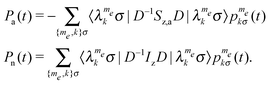
Fig. 1 shows the energy diagram of two spin systems, containing seven interacting electrons and one nucleus, at thermal equilibrium. The Larmor frequency of the electrons in both systems is about 9.9 GHz and the nuclear Larmor frequencies are equal to ωn/2π = 1.5 MHz or 15 MHz, where the latter is the proton frequency in the field of 0.35 Tesla. Here all δa shifts were set to zero, and all electrons are dipolar coupled to one another, resulting in a homogeneously broadened EPR spectrum. In Fig. 1a the laboratory frame diagrams are plotted for both spin systems. Each of the energy bands shown in the figure has a single me value and an average energy value equal to meωe. The number of levels within each of the me manifolds is indicated above each of the energy bands, as well as the number of electrons being in state α or β position in this manifold, as indicated by (nα,nβ), with me = ½(nα − nβ). Blow-ups of the energy distributions around ½ωe/2π ≈ 5 GHz are shown (not to scale) in Fig. 1b and c for the systems with ωn/2π = 1.5 MHz and 15 MHz, respectively. For both cases states corresponding to σ = + are plotted in red and to σ = − in black. These two types of σ-states differ in energy by about ωn.
 | ||
Fig. 1 Laboratory frame energy level diagrams of two homogeneously broadened systems each containing seven electrons and a single nucleus with nuclear Larmor frequencies equal to ωn/2π = 1.5 or 15 MHz. All other parameters of the systems are given in Table 1. The full diagram is shown in (a) and is at a resolution on the scale of the electron Larmor frequency ωe ≃ 9.9 GHz, in which case both systems look the same. Each of the lines in (a) corresponds to an energy band with a given me value, containing a total number  of energy levels with nα electrons in state α and nβ in β, indicated above each band as of energy levels with nα electrons in state α and nβ in β, indicated above each band as  . The me = ½ band is shown at a high energy resolution in (b) and (c) for the systems with ωn/2π = 1.5 and 15 MHz, respectively. The black and red energy lines indicate states with σ = −, +, which correspond to nuclear states close to the β and α product states, respectively. These two groups of state are shifted by about ωn, as indicated in the figure. The separation of energy levels within the same me and σ values is caused mainly by the electron dipolar interaction. . The me = ½ band is shown at a high energy resolution in (b) and (c) for the systems with ωn/2π = 1.5 and 15 MHz, respectively. The black and red energy lines indicate states with σ = −, +, which correspond to nuclear states close to the β and α product states, respectively. These two groups of state are shifted by about ωn, as indicated in the figure. The separation of energy levels within the same me and σ values is caused mainly by the electron dipolar interaction. | ||
In Fig. 2 the population–energy diagrams of the two systems described above are shown. Here the points defining the energy and population of each state are plotted as red circles (σ = +) and black dots (σ = −). In Fig. 2a the laboratory frame diagrams are plotted for both spin systems. Blow-ups of their population distributions around 5 GHz (marked by the dashed box) are shown in Fig. 2d and e. Projections of the population–energy points in Fig. 2a, d and e onto the energy axis (y-axis) result in the diagrams shown in Fig. 1a–c, respectively. All populations in Fig. 2a show a linear dependence on the energy with a constant slope, indicating that all temperatures in the systems are equal to the lattice temperature, chosen to be 10 K. Small deviations from linearity are due to high order terms of the Taylor expansion in eqn (19). In the following we will ignore these small deviations and analyze our results, assuming the high temperature approximation. Fig. 2b shows the Δωe/2π = −4 MHz rotating frame diagram of the ωn/2π = 1.5 MHz nucleus, and Fig. 2c the Δωe/2π = −15 MHz rotating frame diagram of the ωn/2π = 15 MHz nucleus. In these frames the electron spin temperatures TRe become equal to about 4 mK and 15 mK, respectively, and the slopes in Fig. 2b and c differ from that in Fig. 2a. The nuclear Zeeman Tzn and dipolar Tdip temperature remains at 10 K, and their distribution within each me state is the same as in Fig. 2a. Therefore the areas marked by the dashed boxes in Fig. 2b and c are the same as the population distributions shown in Fig. 2d and e.
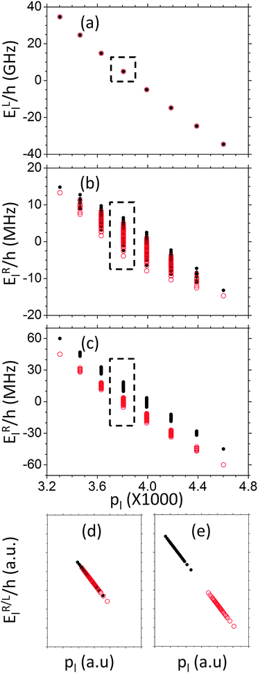 | ||
| Fig. 2 Thermal equilibrium population vs. energy diagrams of the homogeneously broadened systems used in Fig. 1, with ωn/2π = 1.5 or 15 MHz. In (a) this is shown for both systems in the laboratory frame while in (b) and (c) they are shown in the rotating frame separately for ωn/2π = 1.5 MHz or 15 MHz, respectively. In (d) and (e) a blow-up of a region in the diagrams is shown, as marked by the dashed lines in (a) and (b) or (a) and (c), respectively. The black dots and red circles correspond to states with σ = ∓, respectively. | ||
The application of a cw MW irradiation is assumed not to change the energies in our diagonal representation, but it can (partially) equalize populations of states with similar rotating frame energies, and together with the relaxation mechanisms will result in some new steady state distribution of the whole system.
In the next sections we will follow the values of the populations and polarizations of our model systems by solving the rate equation given in eqn (16). This will be done for systems with either a homogeneously or an inhomogeneously broadened EPR line. By plotting polarization-energy diagrams as a function of time we can show the appearance of the spin temperatures, and calculate their time evolution. Frequency swept DNP spectra will also be shown for different spin systems and for varying MW irradiation powers.
3. Electrons with a homogeneously broadened EPR spectrum
In this section we consider a system with a homogeneously broadened EPR line, where the unsaturated line-shape is mainly determined by the electron dipolar interaction. Thus we neglect the anisotropic part of the electron Zeeman interaction, and set δa = 0 for all electrons, such that He = 0. In these systems the flip–flop terms of the dipolar interaction in He–e are not quenched by the electron frequency distributions, and in the spin temperature picture the system is defined by βez, βnz and βdip, where the last is mainly determined by the dipolar interactions.At first we describe how the effect of the MW irradiation and spin–lattice relaxation on the populations is influenced by the electron dipolar interactions, while ignoring the presence of the nucleus and thus of the σ index. The dipolar interactions result in large electron state mixing in the diagonalized Hamiltonian (eqn (6)) and have a large effect on both the magnitudes and the distribution of the relaxation and MW rates between states. The T1e spin–lattice rates, derived from eqn (10), will connect pairs of  states, with each k state coupled to many k′ states, and vice versa. These rates create Boltzmann distributions between levels with Δme = ±1, and in addition between levels with the same me value. The MW Hamiltonian in the diagonalized frame (eqn (13)) has many effective SQ transition rates Wλλ′ (eqn (15)), with |λ〉 and |λ′〉 respectively belonging to
  and
and  manifolds of states, and can equalize populations when they have similar rotating frame energies. Therefore, the populations of some {me} states will approach those of {me + 1} and other {me} populations will get close to those of {me − 1}, depending on the choice of the rotating frame.
Reintroducing the nucleus to the spin system, the diagonalization of the Hamiltonian results in Wλλ′ and T1,λλ′ rates of |λ〉–|λ′〉 transitions, which can be SQ transitions of the form  or DQ and ZQ transitions of the form
  . The degree of state mixing and the magnitudes of the effective Wλλ′ and T1,λλ′ rates of the SQ, DQ and ZQ transitions depend strongly on the size of the nuclear Zeeman interaction with respect to the electron dipolar interactions. It is therefore convenient to consider two types of systems:
(I) Systems in which the dipolar broadened energy bands corresponding to the states  and
and  overlap. In this case we expect a strong state mixing involving the nuclear spin states, in analogy to the state mixing in the CE case. Then the MW irradiation can simultaneously excite SQ and DQ or ZQ transitions, and the T1e relaxation mechanism will result in significant electron–nucleus cross-relaxation.29,45,46 These conditions are relevant when ωn is smaller than the width of the electron dipolar broadened EPR line width, and we can expect that the nuclear polarization will be a result of the TM-DNP mechanism.16,34 A population–energy diagram for such a system at thermal equilibrium is shown in Fig. 2a and b.
(II) Systems in which the energy bands of  and
and  do not overlap. This results in only minor mixing between states with different nuclear states, as in the SE case. Here the MW irradiation can excite DQ or ZQ transitions without exciting SQ transitions, and the T−11e driven electron–nuclear cross-relaxation rates will be small. This situation corresponds to systems where ωn is larger than the electron EPR line, and the nuclear enhancement results from SE-DNP mechanisms.16,34 An example of a population–energy diagram of such a system at its thermal equilibrium is shown in Fig. 2a and c.
Our simulations provide the values of the population vector (t) in the diagonalized frame. If we assume that eqn (25) defines this vector at any time, we can derive the value of the three spin temperatures using:
| βRez (t) ≅−p0((t)·[[HRez]])/([[HRez]]·[[HRez]]) |
| βnz(t) ≅−p0((t)·[[D−1HnzD]])/([[D−1HnzD]]·[[D−1HnzD]]) |
| βdip(t) ≅−p0((t)·[[D−1HdipD]])/([[D−1HdipD]]·[[D−1HdipD]]). | (26) |
These expressions are derived by taking the dot product of (t) in eqn (25) with [[HRez]], [[D−1HnD]], or [[D−1HDD]], while assuming that
| |[[D−1HnzD]]·[[D−1HdipD]]| ≪ |[[D−1HnzD]]·[[D−1HnzD]]|, |[[D−1HdipD]].[[D−1HdipD]]|. | (27) |
In what follows we will show simulated population distributions and their resulting polarizations. We first show the steady state DNP spectra obtained for different nuclear Larmor frequencies. We then consider the steady state and temporal evolution of the populations in a type (I) and type (II) system, and check whether the population–energy diagrams can be described using spin temperature coefficients. As before, black dots and red circles correspond to states with σ = − and σ = +, respectively. The interaction and relaxation parameters used in these simulations are summarized in Table 1, unless stated otherwise in the figure captions or in the text. We chose Az,1n to be zero in order to prevent partial quenching of the electron–electron interactions by the hyperfine interaction. We did not introduce electron–electron cross relaxation rates T−11D during these calculations, but relied on T−11e to generate finite rates.
| Parameter | Value |
|---|---|
| a Unless stated otherwise in the text and the figure caption. b This was calculated using electrons positioned, relative to electron e1, at [x,y,z] of [35,0,0], [0,38,0], [0,0,32] [36,30,0], [26,0,42] and [0,36,31], where z is the direction of the external magnetic field. | |
| ω 1H/2π | 15 MHz |
| ω 1/2πa | 100 kHz |
| δ a | 0 |
| D ab | >1.8 MHz |
| A z,an | 0 |
| A ±1n | ω n/15 |
| A ±(a≠1)n | 0 |
| T 1e | 10 ms |
| T 1n | 2 s |
| T 2e | 10 μs |
| T 2n | 1 ms |
| T L | 10 K |
3.1 The DNP spectra
Fig. 3 shows the frequency-swept DNP spectra of {e7–n} spin systems at their steady state. The steady state polarizations of the electrons at each MW frequency are also plotted in the figure (gray lines). Five different {7e–n} systems were considered with a nucleus having different nuclear gyromagnetic ratios. For a field of 0.35 Tesla the corresponding Larmor frequencies were chosen equal to 1.5, 3, 6, 12 and 15 MHz, with the latter corresponding to a 1H nucleus while the other frequencies do not correspond to existing nuclei. This choice enabled simulations using nuclei with Larmor frequencies smaller and larger than the width of the EPR line, while keeping the dipolar interaction strengths at about 1 MHz. In addition, relatively high ratios between the pseudo-hyperfine coefficient and the nuclear Larmor frequency were used by setting A+/ωn = 1/15 in all our calculations. With these values we obtained an efficient DNP mechanism even at relatively low MW powers and realistic relaxation times, resulting in the relatively smooth DNP profiles shown in this figure and in the following ones.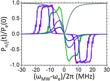 | ||
| Fig. 3 Steady state electron (gray) and nuclear polarization as a function of the cw MW irradiation frequency. This was done for homogeneously broadened systems composed of seven electrons and a single nucleus with ωn/2π = 1.5 MHz (dark blue), 3 MHz (light blue), 6 MHz (green), 12 MHz (purple) or 15 MHz (violet). All other parameters of the system are given in Table 1. | ||
For ωn/2π = 1.5 MHz (dark blue line) and 3 MHz (light blue line) the DNP spectra show positive–negative enhancement profiles which are confined inside the electron polarization saturation profile, with a width of ∼8 MHz. The resulting DNP spectra are almost identical, with the maximal enhancement proportional to the value of ωn, indicating that the nuclei with different ωn have the same nuclear Zeeman spin temperature Tnz. These features are typical for TM-DNP.40 For these two ωn/2π values we are dealing with systems of type (I), where the MW irradiation excites simultaneously SQ, DQ as well as ZQ transitions. No DNP enhancement is therefore expected outside the electron saturation profile.
For ωn/2π values larger than the width of the EPR line we observe a dramatic change in the DNP spectrum, as can be seen for ωn/2π = 12 MHz (purple line) and 15 MHz (violet line). Here the positive and negative enhancements are positioned around ωe ± ωn, as expected for the SE enhancement of systems of type (II), and with an almost full nuclear enhancement over a frequency range of 6 MHz. This line-shape is the result of the dipolar state mixing in this system.
For the intermediate value ωn/2π = 6 MHz (green line) the DNP spectrum shows two features: one spectrum which is four times higher than that of ωn/2π = 1.5 MHz, and has about the same shape as the spectra of the type (I) systems; and a DNP spectrum that has maximal polarizations around ±6 MHz, as for type (II) systems. This is a manifestation of the fact that in the present system there are DQ or ZQ transitions that do and do not overlap with SQ transitions.
In Fig. 4 the dependence of the steady state DNP spectra on the MW intensity ω1 is investigated. This was done for the two extreme ωn values only: in (a) for ωn/2π = 1.5 MHz, corresponding to a system of type (I); and in (b) for ωn/2π = 15 MHz, corresponding to a system of type (II). For the type (I) system increasing ω1/2π from 10 kHz to 400 kHz results in a broadening of the DNP spectrum. The maximal polarization initially increases with ω1, and then decays for higher values. These effects are due to a broadening of the MW excitation bandwidth, where the decay in the maximal polarization is due to simultaneous saturation of ZQ and DQ and to partial saturation of the electron polarization due to irradiation on SQ transitions. For the system with ωn/2π = 15 MHz the width and the overall shape of the DNP profile change only slightly for increasing MW power. Here again high MW irradiation intensities can result in a decrease of the end polarization, due to off resonance irradiation of the SQ transitions. In both cases, using ω1/2π = 10 kHz results in simulated DNP profiles that are no longer smooth, due to the small number of electrons in our spin system. We therefore use this value as a lower limit in the rest of the simulations.
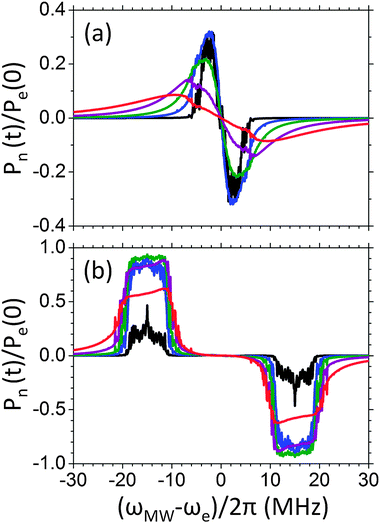 | ||
| Fig. 4 Steady state nuclear polarization as a function of the cw MW irradiation frequency, using MW power of 10 kHz (black), 50 kHz (blue), 100 kHz (green), 200 kHz (purple) and 400 kHz (red). This was done for homogeneously broadened systems composed of seven electrons and a single nucleus with ωn/2π = 1.5 MHz (a) or 15 MHz (b). All other parameters of the system are given in Table 1. | ||
The conclusion from these simulations is that our theoretical model applied on relatively small spin systems shows the characteristic features of TM-DNP and SE-DNP processes, as known from the literature. The question we must ask now is whether the simulated results are also consistent with the spin temperature description described above. In what follows we shall show that this is indeed the case and that discrete spin temperatures can be derived from population–energy diagrams by solving the rate equation in eqn (16).
3.2 Population–energy diagrams for a type (I) spin system – thermal mixing DNP
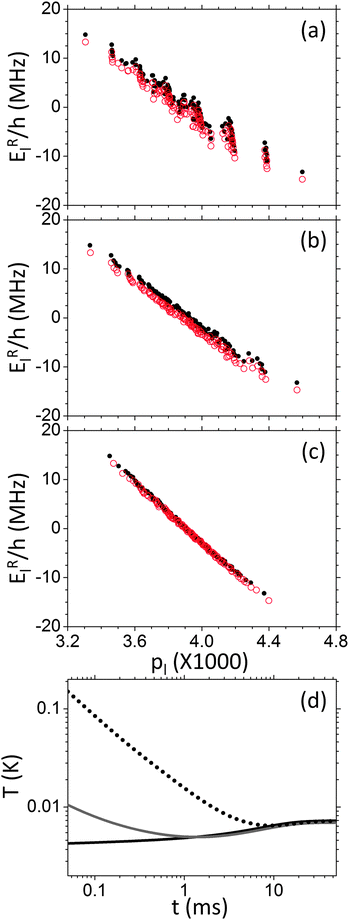
In this section we concentrate on a system with ωn/2π = 1.5 MHz, and with the MW irradiation applied at Δωe/2π = −4 MHz. The thermal equilibrium population–energy diagram of this system in the laboratory and rotating frame has been shown in Fig. 2a and b. Once again, the transfer to the rotating frame results in this case in TRez ≃ 4 mK and Tnz = Tdip = 10 K. Fig. 5a–c shows the steady state population–energy diagram during MW irradiation with a field strength of ω1/2π = 10, 100 or 400 kHz. For irradiation power of 100 and 400 kHz these diagrams show reasonably well-defined straight lines, with slopes corresponding to one common spin temperature (TRez = Tdip = Tnz) of about 7 mK and 40 mK, respectively. This indicates a significant cooling of the nuclear and dipolar baths and a slight heating of the electron Zeeman bath. For the low MW power level of 10 kHz the populations are not arranged according to straight lines and the three temperatures are not well defined.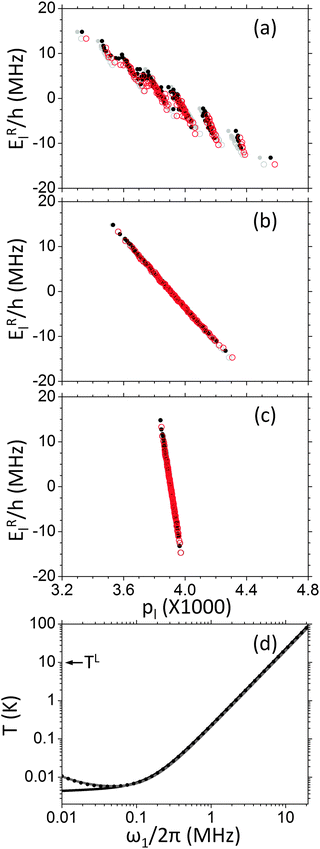 | ||
| Fig. 5 Steady state population vs. energy diagrams, for a homogeneously broadened system composed of seven electrons and a single nucleus with ωn/2π = 1.5 MHz. This was done using cw MW irradiation with a power of ω1/2π = 10 kHz (a), 100 kHz (b), or 400 kHz (c), and a MW frequency of (ΔωMW − ωe)/2π = −4 MHz. The black dots and red circles correspond to populations of states with σ = ∓1, respectively, and are a result of the simulation, while the gray dots and circles are the calculated energy-population relations for σ = ∓1, respectively, assuming the state of the system is given by three temperatures, as given in eqn (26). In (d) the steady state temperatures of the rotating frame electron Zeeman (solid black line), dipolar (gray line), and nuclear Zeeman (doted black line) baths are drawn as a function of the MW power. This was calculated from the populations using eqn (26). The lattice laboratory frame temperature is indicated by an arrow. All other parameters of the system are given in Table 1. | ||
We can also calculate the temperatures using the expressions in eqn (26), where we a priori assume that the populations are defined by three temperatures according to eqn (25). Doing so we obtained three temperatures, which we can use to reconstruct approximate polarization–energy diagrams, again using eqn (25). The results of this procedure (gray dots and circles for the σ = ∓states, respectively) are also shown in Fig. 5a–c. For the high MW powers there are only small deviations between the simulated and the approximated diagrams, and only at the extreme me values, showing that the high temperature approximation is valid. For an irradiation strength of 10 kHz these deviations become large.
In Fig. 5d we used eqn (26) to show the dependence of the three steady state spin temperatures on the MW power. Even when the temperatures are not well defined we can get some insight from these diagrams. Starting from ω1/2π = 10 kHz we see that Tnz and Tdip are about equal and approach TRez for increasing ω1 values. Interestingly, increasing the MW power leads to a common temperature that exceeds the laboratory temperature of 10 K. This indicates that the MW irradiation increases the total energy of the system, which is given by  , and therefore acts as a heat pump. This process is caused by the equilibration of population by off resonance irradiation, and is limited by the spin–lattice relaxation mechanism, trying to bring the system back to the lattice temperature. The effect of the spin–lattice mechanism is illustrated in Fig. 6, where the steady state population–energy diagrams are plotted for T1e = 1, 10 and 100 ms, and using ω1/2π = 100 kHz. Here we did not differentiate between the σ states, for simplicity. As can be seen, shortening T1e results in a lowering of the steady state temperature, bringing the electron Zeeman bath closer to its thermal equilibrium value.
 | ||
| Fig. 6 Steady state population vs. energy diagrams, for a homogeneously broadened system composed of seven electrons and a single nucleus with ωn/2π = 1.5 MHz. This was done using T1e of 1 ms (black circles), 10 ms (blue circles), or 100 ms (red circles), with the irradiation applied at (ΔωMW − ωe)/2π = −4 MHz. All other parameters of the system are given in Table 1. | ||
We can also follow the temporal evolution of the populations and the spin temperatures. In Fig. 7a–c population–energy diagrams are plotted for a 100 kHz MW irradiation field of durations tMW equal to 0.05 ms, 0.5 ms and 5 ms. The first corresponds to five times T2e. Initially, the MW irradiation affects the spin system in a way that cannot be described using the spin temperature expression in eqn (25). In this rotating frame the high energy levels in each of the me manifolds are drawn towards me − 1 states, and the low energy levels to me + 1 states. After 0.5 ms the diagram of the system can be characterized in terms of two parallel lines for the populations with σ = + and σ = −. The common slope of these lines corresponds to one temperature for TRez = Tdip. The lines connecting the populations  and
and  show approximately a single slope, which differs from the former slope, and therefore Tnz is not equal to TRez and Tdip. After tMW = 5 ms all temperatures become equal. This common temperature reaches its steady state value after about 50 ms, which is equal to five times T1e. In Fig. 7d we show the spin temperatures, again using eqn (26), as a function of the MW irradiation time tMW. The temperature equilibration process is driven by the MW irradiation, exciting simultaneously DQ and SQ transitions. It is therefore analogous to the CE-DNP mechanism, which also relies on simultaneous SQ and DQ/ZQ MW irradiation, and where the steady state of the core nuclei is also reached in a time scale of the order of T1e.29 That the dipolar temperature Tdip becomes equal to TRez in a timescale shorter then T1e is an indication that the excitation of the SQ transitions is much more efficient than that of the DQ ones.
 | ||
| Fig. 7 Population vs. energy diagrams at different times, for a homogeneously broadened system composed of seven electrons and a single nucleus with ωn/2π = 1.5 MHz. This was done using cw MW irradiation for a duration of 50 μs (a), 0.5 ms (b), or 5 ms, with the irradiation applied at (ΔωMW − ωe)/2π = −4 MHz. The black dots and red circles correspond to populations of states with σ = ∓1, respectively. In (d) the temperatures of the rotating frame electron Zeeman (solid black line), dipolar (gray line), and nuclear Zeeman (dashed black line) bath are drawn as a function time. This was calculated from the populations using eqn (26). All other parameters of the system are given in Table 1. | ||
3.3 Population–energy diagrams for a type (II) spin configuration – solid effect DNP
A similar set of simulations was performed on the type (II) spin system with ωn/2π = 15 MHz and Δωe/2π = −15 MHz. The thermal equilibrium plots of this system in the laboratory and rotating frames are shown in Fig. 2a and c. In Fig. 8a–c the steady state population–energy plots in the rotating frame are shown for MW irradiation fields of ω1/2π = 10, 100 and 400 kHz. In all cases there are well defined slopes corresponding to three spin temperatures. In Fig. 8d the steady state spin temperatures are shown as a function of ω1/2π, as derived from eqn (26). In this case the MW field equalizes Tnz and TRez, leaving Tdip at a higher value. For high MW intensities Tdip becomes approximately equal to Tnz ≃ TRez. Once again the temperatures can rise above the lattice temperature due to MW heating.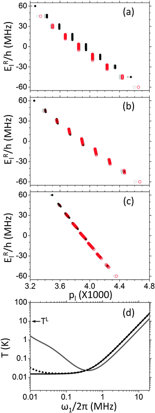 | ||
| Fig. 8 Steady state population vs. energy diagrams, for a homogeneously broadened system composed of seven electrons and a single nucleus with ωn/2π = 15 MHz. This was done using cw MW irradiation with a power of ω1/2π = 10 kHz (a), 100 kHz (b), or 400 kHz (c), and a MW frequency of (ΔωMW − ωe)/2π = −15 MHz. The black dots and red circles correspond to populations of states with σ = ∓1, respectively, and are a result of the simulation, while the gray dots and circles are the calculated energy–population relations for σ = ∓1, respectively, assuming the state of the system is given by three temperatures, as given in eqn (26). In (d) the steady state temperatures of the rotating frame electron Zeeman (solid black line), dipolar (gray line), and nuclear Zeeman (doted black line) bath are shown as a function of the MW power. This was calculated from the populations using eqn (26). The lattice laboratory frame temperature is indicated by an arrow. All other parameters of the system are given in Table 1. | ||
Finally, in Fig. 9a–c the population–energy diagrams for MW irradiation times tMW of 0.5, 5 and 50 ms are presented. These diagrams show that starting from thermal equilibrium the population distribution does not evolve according to the spin temperature expression in eqn (25). Only at around 50 ms we can define again the three spin temperatures. After 500 ms the system approaches its steady state. The slow hyper-polarization rate of the nucleus, which is longer then T1e, is another indication that we are dealing with a SE-DNP type of enhancement mechanism.27,29
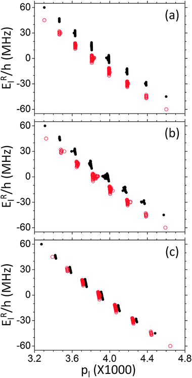 | ||
| Fig. 9 Population vs. energy diagrams at different times, for a homogeneously broadened system composed of seven electrons and a single nucleus with ωn/2π = 15 MHz. This was done using cw MW irradiation for a duration of 0.5 ms (a), 5 ms (b), or 50 ms (c), applied at (ΔωMW − ωe)/2π = −15 MHz. The black dots and red circles correspond to populations of states with σ = ∓1, respectively. All other parameters of the system are given in Table 1. | ||
The examples shown here demonstrate very clearly that the spin temperature concept is an inherent feature of the theoretical model we have been using for the description of the DNP processes. However, up to this point this was only done for a homogeneously broadened EPR line. In the next section we will briefly address the presence of anisotropic g-tensor interactions, leading to an inhomogeneously broadened line.
4. Electrons with an inhomogeneously broadened EPR line
In this section we discuss some aspects related to spin temperature and DNP enhancements in samples where the radicals have an inhomogeneously broadened EPR spectrum. In such systems application of MW irradiation can result in saturation of some of the electrons, leaving others unaffected. To model these conditions, we again use a system with seven electrons, ea with a = 1,…,7, and a single nucleus hyperfine coupled to one of the electrons. However, here the seven electrons have different g-tensor orientations and thus different values of δa. The differences between the frequencies of a pair of electrons are chosen such that they are larger than their dipolar interaction |δa − δb| ≫ |Δab|. In that case the flip–flop terms of the dipolar interactions will generally cause only very small mixing between electronic states. In such a case the eigenstates of the system are almost identical to the product spin states, with some small state mixing due to the pseudo-hyperfine and the dipolar flip–flop interaction terms. The secular part of the dipolar interaction can cause significant frequency shifts, resulting in a spread of the SQ, DQ and ZQ transition frequencies.30 A strong electron–nuclear mixing of states can however occur when states of the type
  and
and  become degenerate, as for two electrons a and b at their CE condition, |δa − δb| ≈ ωn.
4.1 An electron spin system {e7}
At first let us consider a simple system composed of electron spins only, where the effect of the nonsecular part of the dipolar interaction can be neglected, and where the MW irradiation saturates a single electron ec. The state of the system can be described using the populations corresponding to the
  eigenstate, which are in this case equal to the pure electron product states. Since a single electron is saturated by the MW irradiation, it is convenient to redefine the states as
  and
and  , where
  is the total angular momentum of all the non-irradiated electrons, and the α, β superscripts represent the state of the irradiated electron ec. The result of the selective MW saturation of this electron is that
  for all
  and k values. Since all other electrons are unaffected by the MW irradiation, they will retain their thermal equilibrium distribution. The spin system in the rotating frame can therefore be described by the thermal equilibrium electron Zeeman temperature (related to terms in ρΛ which are proportional to
 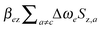 ) and the g-distribution temperature (related to
  ) for all unirradiated electrons, and a single infinite temperature to describe the state of the saturated electron (related to β∞{(Δωe+δc)Sz,c}).
Our small electron spin system resembles the spin system considered by Borghini to describe thermal mixing in systems with an inhomogeneous EPR line.16,34,35 In order to obtain a common temperature for the electrons, Borghini assumed a dipolar driven relaxation mechanism leading to cross relaxations between the electrons. Thus following Borghini we now introduce dipolar relaxation into our seven-electron spin system as it was introduced in eqn (12). When the MW field is sufficiently strong to maintain the saturation condition  , the dipolar relaxation will try to keep the values
  and
and  with Δme = 0 close together (assuming that
  ), while the electron spin–lattice relaxation will try to reach
  . The combination of these three mechanisms can result in a partial saturation of all electrons, which can be described as an increase of the electron Zeeman temperature of the non-irradiated electrons. Thus the dipolar relaxation influences the polarizations of all the (effectively non-irradiated) electrons and their partial saturation is a manifestation of spectral diffusion.
The present model system is of course an over-simplified representation of a real system, where the off-resonance values are not discrete and each MW field has an excitation bandwidth exciting electrons in some frequency range. Then, even when the EPR spectrum is much broader than the dipolar interactions, the dipolar flip–flop terms of coupled electrons with similar off-resonance values are not quenched. However, for broad EPR lines, such as of nitroxides, even for relatively high radical concentrations (e.g. 40 mM) in amorphous solutions most of the electrons with similar off-resonance values will be removed from each other and are therefore only weakly coupled.30 Thus overall only a small fraction of these electrons experience effective interactions that are large. We therefore believe that our electron spin model, despite its simplicity, has some significance for understanding the spin dynamics in real samples.
4.2 An electron spin system coupled to a nucleus {e7–n}
At this stage we can reintroduce the nucleus to the electron system, realizing that it will have a minor effect on the electron populations. Our spin system consists now of seven electrons and a nucleus, where still |δa − δb| ≫ |Δab| for all electrons. In an effort to characterize the main DNP processes present in this system, we will here show some simulated polarization profiles and population–energy diagrams. During these calculations all electrons were coupled to one another with some random interaction coefficients in the range of 0.25–0.75 MHz, and without having a specific structural conformation in mind. An external magnetic field of 3.4 Tesla was chosen and the nucleus was a proton spin, with a Larmor frequency of ωn/2π = 144 MHz. This proton was hyperfine coupled to electron e1 with interaction coefficients of A±1n/2π = 1 MHz and Az,1n = 0. The individual anisotropic Zeeman terms of the electrons were equally spaced, with δa/2π values in the range of ±108 MHz. These values were chosen such that the difference between the off-resonance values of electron e1 and e5 was equal to the proton Larmor frequency, (δ1 − δ5) = ωn. The MW irradiation frequency was varied, exciting one or more of the transitions of the system, namely the SQ transitions of each individual electron and the DQ and ZQ transitions of electron e1. In the system used for the simulations the DQ transitions are located outside of the EPR line, and the ZQ transitions coincide with the SQ spectrum of electron e5. Once again we realize that all of these transitions are split by the secular terms of the electron–electron dipolar interactions.Fig. 10 shows the steady state polarizations of the individual electrons and the nucleus as a function of the frequency of an applied MW field with an intensity of 400 kHz. In (a,c) the dipolar relaxation time is much longer than the electron spin–lattice relaxation time, T1D ≫ T1e, and in (b,d) the dipolar relaxation time is short, namely T1D = 0.1T1e. In all cases the presence of the nucleus has little effect on the steady state electron polarizations, which are plotted in black for electron e1 and in gray for the other six electrons. While for long T1D the individual electrons are saturated without influencing the other electrons, for short T1D all electrons are depopulated when the MW is applied at one of the electron frequencies. This collective polarization depletion is thus the manifestation of spectral diffusion in our system.
 | ||
| Fig. 10 Steady state electron and nuclear polarization as a function of the cw MW irradiation frequency. This was done for an inhomogeneously broadened system composed of seven electrons and a single proton with ωn/2π = 144 MHz (blue line), hyperfine coupled to electron e1 (black line). The polarization of all other electrons is drawn using gray lines. Each electron ej= 1,…,7 has a frequency of ωe/2π+(j − 4) × 36 MHz. In (a) and (b) the dipolar interaction between electrons e1 and e5, which are separated by 144 MHz, was removed, and was reintroduced in (c) and (d). In (a) and (c) the dipolar relaxation is very long, T1D = 10000 s, and in (b) and (d) it is short, T1D = 1 ms, with respect to T1e. The other interaction parameters of this system are: MW power of ω1/2π = 400 kHz; Az,an = 0; A±1n/2π = 1; A±(a≠1)n = 0. The dipolar interaction between each electron pair was given a random value between 0.25 and 0.75 MHz. The other relaxation parameters are the same as in Table 1. | ||
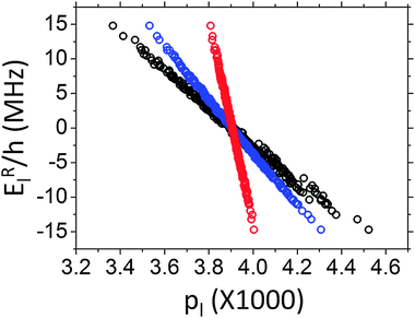
To obtain Fig. 10a and b the dipolar interaction term between electrons e1 and e5 was set to zero. As can be clearly seen, the nuclear polarization is positive when irradiated at the DQ frequency of e1, and negative when irradiated at the ZQ frequency. Some minor enhancement can also be seen when irradiating the SQ transitions of the electrons, but the main polarization mechanism is SE-DNP. The dipolar relaxation does not change the DNP mechanism, but reduces the DNP efficiency due to a depletion of the electron polarization.
For Fig. 10c and d the e1–e5 interaction terms are reintroduced. In this case we observe large nuclear polarization enhancements when the MW is set at the SQ frequencies of e1 and e5, because of the overlap between the SQ and ZQ frequency of e1 and the DQ and SQ frequency of e5, respectively. Thus the CE-DNP mechanism dominates the enhancement profile, when the irradiation is applied within the EPR line. In addition irradiation on the DQ transition of electron e1 results again in enhancements due to the SE mechanism. As before, the dipolar relaxation reduces the steady state enhancements but does not influence the DNP mechanisms. Irradiation on any of the electrons, except e1 and e5, does not result in nuclear polarization and we do not observe any clear signature of a relaxation induced TM-DNP process.
This can also be seen in the steady state population–energy diagrams of the four systems of Fig. 10, as shown in Fig. 11. Here the MW field is applied at the coalescing ZQ and SQ frequencies of e1 and e5. Each symbol in the figure is composed of two populations, corresponding to  , that are equal due to the saturation of the SQ transitions of electron e5. For all four systems we do not observe any process which can be attributed to thermal contact between the electron Zeeman temperature and the g-distribution temperature. In Fig. 11a and c the rotating frame electron Zeeman temperature of all electrons, except e5, stays about equal to βR = Δωe/ωeβL and in Fig. 11b and d this temperature increases. The g-distribution temperature stays close to βL in all cases, because the MW only partially excites the ea≠5 electrons, and because the dipolar relaxation tries to maintain this value for each of the
  manifolds. In all four systems the nucleus gets polarized, and thus the nuclear Zeeman temperature decreases, but this clearly cannot be described as a thermal contact process involving the g-distribution reservoir.
 | ||
| Fig. 11 Steady state population vs. energy diagrams for the inhomogeneously broadeneds systems described in Fig. 10. This was done using MW irradiation with a frequency of (ωMW − ωe)/2π = 36 MHz. The black dots and red circles correspond to states with σ = ∓1, respectively. The parameters used in (a)–(d) are the same as in Fig. 10(a)–(d), respectively. | ||
The fact that the dipolar relaxation does not support the generation of nuclear polarization is not surprising, since the solid state DNP mechanisms require a MW excitation of DQ or ZQ transitions. As mentioned above, the dipolar relaxation does not influence the eigenstates of the system and does not influence the excitation efficiency of the forbidden transitions. In general, relaxation phenomena can of course generate nuclear polarizations when there exists a difference between the electron–nuclear cross relaxation times of the DQ and ZQ transitions, as in the Overhauser effect responsible for liquid-DNP and DNP on conducting solids.1 However, since we did not introduce this type of the relaxation into our model and the electron–electron dipolar relaxation does not involve electron–nuclear cross relaxation mechanisms we do not expect that the dipolar relaxation will contribute to the DNP enhancement.
5. Discussion
In this work we have extended a theoretical model based on the density matrix formalism together with relaxation, previously used to describe the SE-DNP and CE-DNP mechanisms, to investigate TM-DNP. As before, all DNP processes were demonstrated via simulations on small model systems, taking into account simple relaxation mechanisms. The TM-DNP mechanism is commonly formulated in terms of the spin temperature formalism, which describes the relationship between the spin state populations (i.e. the spin density operator) and the energies (i.e. the Hamiltonian) of the system using macroscopic temperature coefficients. Here we have shown that the interaction and relaxation parameters of our model system can be sufficient for the creation of well defined spin temperatures, without a priori assuming their existence. We have interpreted the results using state mixing, effective MW irradiation fields, and spin–lattice relaxation mechanisms. Where possible the results were also described in terms of thermodynamic concepts such as temperature equilibration and heating of spin-baths.Two types of model spin systems were discussed: systems with a homogeneously broadened EPR line, where the electron dipolar interactions strongly mix the electron spin states, such that the MW irradiation and T1e processes are non-electron spin selective; and systems with an inhomogeneously broadened EPR line, where the flip–flop terms of the dipolar interaction are largely quenched, the spin states are hardly mixed, and the MW irradiation and T1e are electron spin selective, even in the presence of electron cross relaxation. Due to computational limitations, our model systems are too small to predict experimental results for systems containing dipolar coupled multi-nuclear networks. However, they did give us some additional insights into the general concept of spin temperature and in particular on the TM phenomena, which are extensively used to interpret DNP experiments.
For the homogeneously broadened electron systems we considered nuclei with Larmor frequencies ωn that were smaller or larger than the EPR line width ΔEPR. In both cases the population distribution of the eigenstates close to steady state during MW irradiation could be described in terms of three spin temperature coefficients, βen, βnz and βdip, in the rotating frame. Starting with different values, strong enough MW irradiation succeeded to equalize the corresponding steady state Ten and Tnz temperatures, while in addition Tnz = Tdip, for ωn < ΔEPR, as expected for TM-DNP. Another property related to TM-DNP which was found in our model was that for ωn < ΔEPR the nuclear enhancement was ωn independent (at the high temperature limit), such that different nuclei had the same Tnz temperature. The results of our simulations indicate that the MW irradiation, in thermodynamic terms, does indeed allow for a heat exchange between different spin baths, resulting in a common temperature. However, it can also result in a significant heating of the system: increasing the MW intensity results in higher steady state temperatures (which can even exceed the lattice temperature) due to off resonance irradiation effects. It was not possible here to derive simple rate equations for the temperature coefficients, predicting their temporal dependence. That this is not possible could be related to the actual DNP mechanism, or to the small size of our system.
The limitation of our calculations for treating many spins becomes more acute when considering inhomogeneously broadened electron spin systems. The interplay between the dipolar broadening and the g-tensor frequency distribution cannot be studied properly, when dealing with only eight spins. Thus we have restricted ourselves to the extreme case where the difference in electron frequency is large enough to enable MW saturation of single electrons, and the dipolar flip–flop terms are significantly quenched to prevent electron state mixing. In this system the DNP enhancements originate solely from the SE and CE mechanisms, even in the presence of dipolar relaxation induced spectral diffusion. It has been argued that such a relaxation mechanism can be very important in the distinction between systems exhibiting TM and CE mechanisms,40 however in our systems, from inspecting population–energy diagrams, we conclude that there exists no TM-like mechanism responsible for the DNP enhancement. Only when the dipolar quenching is significantly reduced and electron state mixing becomes significant, we can expect TM-type of polarization enhancements. Thus our numerical results suggest that for real systems with broad enough EPR lines and not too high radical concentrations the DNP process is dominated by SE and CE processes and not by TM. This is true even in the presence of spectral diffusion originating from electron–electron dipolar relaxation. This seems to be consistent with 1H-DNP experiments on glass-forming solid solutions containing TEMPOL, as shown in ref. 47. The transition between systems which experience significant TM-DNP effects, as discussed in the previous section, and systems which do not is not discussed in this publication and requires further consideration.
As we mentioned, all our discussions did not address the case of multi-nuclear systems. As long as the dipolar interactions between the nuclei are quenched by the hyperfine interactions, their enhancement mechanisms are very similar to the single nuclear enhancement process discussed in this publication. In homogeneous electron systems these nuclei can thus be characterized by a Tnz spin temperature. When the nuclear dipolar interactions become important, the DNP enhancement is mediated by the combined hyperfine and nuclear dipolar flip–flop terms. In such a case different electrons can contribute to the polarization of remote nuclei. This is expected in real samples with high enough electron concentration, for all the DNP mechanisms. How this nuclear spin system will behave under TM-DNP conditions is hard to predict, and we will have to leave this question for future studies.
Acknowledgements
This work was supported by the German-Israeli Project Cooperation of the DFG, through a special allotment by the Ministry of Education and Research (BMBF) of the Federal republic of Germany. Furthermore, this research was made possible in part by the historic generosity of the Harold Perlman Family. S.V. holds the Joseph and Marian Robbins Professorial Chair in Chemistry.References
- Albert Overhauser, Polarization of nuclei in metals, Phys. Rev., 1953, 92(2), 411–415 CrossRef CAS.
- T. Carver and C. Slichter, Polarization of nuclear spins in metals, Phys. Rev., 1953, 92(1), 212–213 CrossRef CAS.
- M. Rosay, J. C. Lansing, K. C. Haddad, W. W. Bachovchin, J. Herzfeld, R. J. Temkin and R. G. Griffin, High-frequency dynamic nuclear polarization in MAS spectra of membrane and soluble proteins, J. Am. Chem. Soc., 2003, 125(45), 13626–136267 CrossRef CAS.
- K. Golman, R. I. T. Zandt, M. Lerche, R. Pehrson and J. H. Ardenkjaer-Larsen, Metabolic imaging by hyperpolarized 13C magnetic resonance imaging for in vivo tumor diagnosis, Cancer Res., 2006, 66(22), 10855–10860 CrossRef CAS.
- K. Golman, R. I. T. Zandt and M. Thaning, Real-time metabolic imaging, Proc. Natl. Acad. Sci. U. S. A., 2006, 103(30), 11270–11275 CrossRef CAS.
- A. P. Chen, M. J. Albers, C. H. Cunningham, S. J. Kohler, Y.-F. Yen, R. E. Hurd, J. Tropp, R. Bok, J. M. Pauly, S. J. Nelson, J. Kurhanewicz and D. B. Vigneron, Hyperpolarized C-13 spectroscopic imaging of the TRAMP mouse at 3T-initial experience, Magn. Reson. Med. Official Journal of the Society of Magnetic Resonance in Medicine, 2007, 58(6), 1099–1106 CAS.
- F. A. Gallagher, M. I. Kettunen, S. E. Day, D.-E. Hu, J. H. Ardenkjaer-Larsen, R. Zandt, P. R. Jensen, M. Karlsson, K. Golman, M. H. Lerche and K. M. Brindle, Magnetic resonance imaging of pH in vivo using hyperpolarized 13C-labelled bicarbonate, Nature, 2008, 453(7197), 940–943 CrossRef CAS.
- F. A. Gallagher, M. I. Kettunen, D.-E. Hu, P. R. Jensen, R. I. T. Zandt, M. Karlsson, A. Gisselsson, S. K. Nelson, T. H. Witney, S. E. Bohndiek, G. Hansson, T. Peitersen, M. H. Lerche and K. M. Brindle, Production of hyperpolarized [1,4-13C2] malate from [1,4-13C2] fumarate is a marker of cell necrosis and treatment response in tumors, Proc. Natl. Acad. Sci. U. S. A., 2009, 106(47), 19801–19806 CAS.
- F. A. Gallagher, M. I. Kettunen and K. M. Brindle, Biomedical applications of hyperpolarized 13C magnetic resonance imaging, Prog. Nucl. Magn. Reson. Spectrosc., 2009, 55(4), 285–295 CrossRef CAS.
- V. Bajaj, M. L. Mak-Jurkauskas, M. Belenky, J. Herzfeld and R. G. Griffin, Functional and shunt states of bacteriorhodopsin resolved by 250 GHz dynamic nuclear polarization-enhanced solid-state NMR, Proc. Natl. Acad. Sci. U. S. A., 2009, 106(23), 9244–9249 CrossRef CAS.
- D. M. Wilson, K. R. Keshari, P. E. Z. Larson, A. P. Chen, S. Hu, M. Van Criekinge, R. Bok, S. J. Nelson, J. M. Macdonald, D. B. Vigneron and J. Kurhanewicz, Multi-compound polarization by DNP allows simultaneous assessment of multiple enzymatic activities in vivo, J. Magn. Reson., 2010, 205(1), 141–147 CrossRef CAS.
- J. H. Ardenkjaer-Larsen, B. Fridlund, A. Gram, G. Hansson, L. H. Hansson, M. H. Lerche, R. Servin, M. Thaning and K. Golman, Increase in signal-to-noise ratio of >10000 times in liquid-state NMR, Proc. Natl. Acad. Sci. U. S. A., 2003, 100(18), 10158–10163 CrossRef CAS.
- R. A. Wind, M. J. Duijvestijn, C. van der Lugt, A. Manenschijn and J. Vriend, Applications of dynamic nuclear polarization in 13C NMR in solids, Prog. Nuc. Mag. Res. Sp., 1985, 17, 33–67 CrossRef CAS.
- L. R. Becerra, G. J. Gerfen, R. J. Temkin, D. J. Singel and R. G. Griffin, Dynamic nuclear polarization with a cyclotron resonance maser at 5 T, Phys. Rev. Lett., 1993, 71(21), 3561–3564 CrossRef CAS.
- G. J. Gerfen, L. R. Becerra, D. a. Hall, R. G. Griffin, R. J. Temkin and D. J. Singel, High frequency (140 GHz) dynamic nuclear polarization: polarization transfer to a solute in frozen aqueous solution, J. Chem. Phys., 1995, 102(24), 9494 CrossRef CAS.
- A. Abragam and M. Goldman, Principles of dynamic nuclear polarisation, Rep. Prog. Phys., 1978, 41(3), 395–467 CrossRef CAS.
- N. Bloembergen, On the interaction of nuclear spins in a crystalline lattice, Physica, 1949, 15(3–4), 386–426 CrossRef CAS.
- A. G. Redfield, Nuclear magnetic resonance saturation and rotary saturation in solids, Phys. Rev., 1955, 98(6), 1787–1809 CrossRef CAS.
- B. N. Provotorov, Magnetic resonance saturation in crystals, Sov. Phys. – JETP, 1962, 14(5), 1126–1131 Search PubMed.
- C. Jeffries, Polarization of nuclei by resonance saturation in paramagnetic crystals, Phys. Rev., 1957, 106(1), 164–165 CrossRef CAS.
- A. Abragam and W. G. Proctor, Une nouvelle methode de polarisation dynamique des noyaux atomiques dans les solides, C. R. Hebd. Seances Acad. Sci., 1958, 246, 2253–2256 CAS.
- A. V. Kessenikh, V. I. Lushchikov, A. A. Manenkov and Y. V. Taran, Sov. Phys. – Solid State, 1963, 5, 321–329 Search PubMed.
- A. V. Kessenikh, V. I. Luschikov and A. A. Manenkov, Sov. Phys. – Solid State, 1963, 5, 835–837 Search PubMed.
- A. V. Kessenikh, A. A. Manenkov and G. I. Pyatnitskii, Sov. Phys. – Solid State, 1964, 6, 641–643 Search PubMed.
- C. Hwang and D. Hill, Phenomenological model for the new effect in dynamic polarization, Phys. Rev. Lett., 1967, 19(18), 1011–1014 CrossRef CAS.
- K.-N. Hu, G. T. Debelouchina, A. Smith and R. G. Griffin, Quantum mechanical theory of dynamic nuclear polarization in solid dielectrics, J. Chem. Phys., 2011, 134(12), 125105 CrossRef.
- Y. Hovav, A. Feintuch and S. Vega, Theoretical aspects of dynamic nuclear polarization in the solid state - the solid effect, J. Magn. Reson., 2010, 207(2), 176–89 CrossRef CAS.
- Y. Hovav, A. Feintuch and S. Vega, Dynamic nuclear polarization assisted spin diffusion for the solid effect case, J. Chem. Phys., 2011, 134(7), 074509 CrossRef.
- Y. Hovav, A. Feintuch and S. Vega, Theoretical aspects of dynamic nuclear polarization in the solid state - the cross effect, J. Magn. Reson., 2012, 214(1), 29–41 CrossRef CAS.
- Y. Hovav, O. Levinkron, A. Feintuch and S. Vega, Theoretical aspects of dynamic nuclear polarization in the solid state: the influence of high radical concentrations on the solid effect and cross effect mechanisms, Appl. Magn. Reson., 2012, 43(1–2), 21–41 CrossRef CAS.
- A. Karabanov, I. Kuprov, G. T. P. Charnock, A. van der Drift, L. J. Edwards and W. Köckenberger, On the accuracy of the state space restriction approximation for spin dynamics simulations, J. Chem. Phys., 2011, 135(8), 084106 CrossRef.
- A. Karabanov, A. van der Drift, L. J. Edwards, I. Kuprov and W. Kockenberger, Quantum mechanical simulation of solid effect dynamic nuclear polarisation using Krylov–Bogolyubov time averaging and a restricted state-space, Phys. Chem. Chem. Phys., 2012, 14(8), 2658–2668 RSC.
- I. Solomon, Magnetic Resonance and Relaxation, North-Holland, Amsterdam, 1963 Search PubMed.
- A. Abragam and M. Borghini, Dynamic polarization of nuclear targets, in Progress in Low Temperature Physics, North-Holland Publishing Company, Amsterdam, 1964, pp. 384–449 Search PubMed.
- M. Borghini, Spin-temperature model of nuclear dynamic polarization using free radicals, Phys. Rev. Lett., 1968, 20(9), 419–421 CrossRef CAS.
- L. L. Buishvili, Sov. Phys. – JETP, 1966, 22, 1277 Search PubMed.
- M. Goldman, Spin temperature and nuclear magnetic resonance in solids, Clarendon Press, Oxford, 1970 Search PubMed.
- W. Boer, Dynamic orientation of nuclei at low temperatures, J. Low Temp. Phys., 1976, 22(1–2), 185–212 CrossRef.
- S. Goertz, The dynamic nuclear polarization process, Nucl. Instrum. Methods Phys. Res., Sect. A, 2004, 526(1–2), 28–42 CrossRef CAS.
- V. A. Atsarkin and A. V. Kessenikh, Dynamic nuclear polarization in solids: the birth and development of the many-particle concept, Appl. Magn. Reson., 2012, 43(1–2), 7–19 CrossRef.
- S. Jannin, A. Comment, F. Kurdzesau, J. Konter, P. Hautle, B. van den Brandt and J. J. van der Klink, A 140 GHz prepolarizer for dissolution dynamic nuclear polarization, J. Chem. Phys., 2008, 128(24), 241102 CrossRef CAS.
- S. Jannin, A. Comment and J. J. van der Klink, Dynamic nuclear polarization by thermal mixing under partial saturation, Appl. Magn. Reson., 2012, 43(1–2), 59–68 CrossRef CAS.
- A. Schweiger and G. Jeschke, Principles of pulse electron paramagnetic resonance, Oxford University edition, 2001 Search PubMed.
- A. Karabanov, G. Kwiatkowski and W. Kockenberger, Quantum mechanical simulation of cross effect DNP using Krylov–Bogolyubov averaging, Appl. Magn. Reson., 2012, 43(1–2), 43–58 CrossRef CAS.
- J. van Houten, W. T. h. Wenckebach and N. J. Poulis, A study of the thermal contact between the nuclear Zeeman system and the electron dipole–dipole interaction system, Physica B+C, 1977, 92(2), 210–220 CrossRef.
- S. Stoll, B. Epel, S. Vega and D. Goldfarb, Ligand protons in a frozen solution of copper histidine relax via a T1e-driven three-spin mechanism, J. Chem. Phys., 2007, 127(16), 164511 CrossRef CAS.
- D. Shimon, Y. Hovav, A. Feintuch, D. Goldfarb and S. Vega, Dynamic nuclear polarization in the solid state: a transition between the cross effect and the solid effect, Phys. Chem. Chem. Phys., 2012, 14(16), 5729–5743 RSC.
| This journal is © the Owner Societies 2013 |