Quantitative analysis of atmospheric volatile organic pollutants by thermal desorption gas chromatography mass spectrometry

Abstract

An analytical method has been developed and validated for analyzing 48 volatile organic compounds (VOCs) that were found to be present in substantial quantities in the atmosphere in Singapore. Air samples were collected by active sampling using Tenax/Carbopack X multisorbent tubes and were evaluated by Thermal Desorption Gas Chromatography Mass Spectrometry (TD-GCMS). Experiments conducted using standards demonstrated excellent repeatability with relative standard deviation (%RSD) values lesser than 10%, good linearity with R² values of at least 0.99 for a wide range of concentrations between 0.02 and 500 ng, breakthrough values 5% or lower, tube desorption efficiencies close to 100% and good recoveries between 61% and 120%. Sampling volumes and flow rates were tested and selected by evaluating the performance of the multisorbent tubes. 30 mL min⁻¹ was selected as the optimal flow rate for different sampling volumes depending on the individual compound's breakthrough value and reproducibility during air sampling. Most of the target analytes exhibited acceptable breakthrough of 5% or less, reproducibility within 20% deviation and method detection limits below 500 ppbv. Criteria established by the United States Environmental Protection Agency (USEPA) for sorbent tube sampling (EPA TO-17) were met for most compounds of interest.

---

Introduction

The analysis of VOCs in ambient air is becoming increasingly important due to continuous global industrialization. Localised levels of certain VOCs present in the atmosphere could become potentially harmful to living organisms. The environmental and health effects of VOCs were well-established in several previous studies.^1–4 Some of these organic pollutants play important roles in stratospheric ozone depletion, the greenhouse effect and photochemical smog. Short term exposure to VOCs can induce irritation of mucous membranes, nausea, increase the risk of asthma and affect the nervous, immune and reproductive systems.^5–7 Long term exposure to some compounds can lead to mutagenic and carcinogenic effects.⁸

Despite of the possible environmental and health risks, the monitoring of atmospheric VOCs by regulatory boards are not complete. The regulation of outdoor VOCs by several environmental agencies such as the USEPA and the European Environment Agency (EEA) focuses mainly on non-methane VOCs (NMVOCs) that contribute to the production of tropospheric ozone.^9,10 A wider range of VOCs are usually analysed for indoor emissions.^9,11,12 6 major atmospheric contaminants namely: carbon monoxide, lead, oxides of nitrogen, ozone, particulate matter <10 μm and sulfur dioxide are used for monitoring the quality of ambient air.^13–15 The inclusion of several other VOCs might eventually become essential.

Several procedures have been established for monitoring air quality. Solvent extraction coupled with Gas Chromatography Mass Spectrometry (GCMS) is the conventional technique used for evaluating VOCs in the atmosphere.¹⁶ It involves trapping VOCs from the air using activated charcoal, followed by a desorbing solvent, usually carbon disulfide, to extract compounds retained on the surface of the charcoal sorbent which are analysed by GCMS.^17–19 The main disadvantage of this method is that it has comparatively higher detection limits than other VOC analytical techniques.^16,20 The desorbing solvent required to extract the compounds from the charcoal is highly toxic and inevitably dilutes the sample.^19–21 In addition, polar and reactive analytes from the charcoal sorbent cannot desorb efficiently in polar and aqueous environments.^22–24 Low desorption efficiencies of polar and reactive VOCs are related to the strength of several binding interactions, permanent adsorptions and catalytic conversions of the target species into different products.¹⁶

Solvent-free techniques such as sorbent-based sampling and canister-based sampling, both coupled with TD-GCMS for analysis, can also be used for quantifying atmospheric VOCs. Sorbent-based sampling methods use tubes containing solid sorbent materials to retain organic pollutants present in the air.^25–29 The canister-based sampling method employs clean stainless steel canisters for pumping and collecting air samples.^30,31 Sorbent tubes are heated to high temperatures to desorb analytes. A flow of inert gas is used to extract and transfer these compounds into a cold trap.³² The trap preconcentrates and focuses all the compounds from the tube, before inverting the flow of inert gas and heating itself to high temperature.³³ Target compounds are injected into the GC column for further separation and analysis. For canisters, an aliquot of air is preconcentrated into the cold trap directly.³⁴ The trap desorbs at high temperature and together with a flow of inert gas, injects the VOCs into the GCMS. The main advantage of using TD-GCMS is that the method is highly compatible for a wide range of VOCs of varying polarities. Sorbent tubes are reusable for a long period of time, and are portable and easy to store.^21,35 In addition, solvent is not required for the extraction step.²⁰

In this study, 48 VOCs present in ambient air from the industrialized region of Singapore were identified by active sorbent-based sampling and an analytical method was developed for quantifying these compounds using TD-GCMS.

Experimental

Chemicals and standard solutions

Neat chemicals were purchased as VOC reference standards from Sigma-Aldrich (St Louis, USA), Merck (Hohenbrunn, Germany), Alfa Aesar (Heysham, Lancaster, UK) and Fluka (Buchs, Switzerland) with purity not less than 97%, except for the following compounds: 1,2,3-trimethylbenzene (93.9%) from Fluka and methacrolein (95%) from Sigma-Aldrich.

Stock solutions of individual compounds were prepared by extracting 1 mL of standards into 5 mL volumetric flasks, topped with methanol (Tedia, Fairfield, USA) and homogenized by shaking. The individual stock solutions were diluted to 50 g L⁻¹ solutions. A 500 ng μL⁻¹ standard mixture was prepared next by extracting 500 μL of the 50 g L⁻¹ individual standard solutions into the same 50 mL volumetric flask, topped with methanol and homogenized by shaking. Experiments carried out on the mixture have shown that it is stable for at least a week when stored at 4 °C in darkness. The calibration mixture was further diluted to VOC standards of varying concentrations ranging from 0.02 to 500 ng μL⁻¹. All VOC standards were newly prepared before an instrumental run from the 500 ng μL⁻¹ mixture.

Sorbent tubes

For this study, sorbent tubes (3.5 in. (89 mm) × 0.25 in. (6.4 mm) o.d.) prepacked with 200 mg of Tenax and 100 mg of Carbopack X (Markes International Limited, Llantrisant, U.K.) were used for retaining target analytes from standards and air samples. When compared to single sorbent materials, multisorbent tubes are more capable of retaining and desorbing a wider spectrum of analytes with varying polarities and boiling points. Tenax is a weak strength sorbent that is selective for aromatic compounds, non-polar compounds with boiling point above 100 °C and polar compounds with boiling points below 150 °C. Carbopack X has sorbent strength between medium to strong and is specific for analytes that are more volatile, with boiling points between 50 °C and 150 °C. In addition, both materials are hydrophobic to prevent the effects of humidity on adsorption and desorption. Sorbents were packed in order of increasing sorbent strength, each material separated by quartz wool and wire gauze. New sorbent tubes were conditioned at 320 °C for 2 hours, followed by 335 °C for 30 minutes for the first time before usage. Subsequent conditionings after usage were carried out at 320 °C for 30 minutes. All conditionings were conducted under helium flow of 70 mL min⁻¹.

For the preparation of calibration standards, 1 μL of VOC standards was injected into individual multisorbent tubes using a GC syringe via a calibration loading ring. The solution in the GC syringe was introduced into the sorbent tube with pure nitrogen gas (99.999%) flowing in the direction of the injection. The GC syringe needle was kept within the loading ring for a short interval of 20 to 30 seconds to achieve complete evaporation of target analytes. The nitrogen gas aids the retention of the VOC onto the sorbent beds and removes the methanol solvent out of the tube.

Instrumentation

A UNITY series 2 (Markes International Limited, Llantrisant, U.K.) was used for the thermal desorption process and an Ultra autosampler (Markes International Limited, Llantrisant, U.K.) was utilised for automated analysis of multiple sorbent tubes. Two stages were involved during the thermal desorption process: primary desorption followed by secondary desorption. In the primary desorption stage (also known as tube desorption), VOCs were extracted from the sorbent tube by simultaneously heating the tube to 280 °C for 10 minutes and introducing a stream of high purity helium (99.999%) at 45 mL min⁻¹ through the tube. All compounds released from the multisorbent tube were transferred and preconcentrated onto a hydrophobic Tenax trap cooled at −10 °C using splitless mode. During secondary desorption (also known as trap desorption), the inversion of helium flowing through the cold trap took place. At the same time, the trap was heated to 300 °C at the maximum temperature ramp rate for 7 minutes to carry the desorbed VOCs into the GC column (Agilent J & W 122-1564 260 °C 60 m × 250 μm × 1.4 μm DB-VRX 1219.45766) where the separation of VOCs was carried out, using a split flow of 6 mL min⁻¹. As a result, a split ratio of 5 : 1 was attained. The temperature gradient of the GC oven was programmed at 30 °C for 12 minutes, increased to 60 °C at a rate of 30 °C min⁻¹, followed by an increase to 124 °C at a rate of 40 °C min⁻¹. The oven was held at 200 °C for another 2 minutes. High purity helium (99.999%) was used as the carrier gas for GC analysis and a constant flow of 1.5 mL min⁻¹ was applied. The GCMS interface was kept constant at 250 °C. The mass spectrometer acquired data in scan mode at a mass range from 35–300 amu. The ion source (70 eV electron impact) temperature was set at 230 °C and the quadrupole was held at 150 °C. Target analytes were qualitatively identified by comparing the retention time, relative abundance of the qualifier ions and quantifier ion to those of VOC standards. Quantification of target compounds from samples collected was performed using an external calibration method of the quantifier ion, using the VOCs standards of different concentrations. A summary of the quantifier ion, qualifier ions Q1 and Q2 for all the compounds of interest are shown in Table 1.

Table 1 Target analytes in chromatographic elution order, their quantifier ions, qualifier ions and summary of method validation data for standards^a,b

VOC reference no.	Target analytes	Quantifier ion	Qualifier ions		t R (min)	%RSD (n = 6)	R ^2	Breakthrough (%)	LOD (ng)	LOQ (ng)	Tube desorption efficiency (%)	Accy (%)
			Q1	Q2
a Retention times (tR), repeatability, expressed as percentage relative standard deviation (%RSD) for the analysis of 100 ng of standards (n = 6), linearity expressed as linear regression coefficient (R^2), breakthrough (% VOC present in the back tube), limit of detection (LOD), limit of quantification (LOQ), tube desorption efficiency (%) and accuracy (Accy%). %RSD rounded to nearest whole number. b Under the breakthrough column, <d.l. indicates that the VOC present in the back tube was less than the limit of detection, hence no accurate calculation could be performed to obtain a numerical value; 0.00 stands for VOC absent in the back tube. The values in the bracket next to the qualifier ions: Q1 and Q2 are the percentage relative abundance of the ions with respect to the base ion.
1	Isopropyl alcohol	45	43 (17)	59 (5)	8.21	2	0.9971	1.14	0.01	0.04	100	61
2	Ethyl ether	59	45 (65)	73 (12)	8.80	3	0.9988	0.00	0.38	1.28	100	71
3	2-Methyl-1,3-butadiene	67	68 (69)	53 (54)	9.11	4	0.9986	0.00	0.08	0.27	100	80
4	Dichloromethane	84	49 (90)	86 (65)	10.27	2	0.9983	2.13	0.03	0.09	99.7	72
5	2-Methylpentane	71	43 (100)	42 (53)	13.01	3	0.9986	0.00	0.16	0.55	100	82
6	Methacrolein	70	41 (84)	39 (73)	13.25	3	0.9963	0.00	0.05	0.16	99.7	66
7	3-Methylpentane	57	56 (87)	41 (52)	13.63	3	0.9981	0.34	0.02	0.07	99.9	82
8	Hexane	57	41 (60)	43 (51)	14.21	3	0.9991	0.53	0.04	0.12	99.5	64
9	2-Butanone	72	43 (100)	57 (8)	14.26	2	0.9981	0.67	0.01	0.04	99.6	66
10	Trichloromethane	83	85 (67)	47 (17)	14.70	2	0.9993	0.65	0.01	0.05	99.8	63
11	Ethyl acetate	43	61 (19)	70 (15)	14.79	2	0.9994	<d.l.	0.04	0.13	99.8	99
12	Methylcyclopentane	56	69 (48)	41 (42)	15.05	3	0.9994	0.26	0.01	0.04	99.7	86
13	Cyclohexane	84	56 (95)	41 (43)	15.98	2	0.9995	0.00	0.05	0.16	100	81
14	Benzene	78	77 (22)	51 (12)	16.16	2	0.9986	0.00	1.03	1.68	98.9	84
15	Heptane	71	43 (100)	57 (64)	16.89	5	0.9980	0.00	0.17	0.58	100	84
16	Trichloroethylene	130	132 (97)	134 (31)	16.97	2	0.9989	0.00	0.01	0.02	100	73
17	Methyl methacrylate	69	41 (85)	39 (46)	17.27	2	0.9971	0.00	0.08	0.26	99.7	67
18	Methyl cyclohexane	83	55 (61)	98 (46)	17.58	2	0.9984	0.00	0.04	0.14	100	81
19	Methyl isobutyl ketone	43	58 (48)	85 (25)	17.95	1	0.9990	<d.l.	0.07	0.22	99.8	62
20	Pyridine	79	52 (47)	51 (21)	18.10	5	0.9971	0.00	0.41	1.38	99.9	74
21	2-Methylheptane	57	43 (78)	70 (26)	18.37	2	0.9998	0.00	0.06	0.21	99.9	86
22	Toluene	91	92 (64)	65 (10)	18.70	5	0.9965	1.15	0.09	0.16	99.7	91
23	1-Octene	55	41 (77)	70 (90)	18.88	1	0.9996	<d.l.	0.05	0.17	100	70
24	Octane	43	85 (71)	57 (49)	19.04	1	0.9982	0.00	0.06	0.19	99.9	89
25	Hexanal	56	57 (71)	72 (33)	19.14	2	0.9976	0.40	0.05	0.15	99.7	82
26	Tetrachloroethylene	166	164 (77)	129 (65)	19.58	2	0.9985	0.00	0.01	0.03	100	71
27	Furfural	96	95 (91)	39 (33)	19.95	4	0.9963	0.00	0.32	1.07	99.5	70
28	Ethylbenzene	91	106 (38)	77 (8)	20.63	4	0.9998	0.20	0.01	0.02	99.8	82
29,30	m,p-Xylene	91	106 (56)	77 (12)	20.86	1	0.9947	<d.l.	0.12	0.21	99.8	78
31	Nonane	57	43 (91)	85 (48)	21.00	1	0.9998	0.07	0.07	0.23	99.9	79
32	Heptanal	70	55 (66)	57 (55)	21.16	3	0.9951	1.05	0.05	0.15	99.7	55
33	Styrene	104	103 (46)	78 (37)	21.29	3	0.9985	0.75	0.01	0.02	99.8	75
34	o-Xylene	91	106 (54)	105 (21)	21.39	2	0.9991	0.46	0.03	0.06	99.8	83
35	Phenol	94	66 (24)	65 (20)	22.38	2	0.9925	1.36	1.31	2.24	92.1	88
36	1-Ethyl-3-methylbenzene	105	120 (42)	91 (14)	22.60	1	0.9917	<d.l.	0.02	0.06	99.8	108
37	1-Ethyl-4-methylbenzene	105	120 (39)	91 (12)	22.68	2	0.9972	0.00	0.02	0.06	99.9	111
38	Benzaldehyde	105	106 (97)	77 (87)	22.74	4	0.9909	1.55	0.65	1.25	98.9	88
39	1,3,5-Trimethylbenzene	105	120 (62)	91 (11)	22.85	7	0.9994	0.28	0.01	0.04	99.8	65
40	Decane	57	43 (74)	71 (45)	22.90	1	0.9996	<d.l.	0.04	0.13	99.9	104
41	1-Ethyl-2-methylbenzene	105	120 (42)	91 (13)	23.05	2	0.9941	<d.l.	0.03	0.10	99.8	87
42	Octanal	41	43 (94)	57 (94)	23.13	2	0.9993	0.00	0.08	0.27	99.6	74
43	Benzonitrile	103	76 (32)	50 (10)	23.18	2	0.9983	0.00	0.05	0.16	99.3	113
44	1,2,4-Trimethylbenzene	105	120 (59)	91 (11)	23.41	1	0.9996	0.08	0.02	0.07	99.7	90
45	1,2,3-Trimethylbenzene	105	120 (51)	91 (10)	24.03	1	0.9999	<d.l.	0.03	0.09	99.8	92
46	Acetophenone	105	77 (66)	120 (27)	24.82	4	0.9973	0.96	0.54	0.97	98.8	113
47	Nonanal	57	41 (70)	70 (40)	25.03	6	0.9967	0.46	0.05	0.18	99.5	86
48	Decanal	57	41 (81)	70 (58)	27.03	5	0.9943	1.02	0.07	0.25	99.0	102

---

Results and discussion

Method validation

Validation was carried out by inspecting the following characteristics of the optimized parameters of the TD-GCMS method for VOC analysis: selectivity, precision, linearity, breakthrough, sensitivity, tube desorption efficiency and accuracy.

The GC column and the optimised oven temperature programme are highly selective for all compounds of interest. Excellent chromatographic separation for most target VOCs were observed (Table 1 and Fig. 1). 37 compounds have total ion current (TIC) signals with resolution values of 1.5 and above. 10 compounds had TIC signals with resolutions between 0.745 and 1.33, but could still be quantitatively determined by selecting a characteristic ion absent in the compound that was eluting together with itself, as the quantifier ion (Table 1). Only 1 co-elution was observed from p-xylene and m-xylene, which have to be quantified together as both compounds share the same retention time and mass spectra.

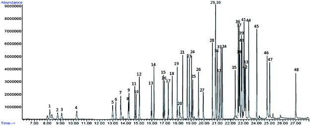Fig. 1 Total ion current chromatogram for 50 ng standard mixture. Corresponding VOC reference numbers are listed in Table 1.

Precision was investigated by analyzing six tubes (n = 6) loaded with the same amount of standard solution. 100 ng of standard solution was injected into each tube. All compounds of interest exhibited excellent repeatability, each having a %RSD value of less than 10% (Table 1). This complies with EPA TO-17 performance guidelines, which require volatile organic analytes to have %RSD values 25% and below.^34,36

The calibration curve of VOC standards was established by plotting the integrated area of response signals as a function of analyte concentration, and the linear relationship between the two functions was investigated.³⁷ This is to determine the range of concentrations over which the analytical method could be applied.³⁷ The linearity of the regression line is defined by the linear regression coefficient (also known as R²).³⁷ The linearity of the multi-point calibration curve was evaluated by analyzing varying amounts of target VOCs between 0.02 ng and 500 ng. All calibration curves plotted for the compounds of interest have good linearity, with R² values bigger than 0.99, for signal to noise ratios ≥10 (Table 1). The limit of quantification (LOQ) of the compounds was taken to be the lowest calibration level. Thus, the R² in Table 1 for each compound is between the LOQ to 500 ng.

Breakthrough is defined as the percentage of VOC mass found in the back sorbent tube when two of such tubes are connected in series. This is investigated to understand the retention capacity of the selected sorbent material chosen for air monitoring. It is important to know if the sorbent materials are durable for retaining high amounts of analytes, without leakages through the sorbent tube. Although breakthrough volumes are available for some analytes on different sorbents, it is important to determine the breakthrough under the present sampling conditions (humidity and temperature) where multisorbents are used. Two types of breakthrough were investigated in this study: (i) during the injection of VOC standards when a flow of carrier gas is used to aid the retention of the sorbent tube (Table 1), and (ii) during sampling when using calibrated air pumps (Tables 2 and 3). The latter will be discussed under the performance evaluation of sorbent tubes section. Breakthrough during the injection of standards was carried out by connecting two Tenax TA/Carbopack X tubes in series. A flow of 99.999% nitrogen gas was introduced into the connected tubes at 100 mL min⁻¹ for 5 minutes. Simultaneously, a 1 μL aliquot of the 500 ng μL⁻¹ standard solution was injected into the inlet end of the first tube. Both tubes were analysed and the response area of target compounds were quantified using the calibration curve constructed by varying concentrations between 0.02 ng and 500 ng. Breakthrough values for each analyte was calculated as a percentage of the mass of VOC analyte found in the back tube to the total mass of VOC present in both tubes.³⁴ All compounds of interest exhibited excellent breakthrough values below 5% during the loading of VOC standards (Table 1). This shows that there is minimal analytes leaking from the front sorbent tube during the preparation of standards for a flow of nitrogen gas at 100 mL min⁻¹.

Table 2 Summary of breakthrough values (%) for selected compounds obtained at varying flow rates (30 mL min⁻¹, 50 mL min⁻¹ and 70 mL min⁻¹) for sampling volumes of 1 L, 5 L and 10 L^a,b

Target analytes	1 Litre			5 Litres			10 Litres
	30 mL min^−1	50 mL min^−1	70 mL min^−1	30 mL min^−1	50 mL min^−1	70 mL min^−1	30 mL min^−1	50 mL min^−1	70 mL min^−1
a Breakthrough (% VOC present in the back tube) at sampling volumes of 1 L, 5 L and 10 L of air at 30 mL min^−1, 50 mL min^−1 and 70 mL min^−1. b n.d. stands for not detected in both tubes; 0.00 stands for VOC absent in the back tube.
Isopropyl alcohol	0.00	0.00	0.00	2.52	4.17	6.03	8.83	10.41	16.10
Ethyl ether	0.00	0.00	0.00	0.00	0.00	26.69	0.00	0.00	25.42
Dichloromethane	9.39	17.90	23.06	41.24	59.71	19.12	38.77	38.26	63.14
Pyridine	n.d.	n.d.	n.d.	n.d.	n.d.	n.d.	n.d.	n.d.	n.d.
Nonanal	0.00	0.00	0.00	0.00	0.00	7.15	13.60	5.35	7.49
Decanal	0.00	0.00	0.00	0.00	n.d.	0.00	7.34	3.79	6.87

---

Table 3 Summary of sorbent tube performance in sampling^a,b

VOC reference no.	Target analytes	Breakthrough at 5 L (%)	%RSD (n = 2)	MDL (μg m^−3)	MQL (μg m^−3)
a Selected sampling volume (L), breakthrough (% VOC present in the back tube), reproducibility expressed as percentage relative standard deviation (%RSD) during sampling using calibrated pumps (n = 2), method detection limit (μg m^−3) and method quantification limit (μg m^−3). %RSD rounded to nearest whole number. b All data are for a sampling flow rate of 30 mL min^−1. Under the breakthrough column, <d.l. and <q.l. indicate that the VOC present in the back tube was less than the limit of detection or limit of quantification, respectively, hence no accurate calculation could be performed to obtain a numerical value; n.d. stands for not detected in both tubes; 0.00 stands for VOC absent in the back tube.
1	Isopropyl alcohol	2.52	1	0.002	0.008
2	Ethyl ether	0.00	5	0.08	0.26
3	2-Methyl-1,3-butadiene	0.00	14	0.02	0.05
4	Dichloromethane	41.24	6	0.006	0.02
5	2-Methylpentane	0.00	3	0.03	0.11
6	Methacrolein	0.00	7	0.01	0.03
7	3-Methylpentane	0.00	5	0.004	0.01
8	Hexane	0.26	1	0.008	0.02
9	2-Butanone	0.00	15	0.002	0.008
10	Trichloromethane	0.00	2	0.002	0.01
11	Ethyl acetate	0.00	18	0.008	0.03
12	Methylcyclopentane	0.00	2	0.002	0.008
13	Cyclohexane	0.00	3	0.01	0.03
14	Benzene	<d.l.	3	0.21	0.34
15	Heptane	0.00	6	0.03	0.12
16	Trichloroethylene	0.00	9	0.002	0.004
17	Methyl methacrylate	0.00	1	0.02	0.05
18	Methyl cyclohexane	0.00	0	0.008	0.03
19	Methyl isobutyl ketone	0.00	3	0.01	0.04
20	Pyridine	n.d.	n.d	n.d.	n.d.
21	2-Methylheptane	0.00	7	0.01	0.04
22	Toluene	0.18	7	0.02	0.03
23	1-Octene	0.00	5	0.01	0.03
24	Octane	0.00	4	0.01	0.04
25	Hexanal	0.00	3	0.01	0.03
26	Tetrachloroethylene	0.00	3	0.002	0.006
27	Furfural	0.00	7	0.06	0.21
28	Ethylbenzene	0.12	3	0.002	0.004
29,30	m,p-Xylene	<d.l.	6	0.02	0.04
31	Nonane	0.00	9	0.01	0.05
32	Heptanal	0.00	18	0.01	0.03
33	Styrene	0.00	0	0.002	0.004
34	o-Xylene	<q.l.	2	0.006	0.01
35	Phenol	<d.l.	0	0.26	0.45
36	1-Ethyl-3-methylbenzene	<q.l.	4	0.004	0.01
37	1-Ethyl-4-methylbenzene	0.00	11	0.004	0.01
38	Benzaldehyde	<d.l.	6	0.13	0.25
39	1,3,5-Trimethylbenzene	0.00	8	0.002	0.008
40	Decane	1.26	9	0.008	0.03
41	1-Ethyl-2-methylbenzene	<d.l.	7	0.006	0.02
42	Octanal	0.00	6	0.02	0.05
43	Benzonitrile	<q.l.	8	0.01	0.03
44	1,2,4-Trimethylbenzene	1.21	8	0.004	0.01
45	1,2,3-Trimethylbenzene	<d.l.	5	0.006	0.02
46	Acetophenone	<d.l.	5	0.11	0.19
47	Nonanal	0.00	0	0.01	0.04
48	Decanal	0.00	18	0.01	0.05

---

Sensitivity of the instrument was validated by evaluating two parameters: limit of detection (LOD) and limit of quantification (LOQ). LOD of a target VOC analyte is the minimum amount of analyte present in a sample that can be detected but not inevitably quantified as an accurate value.³⁷ LOD of a target VOC analyte is the minimum amount of analyte found in a sample that can be quantitatively established with suitable precision and accuracy.³⁷ The LOD and LOQ values were determined using two different methods. For target analytes that were absent from the blanks, LOD is the concentration that gives a signal-to-noise ratio of 3, whereas LOQ is the concentration that gives a signal-to-noise ratio of 10.^34,37,38 Signal-to-noise ratios were obtained by comparing measured signals from samples with known low concentrations of analyte with those of blank samples and determining the minimum concentration at which the analyte can be reliably detected. For target analytes that were present in the blanks, the LODs were calculated as the sum of the average concentration in the blanks and three times the standard deviation of the response in blanks (n = 4) whereas the LOQs were evaluated as the sum of the average concentration in the blanks and ten times the standard deviation of the signals (n = 4).^16,37 LOD and LOQ values for each VOC analyte are summarised in Table 1.

When describing breakthrough values in Tables 1–3, the value of 0.00 indicates that no analyte was detected in the back tube, while <q.l. (<limit of quantification) and <d.l. (<limit of detection) indicate that the amount of analyte detected was below the level that enabled an accurate calculation of the breakthrough. The breakthrough of pyridine in Tables 2 and 3 is listed as n.d. (not detected) because pyridine was undetectable during the sampling period.

Tube desorption efficiency inspects the recovery of analytes from tube desorption. It also determines whether the optimised parameters for thermal desorption are appropriate for this application. Tube desorption efficiency was determined by performing both desorption and GCMS analysis twice on a sorbent tube, spiked with 200 ng of standards. The spiked tube was prepared by injecting 1 μL aliquot of the 200 ng μL⁻¹ standard solution via a calibration loading rig, with a stream of nitrogen flowing at 100 mL min⁻¹ simultaneously. Tube desorption efficiency was calculated as the percentage of the analyte response obtained during first desorption over the sum of analyte response obtained for both desorption. High recoveries of more than 98% were obtained for all analytes, except phenol, which has a tube desorption efficiency of 92.1% (Table 1). Lower recovery of phenol may be due to greater binding interactions to the sorbents surfaces.³⁴

Accuracy of the method is defined as the percentage recovery of an analyte's response obtained using TD-GCMS, compared to the response obtained by direct injection under the same split conditions.¹⁶ Triplicate analysis of 500 ng of VOCs were carried out for both methods to determine the average response. Recoveries between 70% and 113% were achieved for most analytes (Table 1). Isopropyl alcohol, methacrolein, 2-butanone, trichloromethane, methyl methacrylate, methyl isobutyl ketone and 1,3,5-trimethylbenzene have recoveries between 61% and 67%. Heptanal has the lowest recovery (55%).

Performance evaluation of sorbent tubes in samples

The performance of sorbent tubes under real sampling conditions were evaluated by collecting air samples at varying flow rates and sampling volumes. The reproducibility and breakthrough of analytes collected in air samples were determined at varying sampling volumes (1 L, 5 L and 10 L) and flow rates (30 mL min⁻¹, 50 mL min⁻¹ and 70 mL min⁻¹) to determine the optimal sampling volume and flow rate. Two tubes were connected in series with a portable pump connected to the back tube. All portable pumps were calibrated with a flow meter before usage.

The breakthrough values of the target VOCs found in samples were calculated the same way as mentioned in the section for the breakthrough values for standards.³⁴ A duplicate setup for the two tubes in series was used to determine the reproducibility of the sampling method using portable pumps. %RSD was used to express the reproducibility of the sampling. For most compounds the percentage breakthrough values were ≪2% over all flow rates and volumes. For a few compounds that are shown in Table 2, there was variation in the percentage breakthrough values as the flow rates and volumes were varied.

It would be expected that there would be a uniform increase in percentage breakthrough as the volume and flow rate increased. However, this was sometimes not the case for the compounds in Table 2. There are a few possible reasons for the observed anomalous breakthrough data. Variations in temperature and relative humidity could potentially influence the breakthrough values. It is widely known that breakthrough values are dependent on temperature and relative humidity of the sampling environment.³⁶ Because the time period for the collection of air samples are different for different sampling flow rates, significant changes in temperature and relative humidity during the different time periods could affect the breakthrough values obtained.

In Singapore, the average temperature within a day over the last 77 years ranged from 24 °C to 31 °C.³⁹ A ≤7 °C difference would not significantly affect breakthrough readings as noted from previous studies.^40,41 On the other hand, the average relative humidity over the last 77 years varied from 64% to 96% depending on the time of day.³⁹ The hydrophobicity of sorbents becomes important for minimising water from competing with target analytes for active adsorption sites on the surfaces of sorbent materials.^36,41,42 However, Tenax TA and Carbopack X are sufficiently hydrophobic to prevent varying relative humidities from significantly affecting the breakthrough for different target compounds.⁴¹ A more accurate assessment of the role of temperature and humidity requires sampling experiments to be performed under constant temperature and humidity conditions.

Another plausible reason for the non-uniform variation in breakthrough volumes is the natural variation of VOCs that are present at different times of the day. This could contribute to errors during the calculation of the breakthrough values when low concentrations of analytes are present in the front tube even though very small amounts have leaked into the back tube. Noting that these anomalies are from samples with flow rates from 50 mL min⁻¹ and 70 mL min⁻¹, 30 mL min⁻¹ was selected as the flow rate for sampling because nearly all target analytes exhibited excellent breakthrough at this flow rate. Dichloromethane was the only compound that failed the acceptable breakthrough criteria at all sampling volumes. The compound has a breakthrough value of 9.39% at the lowest sampling volume and flow rate, which still exceeds the acceptable value of 5%.

Although the sorbents have been tested commercially for breakthrough at different sampling volumes and flow rates, there are limitations to the amount of information that was provided.⁴³ Not all sorbent materials have known breakthrough data. First, Carbopack X has not been extensively studied for its breakthrough properties even for common compounds such as dichloromethane, hexane and benzene. Second, experiments conducted by suppliers of sorbent materials were performed at different conditions (temperature and humidity) that could potentially influence the breakthrough values. Therefore, more studies are required to have a more complete understanding of multisorbent breakthrough values.

Sampling volumes of 1 L and 5 L both at 30 mL min⁻¹ have the highest number of target compounds that passed the breakthrough criteria. 5 L was selected as optimal sampling volume rather than 1 L because a high sampling volume lowers the method detection and quantification limit of the target analytes, thereby enhancing the sensitivity of the analytical procedure. Dichloromethane was the only problematic compound because it displayed high breakthroughs at all sampling volumes and flow rates. Pyridine could not be analysed because it was not detected during the sampling period (Table 2).

Sampling via trapping of analytes on sorbent tubes using calibrated pumps was shown to be highly reproducible for all compounds of interest at a chosen sampling volume of 5 L at 30 mL min⁻¹. All 47 target VOCs detected in air samples met the EPA TO-17 criteria for reproducibility and have %RSD values of 20% or less.

The method detection limits (MDL), method quantification limits (MQL), breakthrough and %RSD values of the individual compounds at 30 mL min⁻¹ are tabulated in Table 3. The MDL of target analytes was calculated based on the sampling volume optimal for that VOC. The LOD of the target VOC in Table 1 were divided by the selected sampling volume for that compound. All compounds, except pyridine, fulfill the EPA TO-17 criteria, with MDLs lower than 500 ppbv. Isopropyl alcohol, 2-butanone, trichloromethane, methylcyclopentane, trichloroethylene, tetrachloroethylene, ethylbenzene, styrene and 1,3,5-trimethylbenzene have the lowest MDL at 0.002 μg m⁻³ whereas phenol has the highest MDL at 0.262 μg m⁻³.

The MQL of target analytes was calculated by dividing the LOQ of the target VOC found in Table 1 with sampling volume of the compound. Trichloroethylene, ethylbenzene and styrene have the lowest MQL at 0.004 μg m⁻³ whereas phenol has the highest MQL at 0.448 μg m⁻³.

Tuning of mass spectrometer

The mass spectrometer was tuned before every instrumental run using perfluorotributylamine (PFTBA) at m/z = 69, 219 and 502, followed by bromofluorobenzene (BFB) at m/z = 50, 69, 131, 219, 414 and 502. PFTBA is used to examine the general condition of the mass spectrometer whereas BFB tuning and evaluation are requirements for VOC analysis, recommended in EPA TO-17 criteria. Air and water leak checks (m/z = 18, 32 and 44) were conducted as well.

Artifacts in blanks

The primary artifacts present in Tenax, one of the sorbent material used in this research, are benzene and toluene.^{34,38,44–46} This was reported in previous studies with reaction with ozone being the main reason for the formation of these compounds.^36,45,47 Other artifacts present are xylene isomers, phenol, benzaldehyde and acetophenone. Thermal conditioning of sorbent tubes before experiments was conducted to minimise the interference of these compounds present in sorbents. The procedures for thermal conditioning are discussed under the Experimental section. The artifacts present in the multisorbent tubes were quantified by constructing calibration curves of benzene, toluene, xylene isomers, phenol, benzaldehyde and acetophenone standards at varying concentrations. Standards were introduced into the GCMS by direct injection. The average amounts of artifacts present in sorbent tubes were smaller than 1 ng and have %RSD values lesser than 20% for n = 4.

Whether the artifacts in the blanks are significant depends primarily on the background levels of the chemicals in individual locations. In Singapore, where this study was conducted, the levels of toluene and xylene isomers in ambient air were sufficiently high so as to introduce only small errors into the quantification due to the presence of these compounds in the blanks. On the other hand, the amounts of phenol and acetophenone detected in the atmosphere were usually below the quantification limit.

Sample analysis

Air samples were collected for 7 days in February 2012 using the analytical procedure described above. The same calibrated pumps were incorporated into a MTS32 autosampler (Markes International Limited, Llantrisant, U.K). 28 samples were collected at 5 L sampling volume. The flow rate for sampling was kept constant at 30 mL min⁻¹. Fig. 2 shows a chromatogram taken on 7 February 2012 at 10.52 A.M. Some target compounds were identified as peaks at different retention times: hexane at 14.209 min, benzene at 16.061 min, toluene at 18.704 min, nonanal at 25.028 min and decanal at 27.025 min.

Fig. 2 Sample chromatogram obtained on 7 February 2012 between 10.52 A.M. and 13.37 P.M.

All samples were collected on the roof of the School of Physical and Mathematical Sciences building, which is an ideal location for sampling, being situated 100 metres from an expressway, 360 metres from the nearest residential area, 1.77 kilometres to the entrance of Tuas industrial estate, the largest industrial complex in Singapore, and 5.75 kilometres from Jurong Island, which is home to one of the world's largest petroleum refineries and petroleum by-products industries.⁴⁸Fig. 3 shows the geographical location of Jurong Island, Tuas Industrial Estate, the School building and the residential area mentioned. Measurements taken on the roof of the School provide a good gauge for determining the level of exposure to volatile organic pollutants for residents living in the vicinity of heavy industries. Some samples were collected previously before method optimization and development (10 litres at 70 mL min⁻¹) to identify what compounds were present in the air. All analytes, with the exception of pyridine were detected. This was expected since pyridine was only found during the transboundary haze pollution due to Indonesian forest fires in October 2010, in early samples that were analysed before method optimisation.

Fig. 3 Location of sampling site and its vicinity.

The maximum, minimum, median, varying percentiles and average concentration values for February 2012 are summarized in Table 4. High concentrations of toluene, ethylbenzene, xylene isomers, 2-butanone and hexane were constantly detected during the course of sampling throughout February 2012. The average concentration of benzene obtained was 3.46 μg m⁻³, which is similar to the benzene levels found in the Linan, China (3.23 μg m⁻³), Yokohoma, Japan (2.81 μg m⁻³) and Ulsan, Korea (3.51 μg m⁻³).^49–51 The maximum concentration of benzene, however, could increase up to 14.63 μg m⁻³, which is comparable to average quantities of benzene in Athens, Greece but still below the amounts present in Rome, Italy (35.59 μg m⁻³) and Izmir, Turkey (55.91 μg m⁻³).^28,52,53 The maximum concentration of toluene reached as high as 90.47 μg m⁻³, which is comparable to 134.7 μg m⁻³ found in the largest industrial site in the Mediterranean in Tarragona, Spain, as well as 131.89 μg m⁻³ in the residential outdoors in Helsinki, Finland.^38,54 This value is however, considerably higher than the maximum concentrations of 11.818 μg m⁻³ obtained in an industrial harbour area in Shizuoka, Japan.⁵⁵ The average level of toluene was 20.18 μg m⁻³, which is significantly higher than the average amounts of toluene in New York, USA (6.52 μg m⁻³) and Perth, Australia (9.65 μg m⁻³).^56,57

Table 4 Average, minimum, maximum, median, 25^th to 75^th percentiles (in μg m⁻³) and percentage of VOCs found in samples above method detection limits^a

Target analytes	Average	Minimum	Maximum	Median	25^th percentile	50^th percentile	75^th percentile	Percentage of VOCs >MDL
a Percentage of VOCs >MDL stands for the percentage of samples in which the VOC is found to be above its method detection limit. <M.D.L. stands for lower than method detection limit; <M.Q.L. stands for lower than method quantification limit.
Isopropyl alcohol	1.69	0.00	19.13	0.60	0.91	0.60	2.06	69.6
Ethyl ether	<M.Q.L.	0.00	0.95	<M.D.L.	<M.D.L.	<M.D.L.	<M.Q.L.	39.3
2-Methyl-1,3-butadiene	3.09	0.23	10.87	1.62	0.73	1.62	3.98	100
Dichloromethane	4.01	<M.D.L.	38.61	1.13	1.76	1.13	3.40	67.9
2-Methylpentane	5.83	0.72	28.19	3.77	1.46	3.77	5.16	100
Methacrolein	0.54	0.00	3.00	0.23	0.08	0.23	0.50	92.9
3-Methylpentane	2.68	0.30	12.35	1.54	0.74	1.54	3.67	100
Hexane	8.08	1.23	39.46	5.20	3.60	5.20	11.21	100
2-Butanone	2.40	<M.D.L.	26.25	0.90	0.41	0.90	2.59	92.9
Trichloromethane	0.16	0.03	0.90	0.12	0.08	0.12	0.20	100
Ethyl acetate	3.38	0.64	18.29	2.81	1.08	2.81	3.70	100
Methylcyclopentane	1.50	0.18	7.58	0.79	0.40	0.79	1.51	100
Cyclohexane	1.06	0.08	7.00	0.47	0.26	0.47	1.11	100
Benzene	3.46	<M.Q.L.	14.63	2.80	1.12	2.80	4.49	100
Heptane	1.43	0.12	6.76	0.72	0.38	0.72	1.10	100
Trichloroethylene	0.75	0.02	5.74	0.28	0.14	0.28	0.70	100
Methyl methacrylate	<M.D.L.	0.00	0.74	0.05	<M.D.L.	0.05	0.18	78.6
Methyl cyclohexane	0.66	0.09	4.22	0.33	0.17	0.33	0.54	100
Methyl isobutyl ketone	1.05	0.04	6.67	0.47	0.28	0.47	0.97	100
2-Methylheptane	0.29	0.00	2.33	0.11	0.05	0.11	0.27	96.4
Toluene	20.18	3.85	90.47	13.70	10.30	13.70	21.46	100
1-Octene	0.45	0.03	2.42	0.26	0.18	0.26	0.41	100
Octane	0.50	0.05	2.63	0.29	0.13	0.29	0.56	100
Hexanal	0.28	<M.D.L.	2.13	<M.D.L.	<M.D.L.	<M.D.L.	0.38	42.9
Tetrachloroethylene	0.20	0.00	3.05	0.09	0.16	0.09	0.21	82.1
Furfural	0.27	0.00	0.86	<M.Q.L.	<M.D.L.	<M.Q.L.	0.47	89.3
Ethylbenzene	4.36	0.25	28.35	3.04	1.07	3.04	4.17	100
m,p-Xylene	3.33	0.17	19.97	1.85	0.89	1.85	2.88	100
Nonane	0.76	<M.Q.L.	3.38	0.35	0.11	0.35	1.06	100
Heptanal	0.18	<M.D.L.	1.11	<M.D.L.	<M.D.L.	<M.D.L.	0.22	48.2
Styrene	0.61	<M.D.L.	2.42	0.37	0.14	0.37	0.79	92.9
o-Xylene	2.33	0.16	13.92	1.45	0.67	1.45	2.22	100
Phenol	0.70	<M.D.L.	2.55	<M.D.L.	<M.D.L.	<M.D.L.	1.55	50.0
1-Ethyl-3-methylbenzene	0.84	0.04	4.88	0.53	0.25	0.53	0.76	100
1-Ethyl-4-methylbenzene	0.66	0.03	3.33	0.26	0.11	0.26	0.34	100
Benzaldehyde	0.87	<M.D.L.	2.77	0.28	<M.D.L.	0.28	1.80	57.1
1,3,5-Trimethylbenzene	0.57	<M.D.L.	3.97	0.23	0.10	0.23	0.51	96.4
Decane	0.75	<M.D.L.	3.26	0.46	0.16	0.46	0.75	92.9
1-Ethyl-2-methylbenzene	0.64	0.03	3.28	0.34	0.11	0.34	0.77	100
Octanal	0.35	<M.D.L.	2.51	<M.D.L	<M.D.L	<M.D.L	0.62	50.0
Benzonitrile	0.43	<M.D.L.	2.29	0.29	0.12	0.29	0.58	71.4
1,2,4-Trimethylbenzene	1.89	0.03	11.80	0.99	0.43	0.99	1.81	100
1,2,3-Trimethylbenzene	0.52	0.02	3.28	0.27	0.11	0.27	0.43	100
Acetophenone	0.98	<M.D.L.	3.37	0.41	<M.Q.L.	0.41	1.57	75.0
Nonanal	0.40	<M.D.L.	5.57	<M.D.L	<M.D.L	<M.D.L	0.24	30.4
Decanal	2.44	0.00	16.54	0.98	0.25	0.98	2.85	73.2

---

The concentration trends for the 5 litre samples were consistent, with most of the samples collected at 16.22 P.M. to 19.07 P.M. having the highest concentration of VOCs being emitted. Aromatic compounds (Fig. 4) and hydrocarbons were shown to peak at that period of time. Similar shapes in the trendlines were obtained for the different aromatic and aliphatic hydrocarbons, suggesting that high correlation exists between them, but still have to be confirmed with R² correlation plots. These compounds are very likely to be originating from the same source. The main sources of hydrocarbons and aromatic compounds are either from vehicular emissions and chemical industries such as petroleum refineries.^38,58–60 Since the highest concentration of these compounds were detected during the peak hour of the expressway located between the university and the residential area, it is likely that the dominant sources of these compounds are from motor vehicles. To determine whether the dominant source is from stationary sources (industrial releases) or from mobile sources (motor vehicles), 3-methylpentane and methylcyclopentane are employed as reference indicators, since these two compounds are exclusively present in high quantities in almost all petrol evaporation and emissions from vehicular exhaust pipes, even in complex mixtures of different sources.^61,62 Hence, by plotting correlation graphs between any other hydrocarbons to the reference indicators and obtaining a R² value above 0.8, a good estimate can be made of the analyte source. R² values above 0.8 were obtained for 2-methylpentane and benzene, when they were plotted against either 3-methylpentane or methylcyclopentane, suggesting that these compounds were predominantly from automobile emissions (Fig. 5). R² values above 0.8 were also obtained for cyclohexane, heptane, methyl cyclohexane, octane, 1-octene, xylene isomers and trimethylbenzene isomers, but were inconclusive because the graph coordinates were not well-distributed for a linear trend to be observed. More data are needed to evaluate the correlation factors for these compounds. Other hydrocarbons and aromatic compounds with R² values below 0.8 are likely to be predominantly from industrial releases of petrochemical refineries or solvent manufacturers.

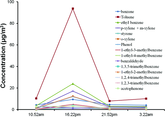Fig. 4 Concentration plotted against the starting time of sampling for various aromatic target analytes, for samples collected on 23 February 2012.

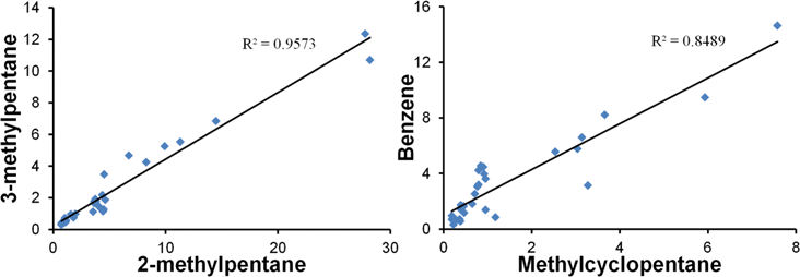Fig. 5 Correlation graph between 2 compounds (in μg m⁻³): 3-methylpentane and 2-methylpentane (left); benzene and methylcyclopentane (right).

From the amount of data obtained in February 2012, general concentration patterns of target VOCs were established and the dominant sources of hydrocarbons and aromatic compounds were estimated. However, statistical modelling is essential for accurate identification and apportionment of sources. Long-term air monitoring studies are necessary for modelling the source contribution and to accurately determine the natural variations in concentration trends.

Conclusions

A TD-GCMS method has been developed for the simultaneous detection of 47 atmospheric VOCs commonly detected in Singapore, a country with a large industrial chemical industry. Only 1 of the 47 compounds (dichloromethane) did not meet the breakthrough criteria during air sampling. All 47 compounds meet the reproducibility criteria when air was sampled using calibrated pumps.

Pyridine was not detected in the air samples collected because it was only present when the air quality was affected by the annual transboundary haze pollution caused by Indonesian forest fires. The selection of sampling volume, breakthrough, reproducibility, MDL and MQL values for pyridine remain unknown and have to be carried out during the haze period.

Samples were collected and the general concentration trends were analysed and sources were estimated for hydrocarbons and aromatic VOCs by plotting R² correlation graphs to reference indicators exclusively present in automobile emissions. Comparisons between different nations were made for high concentration VOCs such as toluene and benzene. However, the accurate determination of source contribution and concentration variations requires statistical modeling and long-term monitoring of air samples.

With a versatile method optimized, developed and validated for detecting VOCs, further studies are in progress to understand the concentration patterns of these compounds that are present in the atmosphere at different times during the day, the month and within a year in Singapore industrial and residential areas.

Acknowledgements

This work was supported by a Singapore Ministry of Education Tier 1 research grant (RG 61/11).

Notes and references

1. J. Dewulf and H. Van Langenhove, J. Chromatogr., A, 1999, 843, 163–177.
2. A. R. MacKenzie, R. M. Harrison, I. Colbeck and C. N. Hewitt, Atmos. Environ., Part A, 1991, 25A, 351–359.
3. R. G. Derwent, M. E. Jenkin and S. M. Saunders, Atmos. Environ., 1996, 30, 181–199.
4. R. Atkinson, Atmos. Environ., 2000, 34, 2063–2101.
5. C. J. Weschler and H. C. Shields, Atmos. Environ., 1997, 31, 3487–3495.
6. Agency for Toxic Substances and Diseases Registry (ATSDR), July 2011, http://www.atsdr.cdc.gov/.
7. United States Environment Protection Agency, Integrated Risk Information System (IRIS), July 2011, http://www.epa.gov/iris/index.html.
8. O. Baroja, E. Rodríguez, Z. Gomez De Balugera, A. Goicolea, N. Unceta, C. Sampedro, A. Alonso and R. J. Barrio, J. Environ. Sci. Health, Part A: Toxic/Hazard. Subst. Environ. Eng., 2005, 40, 343–367.
9. United States Environmental Protection Agency, An introduction to Indoor Air Quality (IAQ), Volatile Organic Compounds (VOCs), October 2011, http://www.epa.gov/iaq/voc2.html.
10. European Environment Agency, Non-Methane Volatile Organic Compounds (NMVOC) Emissions (APE 004), October 2011, http://www.eea.europa.eu/data-and-maps/indicators/eea-32-non-methane-volatile-1.
11. National Environment Agency, Guidelines for Good Indoor Air Quality in Office Premises, October 2011, http://www.nea.gov.sg/cms/qed/guidelines.pdf.
12. Umwelt Bundes Amt, Health and Environmental Hygiene Indoor Air Hygiene Commission (IRK), October 2011, http://www.umweltbundesamt.de/gesundheit-e/innenraumhygiene/irk.htm.
13. United States Environmental Protection Agency, Six Common Air Pollutants, October 2011, http://www.epa.gov/airquality/urbanair/.
14. Australian Government Department of Sustainability, Environment, Water, Population and Communities, Criteria pollutants, October 2011, http://www.environment.gov.au/atmosphere/airquality/publications/airtoxics.html.
15. Umwelt Bundes Amt, Current concentrations of air pollutants in Germany, October 2011, http://www.envit.de/umweltbundesamt/luftdaten/index.html?setLanguage=en.
16. N. Ramírez, A. Cuadras, E. Rovira, F. Borrull and R. M. Marcé, Talanta, 2010, 82, 719–727.
17. NIOSH, Method 1500, Issue 3, NIOSH Manual of Analytical Methods (NMAM), 4th edn, 2003.
18. NIOSH, Method 1501, Issue 3, NIOSH Manual of Analytical Methods (NMAM), 4th edn, 2003.
19. A. Rosell, J. I. Gomez-Belinchon and J. O. Grimalt, J. Chromatogr. B, 1991, 562, 493–506.
20. P. Bruno, M. Caputi, M. Caselli, G. De Gennaro and M. De Rienzo, Atmos. Environ., 2005, 39, 1347–1355.
21. S. Król, B. Zabiegała and J. Namieśnik, TrAC, Trends Anal. Chem., 2010, 29, 1101–1112.
22. E. Matisová and S. Škrabáková, J. Chromatogr., A, 1995, 707, 145–179.
23. C.-W. Chung, M. T. Morandi, T. H. Stock and M. Afshar, Environ. Sci. Technol., 1999, 33, 3661–3665.
24. C.-W. Chung, M. T. Morandi, T. H. Stock and M. Afshar, Environ. Sci. Technol., 1999, 33, 3666–3671.
25. M. R. Ras, F. Borrull and R. M. Marcé, TrAC, Trends Anal. Chem., 2009, 28, 347–361.
26. H. Skov, A. Lindskog, F. Palmgren and C. S. Christensen, Atmos. Environ., 2001, 35, S141–S148.
27. C. Y. Chan, L. Y. Chan, X. M. Wang, Y. M. Liu, S. C. Lee, S. C. Zou, G. Y. Sheng and J. M. Fu, Atmos. Environ., 2002, 36, 2039–2047.
28. A. Muezzinoglu, M. Odabasi and L. Onat, Atmos. Environ., 2001, 35, 753–760.
29. I. L. Gee and C. J. Sollars, Chemosphere, 1998, 36, 2497–2506.
30. A. Kumar and I. Víden, Environ. Monit. Assess., 2007, 131, 301–321.
31. D. K. W. Wang and C. C. Austin, Anal. Bioanal. Chem., 2006, 386, 1099–1120.
32. E. Woolfenden, J. Chromatogr., A, 2010, 1217, 2674–2684.
33. E. Woolfenden, J. Chromatogr., A, 2010, 1217, 2685–2694.
34. A. Ribes, G. Carrera, E. Gallego, X. Roca, M. J. Berenguer and X. Guardino, J. Chromatogr., A, 2007, 1140, 44–55.
35. Ö. O. Kuntasal, D. Karman, D. Wang, S. G. Tuncel and G. Tuncel, J. Chromatogr., A, 2005, 1099, 43–54.
36. U.S. EPA, Compendium of Methods for the Determination of Toxic Organic Compounds in Ambient Air, Method TO-17, Center for Environmental Research Information, Office of Research and Development, U.S. EPA, 1999.
37. Singapore Accreditation Council, Accreditation Scheme for Laboratories, Guidance Notes C & B and ENV001 Method Validation for Chemical Testing, April 2002, http://www.sac-accreditation.gov.sg/documents.asp, accessed 03 February 2010.
38. M. R. Ras-Mallorquí, R. M. Marcé -Recasens and F. Borrull-Ballarín, Talanta, 2007, 72, 941–950.
39. National Environment Agency, Singapore, September 2012, http://app2.nea.gov.sg/weather_statistics.aspx.
40. M. Harper, Ann. Occup. Hyg., 1993, 37, 65–88.
41. E. Gallego, F. J. Roca, J. F. Perales and X. Guardino, Talanta, 2011, 81, 916–924.
42. W. A. McClenny and M. Colón, J. Chromatogr., A, 1998, 813, 101–111.
43. Markes International Ltd., Confirming Sorbent Tube Retention Volumes and Checking for Analyte Breakthrough, In-house Publication, UK, 2012.
44. J. F. Pankow, W. Luo, L. M. Isabelle, D. A. Bender and R. J. Baker, Anal. Chem., 1998, 70, 5213–5221.
45. X.-L. Cao and C. N. Hewitt, J. Chromatogr., A, 1994, 688, 368–374.
46. P. Ciccioli, E. Brancaleoni, A. Cecinato, C. di Palo, A. Brachetti and A. Liberti, J. Chromatogr. A, 1986, 351, 433–449.
47. J. H. Lee, S. A. Batterman, C. Jia and S. Chernyak, J. Air Waste Manage. Assoc., 2006, 56, 1503–1517.
48. Economic Development Board, Singapore, Facts and Figures, http://www.edb.gov.sg/edb/sg/en_uk/index/industry_sectors/Chemicals/facts_and_figures.html.
49. H. Guo, T. Wang, I. J. Simpson, D. R. Blake, X. M. Yu, Y. H. Kwok and Y. S. Li, Atmos. Environ., 2004, 38, 4551–4560.
50. N. Yamamoto, H. Okayasu, S. Murayama, S. Mori, K. Hunahashi and K. Suzuki, Atmos. Environ., 2000, 34, 4441–4446.
51. K. Na, Y. P. Kim and K. C. Moon, Atmos. Environ., 2003, 37, 733–742.
52. N. Moschonas and S. Glavas, Atmos. Environ., 1996, 30, 2769–2772.
53. D. Brocco, R. Fratarcangeli, L. Lepore, M. Petricca and I. Ventrone, Atmos. Environ., 1997, 31, 557–566.
54. R. D. Edwards, J. Jurvelin, K. Saarela and M. Jantunen, Atmos. Environ., 2001, 35, 4531–4543.
55. T. Ohura, T. Amagai and M. Fusaya, Atmos. Environ., 2006, 40, 238–248.
56. P. L. Kinney, S. N. Chillrud, S. Ramstrom, J. Ross and J. D. Spengler, Environ. Health Perspect., 2002, 110, 539–546.
57. Baseline Air Toxics Project (2000), Volatile Organic Compounds Monitoring in Perth, Department of Environmental Protection, Perth, Western Australia, January 2000, http://portal.environment.wa.gov.au/pls/portal/docs/PAGE/DOE_AD-MIN/TECH_REPORTS_ROSITORY/TAB1019688/VOC_REPORT.PDF.
58. A. Srivastava, A. E. Joseph, S. Patil, A. More, R. C. Dixit and M. Prakash, Atmos. Environ., 2005, 39, 59–71.
59. L. Zhao, X. Wang, Q. He, H. Wang, G. Sheng, L. Y. Chan, J. Fu and D. R. Blake, Atmos. Environ., 2004, 38, 6177–6184.
60. J. Zhu, R. Newhook, L. Marro and C. C. Chan, Environ. Sci. Technol., 2005, 39, 3964–3971.
61. C. C. Chang, J.-L. Wang, S. C. Liu and S.-C. C. Lung, Atmos. Environ., 2006, 40, 6349–6361.
62. C. C. Chang, J.-L. Wang, S.-C. C. Lung, S.-C. Liu and C.-J. Shiu, Atmos. Environ., 2009, 43, 1771–1778.

---