DOI:
10.1039/C1SM06662E
(Paper)
Soft Matter, 2012,
8, 227-234
Received
1st September 2011
, Accepted 28th October 2011
First published on 14th November 2011
Abstract
Nanoparticles functionalized with photo-switchable ligands can be assembled into a broad range of structures by controlled light exposure. In particular, alternating light exposures provide the means to control formation of assemblies of various sizes and symmetries. Here, we use scaling arguments and Kinetic Monte Carlo simulations to study the evolution of reversible aggregates in a solution of periodically irradiated photo-switchable nanoparticles. Scaling estimates of the characteristic size and the mean separation of aggregates agree with the simulations. The transition probabilities in the Kinetic Monte Carlo scheme are derived from a renormalized master equation of the diffusion process. Simulations on a system of nanoparticles, interacting through Lennard-Jones pair potentials that change their character from repulsive to attractive depending on the light exposure, show that the slow diffusion of particles at low effective temperatures (where the attractions are much higher than the thermal energy) results in the formation of small, “kinetically frozen” aggregates. On the other hand, aggregation does not occur at high effective temperatures, where the attractions are comparable to the thermal energy. In the intermediate range of effective temperatures, “fluctuating” aggregates form that can be stabilized by applying light pulses of specific lengths and frequencies. The aggregate sizes increase by increasing the packing fraction and the aggregates undergo transition to a percolated “network” at high packing fractions. Light-control of inter-particle interactions can either inhibit or promote nucleation and growth, and can reduce gel and glass formation.
1 Introduction
Self-assembly of colloids and nanoparticles can generate a multitude of structures and patterns for a range of applications, including catalytic systems,1,2 electronic devices3,4 and colloidal inks.5,6 One of the major complications in the field is the control of the assembly process such as to avoid kinetic trapping and defect formation.7–9 Dynamic self-assembly10–13 aims at producing ordered structures “on demand” by controlled energy influx into the system. Systems are driven out of their natural (equilibrium) states and forced to adapt ordered architectures, by changes in the chemical or field-based stimuli. This strategy, developed by Whitesides and Grzybowski14,15 has been widely successful in the design of nanoscale components and systems, in cases where the conventional equilibrium design methods do not offer adequate and dynamic control over the formation of assemblies. Of the many possible candidates of the control variables, light stands out unique, as it is non-evasive and capable of instantaneous delivery at precise locations;16,17 as opposed to the relatively slow chemical delivery methods for which diffusive limitations are often present. Recent experimental efforts on the light induced self-assembly (LISA) of photo-switchable materials18 have met with considerable success, and many applications such as in self-erasable papers,6catalytic switches,1 and nanoscale temperature sensors19 are being considered.
One barrier to future developments in dynamic self-assembly is the lack of guiding general principles that would describe the behavior of systems at miniature length-scales and far-from-equilibrium. Despite long history of research—dating back to Onsager and Prigogine—non-equilibrium thermodynamics is a field still in its infancy.20 In the absence of general description of far-from-equilibrium systems, one has to resort to computational approaches which, however, are system-specific and present a multitude of technical challenges associated with tracking the dynamics of infinitely many particles that are needed to explain the mesoscale behavior of the systems under study. A useful compromise is achieved by numerical schemes based on continuum models, coarse-grained particle models, and implicit solvent models. These methods enable the possibility of simulating larger systems for longer times, at the expense of some arbitrariness in the definition of time. Phase-field approaches,21 Coarse-grained Molecular Dynamics (MD),22 and Brownian dynamics methods23 are examples of such schemes.
We propose here a scaling theory and a kinetic Monte Carlo (kMC) simulation scheme to study aggregation kinetics in a model non-equilibrium nanosystem of light-switchable nanoparticles (NPs) under periodic light forcing. As a case in point, we consider a variation of an experimental LISA process,16 where a solution of NPs functionalized with photo-switchable ligands is subjected to alternating exposures to UV and visible light (henceforth referred as “ON” and “OFF” states of light, respectively), leading to the conversion of associative NPs to non-associative NPs, and vice versa. Controlling the time duration of light exposure allows for a control of the sizes and the polydispersities of NP aggregates.6 At the same time, the periodic exposure is a test of the structural reversibility of these aggregates. This study of the phase behavior of “switchable” nanocolloids can thus provide a theoretical framework for studying “dynamic” materials whose properties derive from the ability of the components to change their interaction potentials in response to specific environmental stimuli. Also, the idea of periodic forcing of switchable NPs is motivated by the issues of energy efficiency in dynamic self-assembly where, as we show, achieving an ordered state does not necessarily require a constant flux of energy but only a properly timed sequences of “pulses” sufficient to maintain the ordered states.
2 Methodology
Fig. 1A illustrates a schematic of our model system, whereby we describe all relevant parameters of the model. The magnitude and the time span of light exposure are crucial in determining the resulting size and structure of the NP aggregates. In particular, in the case of no light exposure, all NPs are non-associative and the solution is akin to an ideal gas of particles. Under light irradiation and in the limit of very long aggregation times, all NPs are associative and one large aggregate is expected due to the Ostwald ripening effect. For intermediate values of the aggregation time, the system remains macroscopically homogeneous with local heterogeneities characterized by the separation between microscopic aggregates. Thus, it is reasonable to expect that the sizes of the NP aggregates and the separations between them can be controlled by varying the aggregation time τa and the disassembly time τd. In this spirit, the mean separation λ between the aggregates at the end of the aggregation phase, the mean free path of free NPs in the original solution λ0, and the diameter of the NPs r0, provide the relevant length scales for the problem (Fig. 1B). The packing fraction of NPs in the original solution η0 is related to λ0 by η0 = (λ0/r0)−3. The choice of τa and τd must take into account the characteristic times for the non-associative (A) ⇔ associative (B) switching of individual NPs – these times are defined as τon and τoff for the forward and backward transitions, respectively. In the scaling arguments that follow, we consider a scenario where the A ⇔ B transition is infinitely fast compared to assembly and disassembly times under different light exposures (i.e. τon ≪ τa and τoff ≪ τd). We note that this assumption is realistic for the experimental LISA systems where the isomerization of the nanoparticles (e.g., ones covered with azobenzene-dithiol ligands16) under UV light is usually much faster than the assembly or disassembly of any sizable NP aggregate. Furthermore, τd is chosen such that the system is devoid of all heterogeneities and returns to a random distribution at the end of the disassembly phase. The latter criterion draws inspiration from the recent experiments on self-erasing materials,6 where complete structural reversibility was desired. As discussed later, we use the scaling estimates to guide the kMC simulations, where these simplifying assumptions are relaxed. In order to distinguish the scaling estimates from those used in simulations, we represent the scaling estimates of τd and τa by τ and τ′, respectively.
 |
| | Fig. 1 Schematic of the LISA process with periodic light forcing. (A) Fraction of associative particles (green bold line) and light intensity (black dashed line) as a function of time. and τa are the time spent in the “disassembly” and the “aggregation” phase, where the light is turned “OFF” and “ON”, respectively. The associative ⇔ non-associative transition follows a first order kinetics, with the fraction of sticky particles given by the first order kinetics, fB = 1 − e−δt/τon (switch-on) and fB = e−δt/τoff (switch-off), δt being the time spent since the last switch-on(off) event. (B) Characteristic length scales in the disassembly and the aggregation phase. In the disassembly phase, the length scale is given by the mean free path λ0 = η−1/30r0 where η0 is the packing fraction of particles in the original solution, and r0 is the diameter of the particles. The aggregation phase has a characteristic length scale λ, which corresponds to the lattice parameter for ordered crystalline structures, and the mean distance between oscillating units for disordered fluctuating structures. | |
2.1 Scaling analysis
The characteristic time needed to completely destroy an NP aggregate is given by the familiar diffusion relation, τ = λ2/D, where D is the diffusion coefficient of the free NPs in solution. On the other hand, NP aggregation can be represented as a homogeneous nucleation process of the type B + BN = BN+1, where N(t) is the number of NPs in the aggregate at time t measured since the beginning of the aggregation phase. This description assumes active nucleation centers of number density nc = 1/λ3. The number density of free NPs (B) can be given by the first order kinetics, with the rate constant given by the Smoluchowski relation, K(t) = 4πRD, where R ∼ r0N1/3 is the radius of the aggregate. The aggregation time can be estimated by using the life time of free particles obtained from the numerical solution of the kinetic equation dn(t)/dt = −K(t)ncn(t) for the number density of free particles n(t) = n0 − nc, where n0 = 1/λ30 is the number density of the particles in the original solution. The aggregation time thus obtained is given by†| |  | (1) |
Note that τ and τ′ are not independent of each other. For a given system, an increase in τ′ must be accompanied by an increase in τ by the same factor. Finally, the maximum number of particles in an aggregate, or “aggregation number”, can be estimated by the relation, N0 = (λ/λ0)3. As an illustration, we consider the typical range of experimental parameters:1,16r0 = 5–10 nm, D = 4 × 10⁻⁷ cm2 s−1, and n0 = 1013–1014 cm−3. Then, one can estimate that the assembly and disassembly of aggregates comprising N0 = 1![[thin space (1/6-em)]](https://www.rsc.org/images/entities/char_2009.gif) 000000 particles requires exposure times of τ′ = 250–5000 s and τ = 12–54 s, which is similar in magnitude to the experimentally determined values. Moreover, τ and τ′ scales as N2/30 assuming that other system parameters are held fixed.
000000 particles requires exposure times of τ′ = 250–5000 s and τ = 12–54 s, which is similar in magnitude to the experimentally determined values. Moreover, τ and τ′ scales as N2/30 assuming that other system parameters are held fixed.
Naturally, the scaling estimates give only a rough approximation of the assembly/disassembly process and lack any information on the packing fraction and the structure of the aggregates, and the effects of the degree of particles' association and the diffusion rates. However, scaling estimates significantly reduce the microscopic parameter regime of a large number of model parameters, which needs to be explored to gain physical insights into the underlying process. Therefore, we use the scaling analysis to guide the kMC simulations, and to gain a detailed understanding of the assembly/disassembly process. Note that our current study is for a “forced dynamic self-assembly” process which does not possess a natural frequency and characteristic length scales of oscillations in the absence of periodic light switching, thus enabling us to develop analytical scaling estimates. In the more general case of “self-oscillating” systems with natural frequencies and characteristic length scales, preliminary simulations are required to establish the scaling laws.24,25
2.2 Renormalization of diffusion equations
The traditional approach of solving diffusion problems uses either the numerical solution of the deterministic Smoluchowski diffusion equation or that of a related stochastic diffusion equation using Brownian dynamics. A common problem in both methods is that the choice of time-step is limited by the values of the interaction potential and temperature. This requirement is associated with the numerical stability of these methods, and if a proper timestep is not employed, one is often faced with the challenge of error propagation with simulation time. This problem is even more exacerbated if the interaction potentials are unbounded at a certain point in space due to some constraints (e.g., in the case of hard-core potentials), where the magnitude of time step must be small enough. Moreover, in a Brownian dynamics simulation, it is practically impossible to distinguish between the stochastic terms in the equations and those that appear due to numerical error. This accumulation of numerical error manifests in uncontrolled changes in the effective diffusion constant or the type of diffusion (normal to anomalous). Further, one particular realization of the stochastic “noise” term is often not relevant (and is physically unrealistic) and we are interested in the average quantities which are obtained by averaging over many trajectories. In the following, we discuss a renormalization approach that addresses all these problems. The key ingredient in this approach is that the equations of diffusion dynamics are renormalized to a master equation with transition rates identical to the Glauber definition of transition probabilities,26 which can be efficiently solved by Monte Carlo simulations.
Let us consider the diffusion kinetics of a particle in one-dimension under the influence of an external force F(r). The probability density to find the particle at location r at time t, c(r,t), is given by the Smoluchowski equation,
where the flux
j(
r,
t) is given as,
| | | j(r,t) = D[∂rc(r,t) − βF(r)c(r,t)], | (3) |
with
β = 1/
kBT, where
kB and
T are the Boltzmann constant and temperature, respectively. For numerical convenience,
eqn (2) can be written as a difference equation of the form:
| |  | (4) |
where we assume space and time discretizations,
rm =
am and
tn =
nΔ
t. A central difference approximation is used for the space derivative of the flux and
Lm is the linear operator for the time difference. In the Forward Euler scheme,
Lmc=(
cn+1m −
cnm)/Δ
t, where
cnm indicate the probability density of the particle to be at location
rm at time
tn. Note that the simultaneous integral transformation and discretization as applied in
eqn (4) ensures that the difference scheme is conservative meaning that the total probability stays constant.
Next, we introduce an auxiliary field,
where
U(
r) is the potential energy of particle at location
r. Using
F(
r) = −
dU(
r)/
dr in
eqn (5),
eqn (3) for the flux reduces to,
| |  | (6) |
Integrating dw(r)/dr in the interval r ∈ [rm,rm+1], we get,
| |  | (7) |
where we have used the fact that
eβU(r) in the above integrand changes much rapidly than the flux
j(
r) on the scale Δ
r =
a. Using
eqn (5) and
eqn (7), we obtain the master equation,
| |  | (8) |
Here, K(m + 1 → m) and K(m → m + 1) are the dimensionless transition rates defined as,
| |  | (9) |
| |  | (10) |
The resulting form of the flux term jm+1/2 is a renormalized one, since the potential and temperature appear only inside the definition of coefficients, which are bounded. Thus, it is always possible to find a constant time step which is not a function of temperature or potential for which the numerical scheme will be stable (errors will not propagate in time). Further, it is obvious from eqn (12) and eqn (13) that the probability of transition into a non-physical zone, where Um+1 → ∞, equals zero. Eqn (9) and eqn (10) for the dimensionless transition rates are identical with the definition of transition probability in Glauber dynamics.26 Namely, for a change in state si → sj with energies Ei and Ej, the transition probability is defined as,
| |  | (11) |
Note that the transition rate defined in eqn (11) is symmetric and constrained in the interval [0,1]. At equilibrium (jm+1/2 = 0) the flux equation (eqn (8)) reduces to the Boltzmann distribution, cm+1 = cmexp[-β(Um+1 − Um)].
2.3 Kinetic monte carlo (kMC) scheme
As derived above, the numerical solution of the diffusion equation through a difference scheme can be mapped to a finite step Monte Carlo scheme with step size equal to the spatial discretization of the difference scheme. However, to complete the transformation, we need a relation for the time step in terms of the number of Monte Carlo steps and the step size in space. As an example, we consider a one-dimensional diffusion problem with a constant drift force F, such that U(r) = −Fr. In a given Monte Carlo step, a particle may move from a position rn to rn+1 ∈ {rn,rn ± a} in a time duration [tn,tn+1 = tn + Δt]. The transition probability for the movement is given according to eqn (11) as,| |  | (12) |
where the last expression is valid for small F. Note that the probabilities defined above are for the cases when the direction of movement is first picked at random (with a probability 1/2 for both + and − directions), and the particle can stay at its original position with a probability 1/2. Thus, the mean drift is given by the relation:| |  | (13) |
Now, the mobility can be defined as,
| |  | (14) |
Finally, using the Einstein's relation, D = μ/β, we can find the definition of timestep as, Δt = a2/4D. This result can be easily generalized to an arbitrary dimension d as,
| |  | (15) |
The recipe of a kMC simulation using Glauber dynamics is similar to the conventional Metropolis scheme,27 but with transition probabilities defined as
| |  | (16) |
for a transition with the energy change Δ
E. Further, the choice of particle displacements is limited to the continuum version of flip movements of lattice simulations. In other words, the attempted moves of particles are constrained to lie on a surface of a sphere of radius
a centered at the “old” position, where
a is the step size. We perform three-dimensional kMC simulations of a system of NPs, placed in a large cubic box with periodic boundary conditions. The simulation box is composed of cubic cells of size
λ (
Fig. 1B). The number of such cubic cells provides a rough measure of the number of aggregates expected in a simulation, as estimated by the scaling arguments. Note that the cubic grid is employed only to obtain better statistical measures and to minimize periodicity artifacts; it does not play any role in the evaluation of energetic interactions. We use a simulation box with 5
3 = 125 cubic cells in all simulations. A kMC step consists of attempted moves of all particles, decided by the choice of the azimuthal angle
ϑ = 2π
u and the polar angle
ϕ =
acos(2
v − 1),
28 where
u and
v are random variables in (1,3). The attempted moves are accepted with the transition probability given by
eqn (16). The “new” positions of particles, if a move is accepted, is stored in a coordinate array, and is copied into the particle coordinates once all particles have moved. Each kMC step corresponds to a step in time given by
eqn (15), that is, for
d = 3,
| |  | (17) |
where
τ0 =
r20/
D is a convenient unit of time. We use
a = 0.1
r0 in our simulations. This choice gives reasonable acceptance rates of particle movements. The degree of association is characterized by a dimensionless temperature
θ ≡
T/
T0, where
T and
kBT0 are the temperature and the depth of the LJ potential, respectively. The interactions between particles at distance
r are modeled using a shifted LJ potential of the form:
| |  | (18) |
The tail-correction ε is chosen such that U(rcut) = 0 for a cutoff distance rcut. We choose rcut = 21/6r0 for interactions involving non-associative particles, to mimic purely repulsive hard cores of particles. A higher cutoff value of rcut = 2.5r0 is used for short-range attraction between associative particles, with the cutoff chosen for efficiency in the implementation.
The effective diffusion rates of NPs inside the aggregates are different from those of free NPs in dilute solution – characterized by the diffusion constant D. Indeed, the effective diffusion of NPs depends also on the local concentration, which is often described in a phenomenological manner by including arbitrary concentration dependence in D. Such ad hoc modification is not required in the current model, because the diffusion of NPs inside the aggregates is naturally reduced by the presence of nearby particles, as reflected in the acceptance rates of kMC moves. For example, at low temperatures, NPs diffuse slower inside the aggregates (low acceptance rates) than compared to the high temperature case or the free NPs in solution (high acceptance rates). Further, since our objective is to capture the true dynamics at short time-scales and not the equilibrium phase behavior at long time scales, we refrain from the use of collective moves that would necessitate the definition of multiple time scales.
2.4 Characterization of aggregates
The aggregate size distribution is sampled by counting the number of aggregates ni, with an aggregation number i, which is defined as the number of particles in the aggregate (i = 1,2…). Two particles are considered to be the part of an aggregate if the distance between them is less than 1.5r0.‡ Aggregate size distributions are used to compute the number average aggregate size  and the weight average aggregate size
  . The polydispersity of the aggregates is defined as the ratio Mw/Mn and is equal to 1 for mono-dispersed aggregates. The radial distribution function is averaged over all particles in the simulation box at a given instant of time (not time-averaged) and obtained by the standard binning procedure.29 Local bond order parameter q6 for particle i is defined as,30
| |  | (19) |
where the local bond orientational order parameter ![[q with combining macron]](https://www.rsc.org/images/entities/i_char_0071_0304.gif) 6m(i) is given by,
6m(i) is given by,| |  | (20) |
Here, Y6m(![[r with combining circumflex]](https://www.rsc.org/images/entities/b_i_char_0072_0302.gif) ij) are the spherical harmonics of order six, ij are the unit vectors connecting the particle i with its nearest neighbors and Nb(i) is the total number of nearest neighbors of particle i. The nearest neighbors are found using a parameter-free neighbor search algorithm.31
ij) are the spherical harmonics of order six, ij are the unit vectors connecting the particle i with its nearest neighbors and Nb(i) is the total number of nearest neighbors of particle i. The nearest neighbors are found using a parameter-free neighbor search algorithm.31
3 Results and discussion
3.1 Aggregate size
To quantify the effects of the degree of association and nanoparticle concentration, we analyze the system behavior for a range of dimensionless temperatures, θ, and packing fractions of particles in the original solution, η0 after one cycle of light exposure (Fig. 2 and Fig. 3). At low temperatures (θ = 0.05 in Fig. 2A), the system favors small, “kinetically frozen” aggregates with high degrees of symmetry. An increase in θ beyond this limit leads to an increase in size of the aggregates (θ = 0.2 in Fig. 2A) and the system favors “flexible” structures with fluctuating particles that remain in the aggregate. Increasing θ further results in “highly fluctuating” aggregates, which often dissociate and re-combine with the constituent NPs (θ = 0.6 in Fig. 2A). At even higher values of θ (θ = 1.0 in Fig. 2A), aggregation does not occur. This non-monotonic dependence on θ arises from the competition of energetic and kinetic effects. While the energetic interactions due to the association of particles decrease with an increase in θ, the effective diffusion rates increase with increasing θ. Therefore, the system tends to favor small, relatively mono-dispersed aggregates at low θ, which increase in size until θ reaches a threshold temperature, where the kinetic effects become dominant (between θ = 0.3 and θ = 0.4 in Fig. 3A). Beyond this threshold temperature, the aggregates begin to dissociate and re-combine and form highly fluctuating poly-dispersed structures, and no aggregation occurs at very high θ (θ > 0.7 in Fig. 3A). An increase in η0 leads to an increase in the size of aggregates (Fig. 2B and Fig. 3B) eventually leading to the formation of percolated “network” structures (η0 = 0.2963 in Fig. 2B).
 |
| | Fig. 2 Typical simulation snapshots at the end of aggregation phase after one cycle of light exposure. Snapshots are zoomed in to show individual aggregates in detail and do not show the entire simulation box. The contrast (bold or faded) of particles is used to indicate the depth of particles from the top plane (close or farther). (A) For a range of θ with η0 = 0.037. (B) For a range of η0 with θ = 0.2. τd = τ, τa = τη−1/30 and λ/λ0 = 4 for all snapshots. The relaxation process is assumed to be infinitely fast. | |
 |
| | Fig. 3 Number average aggregate size (Mn) and polydispersity (PD) of the aggregates at the end of aggregation phase after one cycle of light exposure. Variation of Mn and PD with (A) temperature θ ≡ T/T0 for η0 = 0.037, (B) with η0 for θ = 0.2. The model parameters are τa = τη−1/30, τd = τ, and λ/λ0 = 4. The relaxation process is assumed to be infinitely fast. Error bars have roughly the size of the symbol and represent the numerical error as opposed to the error resulting from the presence of stochastic term in Brownian dynamics. | |
It is useful to note here that the effective temperature θ in this study is introduced as a measure of the degree of association and should not be interpreted as the actual temperature of the system at thermodynamic equilibrium. Indeed, the non-monotonic dependence of the aggregate size on θ is a consequence of the fact that the systems at different values of θ are subjected to equal exposure times, which are estimated by scaling arguments. We believe that the systems at low temperatures would tend to form much larger aggregates, if they are allowed sufficiently long time in the aggregation phase. However, the dissociation and re-combination of aggregates at high θ is expected to be present even at high temperatures in thermodynamic equilibrium, where the magnitude of inter-particle attractions is comparable to that of thermal fluctuations.
3.2 Aggregate structure
In Fig. 4A and Fig. 4B, we show the radial distribution function g(r/r0) at the end of one cycle of light exposure. The sharp peaks in g(r/r0) are indicative of the development of a local order inside the aggregates. The features in g(r/r0) are enhanced with a moderate increase in θ (θ = 0.05–0.2 in Fig. 4A) and as η0 increases (Fig. 4B) due to the increase in the number of layers of particles in the aggregates. However, the features disappear with a further increase in θ (θ = 0.4–0.8 in Fig. 4A) after the onset of dissociation and recombination of aggregates. It is difficult to quantify the crystallinity of aggregates of fewer than hundred particles observed in this study. The conventional procedure of crystal structure determination in simulations defines a particle to be “crystalline” or “solid-like” if the local neighborhood of the particle is identical (or strongly correlated) with its neighbors,30,32 as determined by the correlations of the Steinhardt order arameters33 or its modifications.34 Such criterion is indeed not met in small nano-clusters, with few layers of particles and large surface to volume ratios. We use the distribution of local bond order parameter q6 (Fig. 4C and Fig. 4D) as a probe to the development of crystalline order on an individual particle level.30,32,33 We find that the distributions at low θ (Fig. 4C) and low η0 (Fig. 4D) are shifted towards high q6, indicating that the particles inside the aggregates are more crystalline in these cases. At low θ, particles pack tightly because of high inter-particle attractions, giving rise to a crystal-like ordering (or, for few particles, symmetric structures). On the other hand, at low η0, the aggregates are less fluctuating as opposed to the high η0 case where the crowding of particles leads to competing attractions from all the neighbors leading to higher flexibility. However, we did not observe a narrowing of q6 distribution, as one would expect for perfect crystalline structures.32 With regards to the actual LISA experiments, we observe that a covalent cross-linking (of thiol groups) in addition to the short-range dipole–dipole attractions was necessary to induce perfect crystalline order,16 and high quality crystals were not formed in the absence of this crosslinking.6 However, the existence of such crosslinking renders the structures irreversible, as it is difficult to break the covalent bonds after it is formed.
 |
| | Fig. 4 Radial Distribution function and local bond order parameter (q6) distributions. Radial distribution function: (A) for a range of θ with η0 = 0.037, (B) for a range of η0 with θ = 0.2. Probability density distribution of q6: (C) for a range of θ with η0 = 0.037, (D) for a range of η0 with θ = 0.2. The model parameters are τd = τ, τa = τη−1/30 and λ/λ0 = 4. The relaxation process is assumed to be infinitely fast. | |
3.3 Reversibility and relaxation
We have so far considered the final state of the system at the end of the first cycle of light exposure and assuming that the relaxation process is infinitely fast. Fig. 5 shows the system behavior after five cycles for different disassembly times, wherein the associative → non-associative transition occurs with a finite relaxation time such that the aggregates do not dissolve completely in the disassembly phase. The non-associative → associative transition is assumed to be infinitely fast, as in the previous discussion. This particular choice is guided by the experimental observation that the associative NPs in the aggregates take longer to switch to non-associative when the light is turned OFF, as opposed to the relatively fast switching of particles when the light is turned ON.6,16 Aggregates evolve in a nonlinear way with larger rates of evolution at the beginning of the aggregation phase, and smaller rates towards the end of the aggregation phase. We observe that short disassembly times (τd = 0.05τ − 0.2τ) do not significantly affect the final aggregate size, when compared to the case where the light is kept ON for the same period (τd = 0). In fact, it may lead to an increase in the aggregate size, as observed for t > 1500τ0 in the figure. This is because short disassembly times allow the aggregates to re-organize; they evolve at a faster rate when light is turned ON again. For intermediate disassembly times (τd = 0.5τ), the system evolves into smaller aggregates when compared to the τd = 0 case. For even higher disassembly times (τd = τ), the aggregation behavior is completely reversible and the aggregates evolve to approximately the same size after every cycle of light exposure. We performed this analysis for a range of θ values (not shown) and analyzed the temperature dependence of aggregate size at various values of τd for different cycles of light exposure. Typically, the choice of τd has smaller influence on aggregate size for high values of θ where diffusion effects are dominant meaning that the aggregates evolve to similar sizes after the light is switched off for a certain period, when compared to the case when the light is ON for the entire period. However, τd has a stronger influence for low values of θ, where the attractive forces are dominant, and an increase in τd beyond a certain value (τd > 0.2τ in Fig. 5) gives rise to smaller aggregates. Thus, the frequency of light exposure in combination with the exposure times can be used as a design variable to form aggregates of a desired size and reversibility.
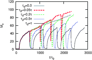 |
| | Fig. 5 Aggregate size evolution with time and the effect of relaxation. The model parameters are η0 = 0.037, τa = τη−1/30, λ/λ0 = 4, and θ = 0.2. The switch-on process is assumed to be infinitely fast but the switch-off process has a finite relaxation time τoff = τ. The results are for five ON-OFF cycles. | |
The behavior shown in Fig. 5 exhibit striking similarities with the photo-initiated free-radical polymerization process of vinyl monomers.35 The free-radical polymerization process contains an initiation step where the free radicals are formed from initiators (such as peroxides) followed by a propagation step wherein the polymer chains absorb these radicals to form longer chains. Polymerization terminates when these radicals combine leaving no free radicals. The rate of initiation and propagation steps is proportional to the intensity of light exposure and thus can be stopped by switching off light, while radicals may still combine thus reducing their concentration. The initiation/propagation and termination steps in this process are analogous to the aggregation and disassembly of NPs in the LISA process, except that in the free radical polymerization, the polymer chains once formed cannot degrade, as opposed to the forming and breaking of the assemblies in the LISA process. Therefore, the concentration of free radicals in solution shows a trend similar to that depicted in Fig. 5 for the aggregate size.
4 Conclusions
We develop here a combination of scaling theory and kinetic Monte Carlo scheme to analyze switchable self-assembly processes of nanoparticles. The model we implemented entailed simple potentials but its general features are representative of the experimental light-switchable nanosystems.1,6,16 The system density and temperature (degree of association) are found to have a profound influence on the aggregation dynamics and on the resulting aggregate size distribution of the particles. Our model predicts the formation of fluctuating (or “flexible”) and “kinetically frozen” structures with varying degrees of association and packing fractions of the original solution, in agreement with the experiments.16 We also find network structures that resemble spinodal decomposition patterns for high packing fractions.36 The competition between energetic and kinetic effects in light-controlled self-assembly affects local and global order of the forming structures. The local order of the aggregates, which is characterized here by the radial distribution function and the local bond parameter distribution, show a tendency to crystal-like ordering at low degrees of association and low packing fractions of the original solution. This provides a route to avoid frozen, disordered glass-like structures characteristic of many aggregating colloidal systems.7 Finally, we establish that the exposure times and the frequency of light exposure are important design variables to achieve structures with a desired size and reversibility.
The kinetic Monte Carlo scheme developed here provides several advantages over the conventional dynamical simulation methods (e.g., Brownian dynamics). Since particle displacements are accepted/rejected in a Monte Carlo fashion, as opposed to moving particles following a stochastic equation of motion, unphysical movements (e.g., violation of a hard core assumption) are not possible (these moves have zero acceptance). Further, the absence of a stochastic “noise” term resolves the computational difficulties associated with generating statistically independent trajectories with definitive mean properties. This advantage is particularly relevant for cases where the magnitude of the driving force is comparable to the stochastic noise in Brownian dynamics, such as in nucleation processes when Zeldovich factors are small or phase segregation process that occur close to critical points as well as the initial kinetics of phase segregation near spinodal decomposition lines. Finally, since the timestep is independent of the magnitude of the interaction forces, much longer time-steps can be employed than the conventional Brownian dynamics technique. It would be interesting to compare the accuracy and performance of this scheme for model systems to gain a detailed understanding of these differences.
The theoretical methods we described can be extended to study light induced aggregation in systems with more complex interactions, such as electrostatic interactions, providing a possibility to control re-entrant transitions characteristic of colloidal assembly37,38 through the competition of short- and long- range interactions. In the future, it would be interesting to study systems of switchable colloids that can interact irreversibly (as in experiments where light-irradiation induces crosslinking of the NPs by covalent bonds). Our work shows that the kinetic Monte Carlo scheme for continuum (off-lattice) reaction-diffusion problems in soft-matter systems has great potential for large-scale simulations of non-equilibrium microstructures. The method can be extended to the design of specific morphologies and symmetries and to explore emergent phenomena by switching periodically and non-periodically the nature of the inter-particle interactions.
Acknowledgements
This work was supported by the Nonequilibrium Energy Research Center, which is an Energy Frontier Research Center funded by the U.S. Department of Energy, Office of Science, Office of Basic Energy Sciences under Award Number DE-SC0000989.
References
- Y. H. Wei, S. B. Han, J. Kim, S. L. Soh and B. A. Grzybowski, J. Am. Chem. Soc., 2010, 132, 11018–11020 CrossRef CAS.
- T. H. Galow, U. Drechsler, J. A. Hanson and V. M. Rotello, Chem. Commun., 2002, 1076–1077 RSC.
- A. J. Baca, J.-H. Ahn, Y. Sun, M. A. Meitl, E. Menard, H.-S. Kim, W. M. Choi, D.-H. Kim, Y. Huang and J. A. Rogers, Angew. Chem., Int. Ed., 2008, 47, 5524–5542 CrossRef CAS.
- D. V. Talapin, J. S. Lee, M. V. Kovalenko and E. V. Shevchenko, Chem. Rev., 2010, 110, 389–458 CrossRef CAS.
- J. C. Conrad, S. R. Ferreira, J. Yoshikawa, R. F. Shepherd, B. Y. Ahn and J. A. Lewis, Curr. Opin. Colloid Interface Sci., 2011, 16, 71–79 Search PubMed.
- R. Klajn, P. J. Wesson, K. J. M. Bishop and B. A. Grzybowski, Angew. Chem., Int. Ed., 2009, 48, 7035–7039 CrossRef CAS.
- M. E. Cates, Annales Henri Poincaré, 2003, 4, S647–S661 Search PubMed.
- K. A. Dawson, G. Foffi, F. Sciortino, P. Tartaglia and E. Zaccarelli, J. Phys.: Condens. Matter, 2001, 13, 9113–9126 Search PubMed.
- D. Chandler, Proc. Natl. Acad. Sci. U. S. A., 2009, 106, 15111–15112 Search PubMed.
- B. A. Grzybowski and C. J. Campbell, Chem. Eng. Sci., 2004, 59, 1667–1676 CrossRef CAS.
- M. Fialkowski, K. J. M. Bishop, R. Klajn, S. K. Smoukov, C. J. Campbell and B. A. Grzybowski, J. Phys. Chem. B, 2006, 110, 2482–2496 CrossRef CAS.
- B. A. Grzybowski, C. E. Wilmer, J. Kim, K. P. Browne and K. J. M. Bishop, Soft Matter, 2009, 5, 1110–1128 RSC.
- S. Mann, Nat. Mater., 2009, 8, 781–792 CrossRef CAS.
- G. M. Whitesides and B. Grzybowski, Science, 2002, 295, 2418–2421 CrossRef CAS.
- B. A. Grzybowski, H. A. Stone and G. M. Whitesides, Nature, 2000, 405, 1033–1036 CrossRef CAS.
- R. Klajn, K. J. M. Bishop and B. A. Grzybowski, Proc. Natl. Acad. Sci. U. S. A., 2007, 104, 10305–10309 CrossRef CAS.
- Q. Tran-Cong-Miyata, S. Nishigami, T. Ito, S. Komatsu and T. Norisuye, Nat. Mater., 2004, 3, 448–451 CrossRef CAS.
- M. M. Russew and S. Hecht, Adv. Mater., 2010, 22, 3348–3360 CrossRef CAS.
- R. Klajn, K. P. Browne, S. Soh and B. A. Grzybowski, Small, 2010, 6, 1385–1387 Search PubMed.
- M. Kröger, Phys. Rep.-Rev. Sec. Phys. Lett., 2004, 390, 453–551 Search PubMed.
- K. Thornton, J. Ågren and P. W. Voorhees, Acta Mater., 2003, 51, 5675–5710 CrossRef CAS.
- C. Reichhardt and C. J. O. Reichhardt, Phys. Rev. Lett., 2011, 106 Search PubMed.
- S. H. Northrup, S. A. Allison and J. A. Mccammon, J. Chem. Phys., 1984, 80, 1517–1526 CrossRef CAS.
- O. Kortlüke, V. N. Kuzovkov and W. von Niessen, Phys. Rev. Lett., 1999, 83, 3089–3092 CrossRef CAS.
- O. Kortlüke, V. N. Kuzovkov and W. von Niessen, Phys. Rev. E, 2002, 66 Search PubMed.
- R. J. Glauber, J. Math. Phys., 1963, 4, 294–307 CrossRef.
-
D. Frenkel and B. Smit, Understanding Molecular Simulation, Academic Press, 2001 Search PubMed.
-
E. W. Weisstein, From MathWorld–A Wolfram Web Resource.
-
M. P. Allen and D. J. Tildesley, Computer Simulation of Liquids, Oxford University Press, USA, 1989 Search PubMed.
- P. R. ten Wolde, M. J. Ruiz-Montero and D. Frenkel, J. Chem. Phys., 1999, 110, 1591–1599 CrossRef CAS.
-
J. A. van Meel, Dissertation, Van't Hoff Institute for Molecular Sciences (HIMS), 2009.
- S. Auer and D. Frenkel, Adv. Polym. Sci., 2005, 173, 149–208 CAS.
- P. J. Steinhardt, D. R. Nelson and M. Ronchetti, Phys. Rev. B, 1983, 28, 784–805 CrossRef CAS.
- W. Lechner and C. Dellago, J. Chem. Phys., 2008, 129, 114707 CrossRef.
-
P. J. Flory, Principles of polymer chemistry, Cornell University Press, Ithaca, 1953 Search PubMed.
- P. J. Lu, E. Zaccarelli, F. Ciulla, A. B. Schofield, F. Sciortino and D. A. Weitz, Nature, 2008, 453, 499–U494 CrossRef CAS.
- Y. L. Chen and K. S. Schweizer, J. Chem. Phys., 2004, 120, 7212–7222 CrossRef CAS.
- A. P. Hynninen and M. Dijkstra, Phys. Rev. Lett., 2005, 94.
Footnotes |
| † The numerical solution of the kinetic equation results in a prefactor of the order unity on the right hand side of eqn (1) that is not considered in the scaling estimates. |
| ‡ The threshold distance must be chosen to be higher than the particle diameter r0 and less than the cut-off distance of LJ interaction (rcut = 2.5r0 in our case). In general, the aggregates are loosely packed structures with mean distance between particles substantially higher than in the close packing limit (=r0). |
|
| This journal is © The Royal Society of Chemistry 2012 |
Click here to see how this site uses Cookies. View our privacy policy here.