Superconductivity in 4-Angstrom carbon nanotubes—a short review
Zhe
Wang
,
Wu
Shi
,
Rolf
Lortz
and
Ping
Sheng
*
Department of Physics and William Mong Institute of Nano Science and Technology, Hong Kong University of Science and Technology, Clear Water Bay, Kowloon, Hong Kong, China. E-mail: sheng@ust.hk
First published on 21st November 2011
Abstract
We give an up-to-date review of the superconducting phenomena in 4-Angstrom carbon nanotubes embedded in aligned linear pores of the AlPO4-5 (AFI) zeolite, first discovered in 2001 as a fluctuation Meissner effect. With the introduction of a new approach to sample synthesis around 2007, new data confirming the superconductivity have been obtained. These comprise electrical, specific heat, and magnetic measurements which together yield a consistent yet complex physical picture of the superconducting state, largely owing to the one-dimensional (1D) nature of the 4-Angstrom carbon nanotubes. For the electrical transport characteristics, two types of superconducting resistive behaviors were reproducibly observed in different samples. The first type is the quasi 1D fluctuation superconductivity that exhibits a smooth resistance drop with decreasing temperature, initiating at 15 K. At low temperatures the differential resistance also shows a smooth increase with increasing bias current (voltage). Both are unaffected by an applied magnetic field up to 11 Tesla. These manifestations are shown to be consistent with those of a quasi 1D superconductor with thermally activated phase slips as predicted by the Langer–Ambegaokar–McCumber–Halperin (LAMH) theory. The second type is the quasi 1D to 3D superconducting crossover transition, which was observed to initiate at 15 K with a slow resistance decrease switching to a sharp order of magnitude drop at ∼7.5 K. The latter exhibits anisotropic magnetic field dependence and is attributed to a Berezinskii–Kosterlitz–Thouless (BKT)-like transition that establishes quasi-long-range order in the plane transverse to the c-axis of the aligned nanotubes, thereby mediating a 1D to 3D crossover. The electrical data are complemented by magnetic and thermal specific heat bulk measurements. By using both the SQUID VSM and the magnetic torque technique, the onset of diamagnetism was observed to occur at ∼15 K, with a rapid increase of the diamagnetic moment below ∼7 K. The zero-field-cooled and field-cooled branches deviated from each other below 7 K, indicating the establishment of a 3D Meissner state with macroscopic phase coherence. The superconductivity is further supported by the specific heat measurements, which show an anomaly with onset at 15 K and a peak at 11–12 K. In the 3D superconducting state, the nanotube arrays constitute a type-II anisotropic superconductor with Hc1 ≈ 60 to 150 Oe, coherence length ξ ≈ 5 to 15 nm, London penetration length λ ≈ 1.5 µm, and Ginzburg–Landau κ ≈ 100. We give a physical interpretation to the observed phenomena and note the challenges and prospects ahead.
 Zhe Wang | Zhe Wang was born in Hunan Province, P. R. China in 1984. He obtained his BSc degree in Physics from Wuhan University in 2006 and PhD degree in Physics at the Hong Kong University of Science and Technology in 2011 under the supervision of Prof. Ping Sheng. In his PhD study, Zhe Wang mainly focused on the electrical transport measurements of carbon nanotubes at low temperatures. He also contributed to the fabrication of devices with double-wall carbon nanotubes, using focused ion beam and e-beam lithography. |
 Wu Shi | Wu Shi was born in Hubei Province, P. R. China in 1984. He obtained his bachelor's degree in Physics from Tsinghua University in 2006. Just recently he has received his PhD degree under the supervision of Prof. Ping Sheng at the Hong Kong University of Science and Technology. He is now a postdoctoral researcher in Prof. Yoshihiro Iwasa's group at the Department of Applied Physics, the University of Tokyo. His current research mainly focuses on transport properties of electric double layer transistor (EDLT) devices fabricated from light-element hosts. |
 Rolf Lortz | Rolf Lortz is an expert on calorimetric techniques in superconductors. He received his PhD in 2002 from the University of Karlsruhe in Germany, with research on high-Tc superconductors. After moving to the University of Geneva, Switzerland, in 2003, he worked on a range of exotic superconductors and discovered the first realization of a Fulde–Ferrell–Larkin–Ovchinnikov state in an organic superconductor. In 2008 he took up a position of assistant professor in the Department of Physics at the Hong Kong University of Science & Technology. Since then, he has succeeded in detecting the thermodynamic and magnetic signatures of superconductivity in carbon nanotubes. |
 Ping Sheng | Ping Sheng is the William Mong Chair Professor of Nanoscience at the Department of Physics, Hong Kong University of Science and Technology. He obtained his BSc in Physics from Caltech in 1967 and PhD in Physics from Princeton in 1971. He joined HKUST in 1994 after six years at the Sarnoff Research Lab in Princeton as a member of technical staff, and fifteen years at the Exxon Corporate Research Lab at Clinton, NJ, as a senior research associate. His current research interests include superconductivity in carbon nanotubes, acoustic metamaterials, giant electrorheological fluids, and hydrodynamic boundary condition at the fluid–solid interface. |
1. Introduction
The discovery of carbon nanotubes (CNTs)1,2 has attracted global attention mainly owing to the novel structural, mechanical and electronic properties of this unique material system.3–10 Among these properties, intrinsic superconductivity in CNTs has been a topic of the most intriguing interest. In contrast to high Tc superconductivity where the focus is on the high transition temperature, nanotube superconductivity is intriguing mainly because of the “near impossibility” of such a scenario. First, carbon is not known to be a superconducting element. Hence for CNTs to be superconducting the geometric shape of the nanotubes and their one dimensional (1D) character must play a role. That by itself would be unprecedented in the sense that one can make a material superconducting by nano-structuring. Second, even if the CNTs can have superconducting tendencies, the manifestation of superconductivity should be quenched by the long wavelength thermal fluctuations as dictated by the Hohenberg–Mermin Theorem for 1D systems,11,12 as well as by the competing mechanism of the Peierls distortion that favors a semiconducting ground state.13 Thus in spite of the theoretical prediction that small CNTs can be potential superconductors, owing to the curvature effect that opens the electron–phonon interaction channels,14 early experimental results reported for different CNT systems15–18 were greeted with skepticism. Other than the above-stated reasons, this is because only three groups have observed superconductivity in carbon nanotubes,15,17,18 and even for these three groups no consistent sets of data, which should comprise electrical, magnetic, and thermal specific heat measurements, were obtained until recently.19–21This review serves to gather all the experimental evidence for superconductivity in one type of carbon nanotube—the 4-Angstrom single-walled carbon nanotubes (SWNTs) embedded in AlPO4-5 zeolite template. The experimental data offer some answers to how the superconductivity can appear in spite of the various above-stated obstacles. The physical picture that emerges is a fairly complex one showing fluctuating quasi 1D superconducting behavior initiating at 15 K with a crossover to 3D superconductivity via coupling between the aligned nanotubes20 at around 6–7.5 K. This picture is supported by the consistency of the electrical, magnetic, and thermal data.19–21 In the 3D superconducting state, the nanotube arrays constitute a type-II, anisotropic superconductor with a Hc1 = 60–150 Oe, a coherence length ξ ≈ 5 to 15 nm, a London penetration length λ ≈ 1.5 µm, and a Ginzburg–Landau κ ≈ 100.
In what follows, Section 2 introduces the 4-Angstrom SWNTs and the early discovery of superconductivity in this system, evidenced by the fluctuation Meissner effect with a mean field critical temperature of 15 K.15 We include in Section 2 a brief review of the relevant theoretical works stimulated by this first observation. In Section 3 we summarize the experimental observations of intrinsic superconductivity in other CNT systems. Section 4 presents the new approach of sample synthesis and the related characterizations of the samples fabricated. This is followed by a description of the electrical measurements and their physical interpretation in Section 5. Sections 6 and 7 present the results of the bulk magnetic and thermal specific heat measurements, which display consistency with the electrical data. In Section 8 we conclude by addressing, in light of the results presented, some often-raised issues as well as stating the challenges and future prospects.
Three appendices follow the main text. For the purpose of easy access we summarize in Appendix A the superconducting parameter values deduced from the electrical, magnetic, and thermal specific heat measurements. Appendix B presents a heuristic description of the Hohenberg–Mermin Theorem11,12 (on the effect of thermal fluctuations) and the Peierls distortion,13 both important competing mechanisms against nanotube superconductivity. A brief account of the theory of the 1D superconductor, based on the Ginzburg–Landau equation, is given in Appendix C.
2. Basic characteristics of 4-Angstrom carbon nanotubes
2.1. Structure and geometry
Discovered in 1999, 4-Angstrom SWNTs constitute the smallest CNTs in the world.22,23 The 4-Angstrom SWNTs are embedded in the linear channels of AlPO4-5 zeolite crystal (IUPA code: AFI), which is a member of the aluminophosphate zeolite family. As illustrated in Fig. 1a, the AFI framework consists of alternating tetrahedral (AlO4)− and (PO4)+ units that form parallel, open, linear channels with a triangular lattice structure in the ab plane perpendicular to the channel axis direction, denoted the c-axis. The inner diameter of the 12-sided-ring channel is 0.73 nm after discounting the size of the oxygen atoms lining the walls, and the distance between two neighboring parallel channels is 1.37 nm. The AFI single crystals are grown by hydrothermal synthesis in Teflon-lined autoclaves,24 and Fig. 1b shows an optical image of pure AFI crystals, which are transparent with a typical size of 100 × 100 × 500 µm3. In the process of growing the AFI crystals, the TPA (tripropylamine) molecules are encapsulated in the channels of the AFI crystals as precursors. The old method of growing 4-Angstrom SWNTs was to heat the AFI crystals in vacuum at 580 °C for several hours, and some carbon atoms from the decomposition of the TPA molecules formed 4-Angstrom SWNTs, owing to the weak catalytic effect of the AFI crystals. An optical image of the AFI crystals with embedded SWNTs is shown in Fig. 1c. These crystals have been shown to exhibit strong optical anisotropy.22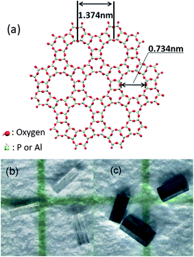 | ||
| Fig. 1 (a) The framework structure of the AFI crystal viewed along the c-axis. (b) Optical image of pure AFI crystals. (c) Optical image of AFI zeolite crystals with embedded SWNTs. | ||
The SWNTs were observed by high resolution transmission electron microscopy (HRTEM) after dissolving the AFI framework.23Fig. 2 shows a typical HRTEM image. There are two main types of morphology in the image: One type comprises the highly curved, raft-like graphite stripes indicated by “G”, and others are the paired dark narrow long fingers of ultrathin SWNTs indicated by “T”. By using the {002} spacing of the graphite (in the same image) as the internal reference, the diameter of the SWNTs was determined to be 0.42 ± 0.2 nm. Since the inner diameter of the AFI channel is 0.73 nm, and if we take the separation between the graphite sheets, 0.34 nm, as the distance between the SWNTs and the oxygen atoms lining the channel wall, then the diameter of the SWNTs should be 0.39 nm. This value is in good agreement with the HRTEM result. A value of the nanotube diameter, about 4 Angstroms, was also obtained by X-ray scattering experiments using synchrotron radiation.25
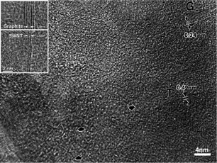 | ||
| Fig. 2 HRTEM image of 4-Angstrom SWNTs. Adapted from ref. 23. | ||
2.2. Raman characteristics
With such a small diameter, there are only three possible CNTs: (4,2), (5,0) and (3,3). It is well known that the radial breathing mode (RBM) in the Raman spectra is often useful for identifying the existence of the CNTs as well as their diameters.26 As shown in Fig. 3, Raman spectrum of the 4-Angstrom carbon nanotubes is characterized by three significant peaks at 510 cm−1, 550 cm−1, 580 cm−1 in the RBM region, attributable to the (4,2), (5,0) and (3,3) nanotubes, respectively.27 It is noted that the D band splits into three major peaks, a phenomenon which still remains unexplained. It should be noted that the large curvature of the ultra-small SWNTs introduces a re-hybridization of the σ* and π* bands, thereby leading to a softening of the RBM mode.28 This hybridization of the σ* and π* bands also greatly affects the electronic band structure of the nanotubes. To get an accurate band structure of the three types of 4-Angstrom carbon nanotubes, ab initio calculations have been performed by using a plane wave pseudopotential formulation within the framework of local density approximation (LDA).29 The (5,0) nanotube is found to be metallic, and the density of state (DOS) at the Fermi level is fairly large (0.35 states/eV per atom), making it a potential 1D superconductor. The (3,3) tube is metallic as required by symmetry considerations, and the (4,2) tube is semiconducting with a small indirect band gap of 0.2 eV. The superconducting behavior is attributed to the (5,0) carbon nanotubes.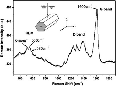 | ||
| Fig. 3 The Raman spectrum of 4-Angstrom SWNTs for ZZ polarization configuration. | ||
The imaginary part of the dielectric function for the SWNTs was calculated by the same ab initio calculations, as optical dipole transitions can occur between the van Hove singularities with specific selection rules. The resulting predictions agreed well with the polarized absorption results.22
2.3. First observation of superconductivity
The fluctuation Meissner effect was observed15 in the 4-Angstrom SWNTs in 2001, shown in Fig. 4. In that experiment, two samples were prepared: sample A consisted of pure AFI crystals (with empty pores) while sample B consisted of similar crystallites with embedded SWNTs. The crystallites in both samples were aligned to form a parallel array. Sample A showed a small, temperature independent diamagnetic signal together with a paramagnetic component. Both were isotropic with respect to the applied magnetic field. In contrast, sample B's magnetization exhibited anisotropy. Fig. 4 shows the anisotropic component of the magnetic susceptibility after subtracting the pure AFI crystals' contribution. A temperature dependent (anisotropic) diamagnetism can be clearly seen below 10 K, and this is monotonically suppressed with increasing magnetic field. This result is in agreement with the Meissner effect of quasi 1D fluctuation superconductivity.15 Phenomenological calculations were carried out using the Ginzburg–Landau formalism, and the results are shown in Fig. 4 by open circles with the fitting parameters of a mean field Tc = 15 K and an effective electron mass of 0.36 times the bare electron mass. It is noted that this effective electron mass is fairly close to the value estimated with the LDA calculations for the (5,0) nanotube but differs significantly from the (3,3) nanotube. Also, the strong anisotropy in the measured results excludes the possibility that the magnetic signal originated from isotropic magnetic impurities.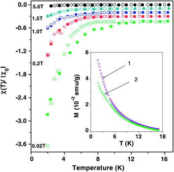 | ||
| Fig. 4 Normalized anisotropic component of the magnetic susceptibility for the aligned 4-Angstrom SWNTs embedded in AFI zeolite crystals. The solid symbols are experimental data and the open symbols are theory. Inset shows the magnetization density of pure AFI crystals (curve 1) and SWNTs@AFI composite (curve 2) under a 2000 Oe magnetic field. Adapted from ref. 15. | ||
2.4. Relevant theoretical studies
The first report of superconductivity in 4 Å SWNTs has stimulated theoretical investigations focused on the competition between superconductivity and Peierls distortion instability in single (3,3) and (5,0) nanotubes, both of which are 4-Angstrom in diameter and metallic in character. A fully ab initio calculation of lattice dynamics and electron–phonon coupling for a (3,3) nanotube was performed with density functional perturbation theory (DFT). Softening of the phonons (q = 2kF) was found with a mean-field Peierls transition temperature of 240 K.30 The authors also used the same method to investigate the electron doping effect on the (3,3) nanotube and found the superconducting tendency to be substantially enhanced with respect to the pristine case.31 However, the Peierls instability still has a higher transition temperature than that of the superconducting transition. Similar results were also obtained by another DFT calculation on the (5,0) nanotube, which found that the increase of the electron–phonon coupling with decreasing radius can lead to a Peierls transition above the room temperature,32 induced by an acoustic long wavelength squashing mode. In contrast, a self-consistent tight binding calculation on the (5,0) nanotube led to the prediction of superconductivity with the consideration of electron–electron Coulomb interaction. In particular, the Peierls transition was found to be suppressed to an unobservable low temperature regime and a superconducting transition temperature of ∼1 K was obtained.33 Through renormalization group calculations, Kamideet al. obtained the phase diagram by calculating the temperature-dependent correlation functions for superconductivity and Peierls distortion in a single (5,0) nanotube. They found the superconductivity to be dominant at low temperatures if the electron–phonon interaction is strong enough.34 The possibility of triplet superconductivity fluctuations was also suggested for the (5,0) nanotube, owing to the specific three-band model35 that is applicable to the (5,0) band structure near the Fermi level.While the above theoretical investigations have focused on the behavior of a single nanotube, Gonzalez and Perfetto considered the dielectric screening effect on the electron–electron Coulomb interaction and the net effective interaction mediated by phonon exchange.36 They showed that the appearance of the strongest relevant instability in the (5,0) nanotube is dependent on the dielectric constant of the environment. Hence the appearance of superconductivity for an array of (5,0) carbon nanotubes, in contrast to that for a single (5,0) nanotube, is potentially possible.
3. A review of intrinsic superconductivity in other carbon nanotube systems
In this section we would like to briefly review the observations of intrinsic superconductivity in other CNTs systems.15,17,18,37,38 In 2001, Kociak et al.17 showed that ropes of single walled carbon nanotubes, about 1.4 nm in diameter, can exhibit superconducting behavior. In one sample an electrical resistance drop at 550 mK was observed, and this drop in resistance can be suppressed by 1 Tesla of magnetic field or 2.5 µA of bias current. The differential resistance versus bias current measurements also showed behaviors in support of superconductivity. The coherence length ξ was estimated to be 300 nm, or ∼10 times the diameter of the SWNTs bundle. It was found that the length L of the SWNTs bundle between two (normal metal) electrodes can affect the superconducting behavior. For a short sample with L ≈ 0.5ξ, no superconducting resistive transition was observed; but when the length of sample was increased to L ≈ 2ξ, superconducting behavior was observed with Tc = 140 mK. For the longest sample with L ≈ 3ξ the superconducting transition temperature was observed to be 550 mK. The proposed explanation for this behavior is attributed to the inverse proximity effect of the normal metal electrodes. Five years later, the same group and their collaborators observed a diamagnetic signal in the purified SWNTs bundles.37 The temperature-dependent diamagnetism was interpreted as the Meissner effect, qualitatively similar to the observation in 4-Angstrom SWNTs.15 The critical temperature from the magnetic measurements is 400 mK, close to the results of electrical transport measurement; and the critical field Hc1 was found to be 60 ± 20 Oe.Nanotube superconductivity was also reported by Takesue et al.,18 with a critical temperature up to 12 K in entirely end-bonded multiwalled carbon nanotubes (MWNTs) encapsulated in nanopores of alumina templates. The outer diameter of the MWNT is about 7.4 nm, while the inner diameter is about 2 nm. It was reported that the junction structure of the Au electrodes/MWNTs is critical to the observation of superconductivity in this system. For partially end-bonded sample, only a small resistance drop was observed below 3.5 K; and no resistance drop was seen for Au-bulk junction sample. This difference was interpreted to arise from the number of electrically active shells, N, of the MWNTs (N = 1 for Au/bulk junction sample, 1 < N < 9 for partially end-bonded sample, and N = 9 for entirely end-bonded sample). It was proposed that the inter-shell electrostatic coupling would suppress the Tomonaga–Lutting liquid state, which competes against the superconductivity.18 The Meissner effect was also observed in honeycomb arrays of these MWNTs (after purifying), manifested as a gradual magnetization drop with an onset temperature of 18–23 K.38 Interestingly, when the alumina template was dissolved and the MWNTs were placed on the Al substrate, the Meissner effect disappeared.38 From this observation, the authors emphasized the importance of the honeycomb structure and the inter-tube coupling for the appearance of superconductivity in this system. The onset temperature of the Meissner effect, 18–23 K, is much higher than the critical temperature of 12 K observed in transport measurements. This discrepancy has been attributed to a larger N that can be achieved in magnetization measurement38 as compared to the transport measurements.
4. New approach to sample synthesis
Although the observation of a Meissner effect constituted a strong indication of superconductivity in 4-Angstrom carbon nanotubes, other aspects of superconductivity, such as the resistive transition and the specific heat anomaly, were not observed at the time owing to the inadequate sample quality. This situation was remedied by a new sample preparation method, described below.As mentioned in Section 2, the synthesis of 4-Angstrom SWNTs involves two steps: growth of the AFI crystals and their subsequent heat treatment. The first step—hydrothermal growth—determines the size, crystallinity and quality of the AFI crystals. The second step—heating treatment—determines the quality and quantity of 4-Angstrom SWNTs formed inside the AFI channels. Both are of equal importance. Jiang et al.39–41 have reported their efforts to optimize the synthesis conditions for growing large and optically clear AFI crystals with good structural integrity. It was found that the incorporation of a bit of silicon into a zeolite framework can give rise to the formation of a negatively charged matrix and Brønsted acid sites, which can play a catalytic role in the formation of SWNTs. Hence the silicon-incorporated AFI crystals have been favorably chosen for the fabrication of 4-Angstrom SWNTs.
In the original approach, the subsequent heat treatment of the AFI crystals was carried out by simply heating the as-made crystals in a vacuum up to 580 °C (as Pyrex tube was used) for several hours. This process has several drawbacks and can lead to low sample quality. First, the CNTs can be formed only by the decomposition of the precursor TPA, but the carbon atoms in the TPA molecules are limited in quantity and cannot fully occupy the channels even if all of them end up forming carbon nanotubes. Second, carbon atoms would inevitably escape from the AFI channels during the TPA decomposition and hence only a fraction would be available to form the CNTs. Third, the N and H atoms from the decomposition of TPA can easily form NH3 molecules, which have a corrosive effect on the AFI crystals.
In order to avoid the shortcomings of the original approach and to increase the filling factor of the CNTs inside the linear pores, we have adopted a new fabrication process in which the AFI crystals are first heated in 300 mbar of oxygen and 700 mbar of nitrogen at 580 °C for 8 hours to remove the precursor, TPA; and then in 300 mbar of ethylene and 700 mbar of nitrogen at the same temperature for the same duration.19 Instead of the original TPA, continuously flowing ethylene gas is externally introduced into the vacated AFI channels as the carbon source to synthesize the 4-Angstrom SWNTs. This approach ensures sufficient carbon source for the formation of CNTs uniformly inside the AFI channels.
The temperature profiles for the old and new fabrication processes are plotted in Fig. 5a and b, respectively. Raman spectroscopy was used to characterize the samples fabricated by the two processes. Typical Raman spectra (red and green lines) are shown in Fig. 5c, obtained with an excitation laser wavelength of 514.5 nm. Two peaks, one at 510 cm−1 and one at 550 cm−1, are noted by arrows. They respectively correspond to the RBM of the (4,2) and (5,0) carbon nanotubes. The magnitude of the RBM, relative to the G-band Raman signal at 1600 cm−1, is an indication for the percentage of carbon in the nanotube form. The inset to Fig. 5c displays a statistical comparison of the outcomes from the two heating processes. The proportion of the 550 cm−1 peak (delineated by green bars) is seen to be ∼10% of the G-band signal, which is significantly higher than the ∼5% average RBM signals observed in samples fabricated by the old process (delineated by red bars).19 An important feature of the statistical result is that for the new process, the RBM/G values are tightly distributed around the average, with no zero values. This is a clear indication of sample uniformity, in contrast to the non-uniformity of the old process in which ∼25% of the samples display no RBM signal or very poor RBM signals.
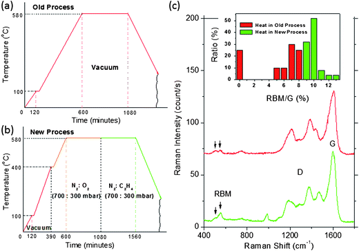 | ||
| Fig. 5 Temperature profiles for (a) the old fabrication process and (b) the new fabrication process. (c) Comparison of the Raman spectra for the old and new processes. Inset shows the proportion of the samples exhibiting the various RBM/G ratios. Fig. 5c is adapted from ref. 19. | ||
While the intensity of the RMB peaks can serve as an indication of the nanotube abundance, the thermal gravimetric analysis (TGA) results, shown in Fig. 6, inform us more accurately the amount of carbon inside the AFI crystal. For the old precursor-conversion approach, TGA results indicate a 1.47 wt% of carbon, whereas the new continuous-carbon-source heating process yields 3.35 wt%. Translated into filling factor for the linear AFI channels, it is 4.5% and 10.3%, respectively, for the two approaches. It should be noted that by using high ethylene pressure (3 atmospheres) at temperatures below 400 °C with subsequent lower ethylene pressure (0.2 atmosphere) at high temperatures (up to 750 °C), we have achieved a maximum of 5.4 wt% carbon. This translates into about 16.6% filling factor in the linear pores. Hence it is important to note that, at best, only a fraction of the AFI zeolite crystals' pores are filled with carbon nanotubes, and among these nanotubes not all of them can be superconducting.
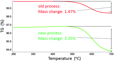 | ||
| Fig. 6 TGA results for the old precursor-conversion approach (red line) and the new continuous carbon source approach (green line). | ||
5. Electrical transport measurements
Very intensive efforts were carried out to clarify the electrical aspect of the superconducting transition. In this section we present only a selection of all the data gathered, for the purpose of illustrating the underlying mechanism. A more inclusive collection of data can be found in ref. 42.5.1. Device fabrication and measurement geometry
According to our early transport measurements,15 the carbon nanotubes inside the AFI crystal channels are likely to be segmented (with length on the order of 100–200 nm). To explore the intrinsic electrical transport property of the carbon nanotubes, a better chance can be afforded by a small separation between the measuring electrodes, on the order of 100 nm. In the following we describe the procedure of device fabrication to make four electrodes on the sample with a separation between the two surface electrodes being ∼100 nm.20The AFI crystals are first heated in 300 mbar of oxygen and 700 mbar N2 at 580 °C for 4 hours, to remove the TPA inside the channels. A selected crystal is picked out and glued on a silicon wafer. Two troughs are etched into the surface of the AFI crystal by focused ion beam (FIB), with a separation of 5 µm. Then the AFI crystal is heated in 300 mbar of ethylene and 700 mbar of nitrogen at 580 °C for 4 hours to form the 4-Angstrom SWNTs inside the linear pores. The AFI crystal (with embedded SWNTs) is subsequently sputtered with 50 nm of Ti as an adhesive layer and 150 nm of Au. The electrical contact geometry is then delineated by using the FIB to remove the Au/Ti film in a predesigned pattern. These processes are followed by vacuum (10−6 Torr) annealing at 450 °C to reduce the contact resistance.
Fig. 7a shows a cartoon picture of the AFI crystal with the four-probe contact geometry, while Fig. 7b shows a scanning electron microscope image of an actual sample. The outer electrodes make end contacts to the SWNTs, whereas the two inner electrodes, each about 2.5 µm wide, are separated by 100 nm and are on the surface of the AFI crystal. We carried out measurements using both the four-probe (with two outer electrodes as the current electrodes) geometry and the two-probe (using only the two surface electrodes) geometry. By using either the current electrodes or the surface electrodes, we have verified that the contacts all display Ohmic behavior. In Fig. 7c and d we show schematically the two-probe geometry and the four-probe measurement geometry, and note that the difference between these two measurement geometries is essentially the transverse resistance, delineated schematically by the dashed circles in Fig. 7c.
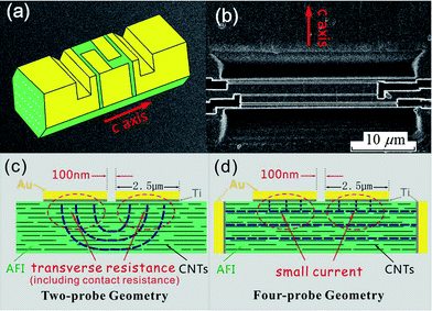 | ||
| Fig. 7 (a) Cartoon picture of the sample. Yellow denotes gold and green denotes the AFI crystal surface exposed by FIB etching. Nanotubes are delineated schematically by open circles. (b) SEM image of one sample. The c-axis is along the N–S direction. The thin, light, horizontal line in the middle is the 100 nm separation between the two surface voltage electrodes that are on its two sides. The dark regions are the grooves cut by the FIB and sputtered with Au/Ti to serve as the end-contact current electrodes. (c) and (d) show schematic drawings of the two-probe and four-probe geometries, respectively. Blue dash lines represent the current paths. In (d), the two end-contact current pads are 4 µm in depth and 30 µm in width. The difference between the two-probe and the four-probe measurements is the transverse resistance, delineated by the red circles in (c). Adapted from ref. 20. | ||
5.2. Quasi one dimensional fluctuation superconductivity
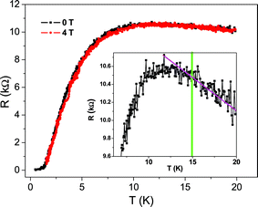
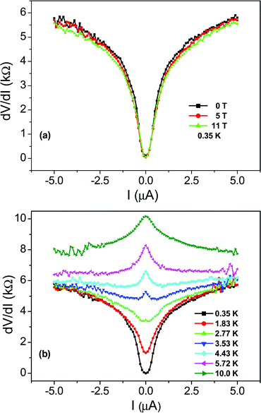
Quasi one dimensional superconductivity was observed in 4-Angstrom carbon nanotubes in 2001, manifest as the Meissner effect. Both the temperature and the magnetic field dependencies of the diamagnetic signal displayed a smooth variation, owing to the fluctuation effect15 (see Appendix B), whereby finite resistance can be generated by thermally activated phase slips as predicted by the LAMH theory43–45 (see Appendix C).Fig. 8 shows the temperature dependence of resistance for sample 1, measured in an Oxford He-3 cryostat. The electrical measurement was carried out in four-probe geometry with a measurement current of 10 nA. It is seen that the resistance decreases smoothly from about 11 kΩ to almost zero, and this behavior does not change under a 4 Tesla magnetic field (applied perpendicular to the c-axis of the SWNTs).19 The inset of Fig. 8 shows an enlarged section between 7 K and 20 K, indicating that the transition initiates at 15 K, consistent with the previous result on the Meissner effect. Fig. 9a shows the differential resistance variation as a function of the bias current at 0.35 K. There is a resistance minimum at zero bias current, a sign of the supercurrent. The resistance increases smoothly with increasing bias current, and this behavior also is not affected by the magnetic field, even up to 11 Tesla. Non-sensitivity to the magnetic field suggests the superconducting component to consist of very thin arrays of nanotubes (with an estimated width of <6 nm), i.e., quasi 1D in character. The smooth resistance variations as a function of temperature/bias current manifestations are consistent with the expected quasi 1D superconductivity behaviors, and they can be interpreted within the framework of thermally activated phase slips as formulated by the LAMH theory.43–45 In this formulation, the wave function ψ = |ψ|exp (iφ) of a superconducting element is regarded to be constant across the cross sectional area (since the cross sectional dimension is smaller than the coherence length) and varies only as a function of x along the c-axis. For a fixed temperature, the magnitude |ψ| is rather rigid and only the phase can change as a function of x. For the periodic boundary condition (such as in the ring geometry), there can only be an integer number n of 2π phase changes, denoted as the winding number. Each winding number n represents a current-carrying meta-stable superconducting state. A larger winding number n corresponds with a higher free energy of the meta-stable state as well as a larger carrying current. Between two neighboring meta-stable states there is always an energy barrier (whose magnitude is proportional to the cross sectional area of the quasi 1D element). As long as the wave function remains in a meta-stable state, the carrying current neither decays nor generates any voltage. That is, the system is still superconducting. However, in the presence of thermal fluctuations, one meta-stable state can transit to another by crossing the energy barrier, and that is the source of the voltage and hence the resistance.
 | ||
| Fig. 8 Temperature dependence of resistance for sample 1. The enlarged section shown in the inset shows the transition begins at 15 K. Adapted from ref. 19. | ||
 | ||
| Fig. 9 The differential resistance plotted as function of bias current for sample 1. In (a), the measurement was done at 0.35 K, showing even an 11 Tesla magnetic field does not change the result. This is an indication that the array must be very thin. (b) While the dip in resistance at low temperature indicates the existence of supercurrent, the zero bias resistance peak above 2.77 K indicates that a competing mechanism (with superconductivity) exists in the system.37 Through second-order renormalization group calculations on thin arrays of (5,0) nanotubes, we interpret it as arising from the existence of Peierls distortion as an excited state. The ground state is singlet superconducting owing to the reduction of Coulomb interaction through dielectric screening by the surrounding nanotubes in the thin array. A single (5,0) tube favors the semiconducting Peierls distortion as the ground state. | ||
Now consider a quasi 1D superconducting element being connected to a current source. Whenever a meta-stable state n transits to a lower free energy meta-stable state n − 1 (which is always more probable than the other way around), the carrying current of the system decreases as well. Since the current source has to maintain the current at a fixed value, it will push the system back up to the meta-stable state n. In this process work is done by the external source, i.e., dissipation has occurred. Another way of saying the same thing is that a voltage will appear as a consequence of the thermally induced transitions between the meta-stable current-carrying states. The magnitude of the voltage is directly proportional to the rate of such transitions.
A mathematical description of the phase slips and the appearance of voltage in a quasi 1D superconductor, based on the LAMH theory, is given in Appendix C.
Fig. 9b shows the bias current dependence of differential resistance at different temperatures. Here we see a very interesting phenomenon in the appearance of a differential resistance peak centered at zero bias current. The peak appears at around 2.77 K, and from the R vs. T behavior the sample should still be in the overall quasi 1D superconducting regime at this temperature. This differential resistance peak clearly indicates that there is a mechanism operating in the system that competes with superconductivity. From recent theoretical work,46 this competing mechanism may be attributed to the Peierls distortion/charge density wave (CDW) (see Appendix B), which behaves as a (higher-energy) excited state while the singlet superconductivity is the ground state of the thin array of (5,0) carbon nanotubes. As the array becomes larger, the energy separation between the Peierls distortion/CDW state and the superconducting ground state would increase, thereby facilitating an eventual transition to the 3D superconducting state as mediated by a Berezinskii–Kosterlitz–Thouless (BKT) transition in the ab plane perpendicular to the c-axis of the nanotubes.20 Such a crossover transition is the subject matter of the following section.
5.3. Crossover from quasi one dimensional to three dimensional superconductivity
A sharp resistive transition is usually taken as the hallmark for bulk superconductivity. However, thermal fluctuations and Peierls distortion (Appendix B) can prevent its occurrence in very thin arrays as we see above. This scenario may change when the size of coherently coupledcarbon nanotube arrays increases, and indeed a crossover from quasi one dimensional to three dimensional superconductivity has been observed as shown below. In particular, this crossover involves a BKT-like transition in the ab plane of the aligned nanotube arrays. We use “BKT-like” to describe the transition because the BKT transition is strictly a 2D transition, whereas here the third dimension (along the c-axis) definitely participates in the transition. Nevertheless, we shall show that the sharp resistance drop observed, concurrent with the appearance of nonlinear I–V behavior, is in very good agreement with the predicted manifestations of a BKT transition.Fig. 10a shows the temperature dependence of resistance for sample 2, measured with two-probe geometry (i.e., using the two surface electrodes) in the Quantum Design Physical Property Measurement System. A sharp drop is seen to initiate at 7.5 K, and this drop is moved to lower temperatures with increasing magnetic fields, applied perpendicular to the c-axis.20 The fact that a magnetic field can affect the transition temperature means that the superconductivity originates from coupled carbon nanotube arrays which must extend at least a few tens of nanometres in the transverse dimension. The inset of Fig. 10a shows the enlarged upper section of the curves from 3 K to 20 K, with the straight line above 17 K subtracted. The appearance of the magnetoresistance clearly shows that the superconducting transition starts at 15 K, consistent with the previous data. The magenta curve in the bottom of Fig. 10a is the four-probe data measured at zero field. It is seen that the difference between the four-probe resistance and the two-probe resistance almost disappears below 5 K, i.e., the transverse resistance is almost zero below 5 K.
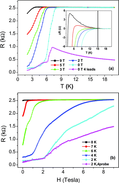 | ||
| Fig. 10 (a) Temperature dependence of resistance for sample 2, measured with 1 µA current. The magenta curve is the four-probe data and the others are two-probe data. Inset is a magnified view of the upper section from 3 K to 20 K with the straight line asymptote above 17 K subtracted, indicating the superconducting transition initiates at 15 K. Between 15 K and 7.5 K the finite resistance is due to the phase-slips in independently fluctuating quasi-1D superconductors. 1D to 3D crossover transition occurs at 6–7.5 K, via establishing phase coherence in the plane perpendicular to the c-axis of the aligned nanotubes, concurrent with the quenching of the long wavelength fluctuations along the c-axis. (b) MR of sample 2 under different temperatures, with magenta curve being the four-probe data and others being the two-probe data. In both (a) and (b) it is important to note that the 4-probe data coincide with the two-probe data below 6 K and 2.1 Tesla. This is an indication that the transverse resistance in this sample has nearly vanished (see Fig. 7c and d for the difference between the 4-probe and 2-probe measurements). Adapted from ref. 20. | ||
Fig. 10b shows the magneto-resistance in sample 2, which is strongly temperature dependent. At 2 K, there is a clear transition point at 2.1 Tesla, below which the difference between the four-probe resistance and the two-probe resistance disappears. Thus the transverse resistance can be turned on/off by varying either the temperature or the magnetic field.
5.4 Physical interpretation
For the resistance drop initiating at 7.5 K, which is concurrent with the transverse resistance becoming zero below a certain temperature/magnetic field, our interpretation is that it is due to a BKT-like transition in the transverse ab plane.We consider our carbon nanotube arrays to comprise quasi 1D superconducting elements. For simplicity, we model these elements to form a close-packed triangular lattice as illustrated by the dots in Fig. 11. Each element is characterized by a complex Ginzburg–Landau wave function47ψ that is a function of x along the c-axis. Starting at 15 K, the formation of superconducting condensate in the nanotubes is responsible for the magneto-resistance seen in the inset of Fig. 10a. Owing to the quasi one dimensionality of the superconducting element, strong long wavelength thermal fluctuations prevent the appearance of a sharp superconducting transition in individual elements. However, when the temperature is lowered, the growth of the superconducting condensate would increase the Josephson constant J (see below), which favors the enhanced transverse coupling between the neighboring elements. The Josephson interaction energy between two neighboring quasi 1D elements is defined as −Jcos (φi − φj), where φi denotes the phase of the wave function of the ith element, assumed to be a constant over the longitudinal coherence length along the c-axis, with J being proportional to the superconducting electron density |ψ|2 as well as to the overlap of the aligned neighboring nanotubes along the c-axis direction. Since the Josephson coupling can be alternatively written as −J(![[S with combining right harpoon above (vector)]](https://www.rsc.org/images/entities/b_i_char_0053_20d1.gif) i·j), where i denotes a unit vector in the transverse ab plane, our system is analogous to a 2D XY spin model in which it is well known that there can be vortex excitations, consisting of spins that form a closed loop as shown in Fig. 11. Moving vortices will destroy coherence in the transverse plane. However, vortices of opposite helicities interact as attractive 2D charges with a logarithmic potential. They can become bound pairs at a BKT transition temperature, below which one expects the establishment of transverse coherence in the ab plane48,49 whereby the phase coherence decays only as a power law (as opposed to decaying exponentially) of the transverse separation (between two elements) in the ab plane. This is usually denoted as quasi long range order. The establishment of phase coherence in the ab plane would quench the longitudinal fluctuations since the transverse cross section effectively becomes much larger and hence the energy barrier for phase slips increases dramatically. Therefore the resistance in the 4-probe resistance (magenta curve in Fig. 10a) is seen to experience a sudden drop. However the resistance is not zero below the BKT-like transition. The interpretation is that we have 3D superconducting regions separated by weak links. Here the term “weak links” is meant to denote the Josephson junctions along the c-axis caused by defects or imperfections of the nanotubes. Their existence can be the main cause of the non-metallic temperature dependence of the 4-probe resistance data above the BKT-like transition (see the magenta curve in Fig. 10a). However, these weak links would successively turn superconducting below 5 K as seen below, so that at 2 K global coherence is attained.
i·j), where i denotes a unit vector in the transverse ab plane, our system is analogous to a 2D XY spin model in which it is well known that there can be vortex excitations, consisting of spins that form a closed loop as shown in Fig. 11. Moving vortices will destroy coherence in the transverse plane. However, vortices of opposite helicities interact as attractive 2D charges with a logarithmic potential. They can become bound pairs at a BKT transition temperature, below which one expects the establishment of transverse coherence in the ab plane48,49 whereby the phase coherence decays only as a power law (as opposed to decaying exponentially) of the transverse separation (between two elements) in the ab plane. This is usually denoted as quasi long range order. The establishment of phase coherence in the ab plane would quench the longitudinal fluctuations since the transverse cross section effectively becomes much larger and hence the energy barrier for phase slips increases dramatically. Therefore the resistance in the 4-probe resistance (magenta curve in Fig. 10a) is seen to experience a sudden drop. However the resistance is not zero below the BKT-like transition. The interpretation is that we have 3D superconducting regions separated by weak links. Here the term “weak links” is meant to denote the Josephson junctions along the c-axis caused by defects or imperfections of the nanotubes. Their existence can be the main cause of the non-metallic temperature dependence of the 4-probe resistance data above the BKT-like transition (see the magenta curve in Fig. 10a). However, these weak links would successively turn superconducting below 5 K as seen below, so that at 2 K global coherence is attained.
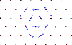 | ||
| Fig. 11 A schematic picture of the transverse plane perpendicular to the c-axis, with each dot representing an end-view of a segment of the 1D superconducting nanotubes. A vortex excitation, indicated by arrows whose directions are given by the phase (angles) of the 1D wavefunction, is shown. Interaction between a clockwise vortex and counter-clockwise vortex is long-range in character, thereby facilitating a transition that can establish quasi long range order (meaning that the correlation decays as a power law) in the ab plane (perpendicular to the c-axis) of the nanotube arrays. Adapted from ref. 20. | ||
In the above model, the quasi 1D elements may be viewed as regions of relative homogeneity in which the neighboring nanotubes have significant overlaps along the c-axis direction and hence a larger value of J. The Josephson junctions between the quasi 1D elements are regions where the overlaps between neighboring nanotubes are small, thus leading to much weaker coupling than that within the quasi 1D elements. Hence the model inherently belongs to the class of inhomogeneous superconducting systems.
The effect of the magnetic field is mainly due to its influence on J through the suppression of superconducting electron density within the quasi 1D elements, which has the effect of both shifting TBKT to lower temperatures and diminishing the magnitude of the resistance drop associated with the transition. This aspect differs from the traditional BKT transition's magnetic field effects, since here the magnitude of J is controlled by the condensate along the c-axis.
A BKT transition is usually characterized by two aspects: (1) the nonlinear I–V behavior below a BKT mean field transition temperature TC0,50,51 and (2) the special temperature dependence of resistance above the BKT transition temperature TBKT < TC0.49,52 Our interpretation of the 1D to 3D crossover as a BKT transition, in the transverse ab plane, is supported by measured data in both accounts.
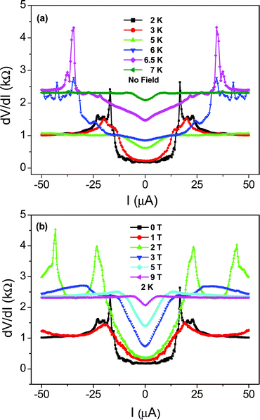 | ||
| Fig. 12 Bias current dependence of differential resistance for sample 2 measured in two-probe geometry. The magnetic field is perpendicular to the c-axis of the SWNTs. Adapted from ref. 20. | ||
Below the BKT transition temperature, the system comprises 3D superconducting regions connected by weak links, and the second plateau (1 kΩ) corresponds to the resistance of the weak links in the normal state. When the temperature further decreases to 2 K, the weak links become superconducting, and global coherence is attained as identified by the well-defined supercurrent gap.
Fig. 12b shows the data measured at 2 K under various perpendicular magnetic fields. The general behavior is seen to be similar to those shown in Fig. 12a. This similarity means that the applied magnetic field may be viewed as having the effect of decreasing the transition temperature. The two plateaus and their associated gaps are clear indications of the progressive establishment of coherence within the system.
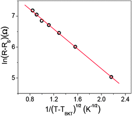 | ||
| Fig. 13 Theoretical fitting according to ln (R − RS) ∝ (T − TBKT)−1/2 at T > TBKT for zero field data of sample 2. RS = 1.06 kΩ is the lower plateau resistance shown in Fig. 12, which arises from the weak links connecting different superconducting regions along the c-axis. Adapted from ref. 20. | ||
Due to the 1D nature of carbon nanotubes, there should be some anisotropy in our system. Fig. 14a shows the temperature dependence of resistance for sample 3, which was measured with three probes, as one current lead was (unintentionally) short circuited to its neighboring voltage lead. Similar behavior to sample 2 is seen, though the resistance is much smaller. The temperature dependence of the transition is noted to also follow the ln (R − RS) ∝ (T − TBKT)−1/2 behavior20 with a TBKT = 5.9 K.
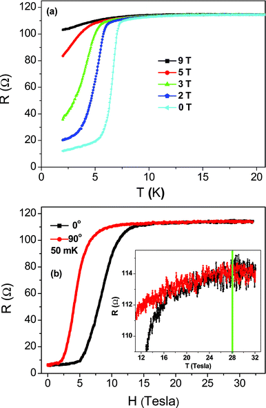 | ||
| Fig. 14 (a) The temperature dependence of resistance for sample 3, measured with three-probe configuration. It is shown in ref. 20 that the temperature dependence of the transition also follows the ln (R − RS) ∝ (T − TBKT)−1/2 behavior, with a TBKT = 5.9 K. (b) MR anisotropy measured at 50 mK, with magnetic field being parallel (0°) and perpendicular (90°) to the c-axis of carbon nanotubes. Inset shows the enlarged section of the high magnetic field part. It is seen that the anisotropy disappears above 18 Tesla, but positive MR is maintained until 28 Tesla. Adapted from ref. 20. | ||
Shown in Fig. 14b are the magneto-resistance results under both the perpendicular and parallel magnetic fields, measured at 50 mK in the Grenoble High Magnetic Field Laboratory, France. The magnetic anisotropy is evidenced by the clear lateral separation of the two curves, with the magnetic field perpendicular to the c-axis being more effective to suppress superconductivity than the same field applied parallel to the c-axis. Similar to sample 2, the magneto-resistance displays an S-shape, with the first turning point at 2 Tesla and 5 Tesla for the perpendicular and parallel fields, respectively, and the second turning point at 10 Tesla and 13.5 Tesla. The resistance increase between these two turning points is attributable to a decrease in the ab plane coherence, accompanied by an increase in longitudinal fluctuations. Hence the system is basically reduced to quasi-1D after the second turning point. If we take the 5 Tesla and 13.5 Tesla as the lower and upper bounds of the parallel critical field for the 3D superconducting phase, then the coherence length may be estimated as ξab = (Φ0/2πHc‖)1/2 ≈ 5 to 8 nm in the ab plane. Here Φ0 = 2.07 × 10⁻⁷ G cm2 is the quantum flux. In a similar manner, the coherence length ξc along the c-axis may be estimated to be ∼7 to 12 nm.
The anisotropy disappears above 18 Tesla, which may imply the suppression of the superconducting condensate in individual nanotubes, i.e. the Pauli limit. However, the resistance keeps increasing until 28 Tesla as seen in the inset of Fig. 14b. This may indicate an FFLO state in our system. As predicted by P. Fulde, R.A. Ferrell, A.I. Larkin and Y.N. Ovchinnikov,53,54 when approaching the Pauli limit, type-II superconductors have the possibility of increasing their upper critical fields by “sacrificing” a part of their volume to the normal state in the form of a spatial modulation of the superconducting order parameter. Such a state can only be realized in low-dimensional superconductors as it requires an open Fermi surface in order to increase the orbital limit for superconductivity beyond the Pauli limit.55,56 In this sense our quasi one-dimensional superconductor fulfills the necessary requirements.
In Fig. 15 we plot the magnetic field-temperature phase diagram for our system, with the experimental data of sample 2 and sample 3. Here yellow denotes the 1D fluctuating superconductor regime, the green line denotes the TC0 variation and the blue line denotes the TBKT variation, both associated with the BKT transition. The area colored by violet is the regime where one expects to see nonlinear I–V characteristics. Green is the regime in which the sample is characterized by inhomogeneous 3D superconducting regions connected by normal weak links. The bottom left corner is the regime of global coherence. Here, symbols are the data, with the connecting solid lines used to delineate the different regimes. The symbols on the vertical axis mark the positions of the first turning point, the second turning point and the merging point obtained from the measurements on sample 3 at 50 mK. The solid symbols are for the perpendicular case and the open symbols are for the parallel case. The triangular region on the upper left corner denotes the FFLO state as discussed above.
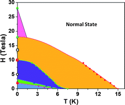 | ||
| Fig. 15 Magnetic field-temperature phase diagram summarized from the experimental data for samples 2 and 3. Here yellow, violet, green and blue regions denote, respectively, the fluctuating 1D superconducting regime, the nonlinear I–V regime, the regime in which the 3D superconducting regions are connected by weak links, and the global coherence regime. The solid symbols of circle, square and triangle on the vertical axis denote the demarcation points as measured by a perpendicular magnetic field at 50 mK for sample 3. The open symbols are the corresponding points measured by a parallel field. The triangular region on the upper left denotes the FFLO state that is to be further verified. Adapted from ref. 20. | ||
6. Magnetic Meissner effect
Besides the observation of superconducting resistive transition, the detection of diamagnetic screening from the (fluctuations) magnetic Meissner effect is generally regarded as one of the definitive probes of superconductivity. In 2001, we reported an early observation of the magnetic Meissner effect in 4-Angstrom SWNTs embedded in AFI crystals.15 A smooth-varying (anisotropic) diamagnetic signal was reported below ∼15 K. These early samples had very low (nanotube) filling factors of the AFI pores which made a quantitative investigation of the Meissner effect difficult. In the meantime, the sample quality has been improved as described in Section 4 and a filling factor (in the linear pores of AFI zeolite) of up to 10% has been achieved. In 2011, we reported new and far more detailed magnetic experiments on such samples measured in two totally different ways—using a SQUID VSM magnetometer and the magnetic torque approach21—with consistent results.6.1. Bulk magnetization measurements
Even with the new samples, the volume fraction of the CNTs in the AFI host is still tiny. Any magnetic signal is therefore largely dominated by paramagnetic and diamagnetic contributions from the AFI host. The bulk magnetization of new samples has been measured with a SQUID VSM magnetometer. The upper left inset of Fig. 16 shows a typical magnetization measurement as a function of the magnetic field at 1.8 K. The data display the typical S-shape of a paramagnetic Brillouin function, which is superimposed on the linear diamagnetic contribution with a negative slope. Resolving the superconducting contribution requires zooming in onto the low field region as presented in the main graph. A tiny feature is visible in small magnetic fields, which shows the characteristics of a superconductor in the vicinity of the lower critical Hc1 transition. The initial zero-field cooled (ZFC) curve starts with a linear field dependence of negative slope representative for the Meissner state. At ∼60 Oe the curve deviates from linearity, which may be interpreted as the Hc1 point. Beyond that, the magnetization passes through a sharp minimum and then turns up. A hysteresis is found for the following branches of the magnetization loop which indicates pinning of the magnetic flux. The lower right inset shows similar data for another sample with stronger flux pinning but a similar initial ZFC curve.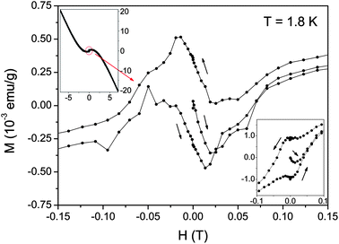 | ||
| Fig. 16 Upper left inset: full magnetization loop of 4 Angstrom carbon nanotubes embedded in AFI crystals measured at T = 1.8 K. The circle encloses a tiny anomaly at Hc1. Main graph: Enlargement of the encircled area in the inset in small fields around the superconducting Hc1 transition. Lower right inset: similar data as in the main graph for a second sample with stronger flux pinning. The field has been applied perpendicular to the c-axis of the CNTs. Adapted from ref. 21. | ||
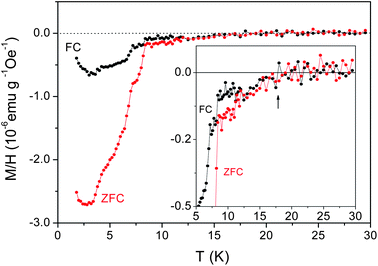
Fig. 17 shows a temperature-dependent magnetization measurement in a field of 20 Oe under ZFC and field-cooled (FC) conditions. A sharp onset of a strong diamagnetic signal is found slightly above 7 K. At the same temperature the ZFC and FC branches strongly deviate from each other. The inset shows an enlargement of the data to illustrate that the onset of the diamagnetic Meissner effect occurs at ∼18 K and irreversibility due to flux pinning starts to become significant below ∼12 K. The sharp feature at 7 K, which is well separated from the onset of the diamagnetic signal, indicates that the superconductivity occurs in several stages. Below 18 K superconducting fluctuations start to form. This coincides well with the temperature below which a downturn has been observed in the resistivity, as described in Section 5.3. Hence this sharp feature at 7 K may represent the bulk superconducting transition, below which 3D macroscopic phase coherence is formed. This sharp feature fades away rather quickly in higher fields21 and the superconducting signal becomes hidden in the rapidly growing paramagnetic contribution.
 | ||
| Fig. 17 Temperature dependence of the zero-field cooled (ZFC) and field cooled (FC) magnetization in a magnetic field of 20 Oe applied perpendicular to the c-axis of the CNTs. The inset shows an enlargement of the data at higher temperatures in order to point out the onset of a diamagnetic signal at ∼18 K. Here the mass normalization (for obtaining the M/H values) is done by using the total mass of the sample. Adapted from ref. 21. | ||
Some geometric information about the sample may be deduced from the data shown in Fig. 17. By using the TGA data that indicate the carbon content of the sample to be ∼3.35 wt% (see Fig. 6) and the fact that the carbon density inside the linear channels (taking into account the channel–channel separation) is 0.585 g cm−3, we obtain from the ZFC data at 2.5 K a dimensionless magnetic susceptibility χ = −4.36 × 10⁻⁵. Since χ ≅ −(0.125)(w/λ)2 for an array with a (transverse) diameter w and magnetic penetration length λ ≫ w in a parallel magnetic field, we estimate that w ≈ 25 nm if λ = 1.5 µm (see below). This estimate ignores the difference between a parallel and perpendicular field (since the data is for perpendicular field) and therefore can only afford a rough value. Nevertheless, this value of w compares reasonably with similar values deduced from transport measurements,20 ranging from 36 nm to 57 nm, obtained from different samples.
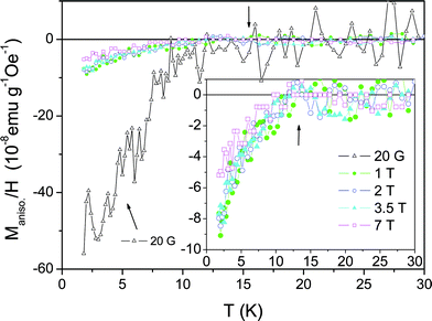
Further information about superconductivity in higher applied fields can be extracted from the anisotropic component of the magnetization. Due to the 1D nature of the CNTs, at least some anisotropy in the superconducting signal is expected. On the other hand, the paramagnetic and diamagnetic background should be largely isotropic. In Fig. 18 we plot the difference Mpar. − Mperp. of the magnetization data measured in fields applied once parallel to the c-axis of the CNTs and once perpendicular. The derived data is basically zero at temperatures above 15 K. For temperatures below 15 K, a negative signal is observed which means that a magnetization signal of larger magnitude for parallel applied fields develops. The signal indicates the presence of superconducting correlations which exist up to magnetic fields well beyond our maximum available field of 7 Tesla, in accordance with our resistivity data in Section 5. The negative signal of an anisotropic component is consistent with the result of magnetic torque measurements in the same batch of sample (see section 6.2),21 but is different from the result of the old Meissner effect result in 2001.15 The difference comes from the filling factor of carbon inside the AFI channels, as 1D fluctuation superconductivity dominated in the old samples, but 1D to 3D superconductivity crossover occurred in the new samples with increased filling factor.21 From the electrical transport results in Section 5.3, we know that the 3D bulk superconductivity is established below the BKT transition. And below the BKT transition temperature, the macroscopic screening currents can flow freely in the sample and the long hexagonal c-axis of the AFI crystals will have a strong tendency to align parallel to the applied magnetic field in order to reduce the demagnetization factor, resulting in a larger magnetization parallel to the c-axis. The anisotropic signal is seen to be much smaller at fields above 1 Tesla. But the negative sign of the anisotropic magnetization, at 7 Tesla, shows that some bulk coherence may still persist if the field is parallel to the c-axis, but absent if the field is perpendicular. This is consistent with the anisotropic magnetoresistance result shown in Fig. 14b. A more detailed discussion can be found in ref. 21.
 | ||
| Fig. 18 Temperature dependence of the anisotropic component of the magnetization, derived from the difference in the measured magnetizations with magnetic fields applied parallel and perpendicular to the c-axis of the CNTs. The inset shows the high magnetic field regime in more detail. Adapted from ref. 21. | ||
6.2. Magnetic torque measurements
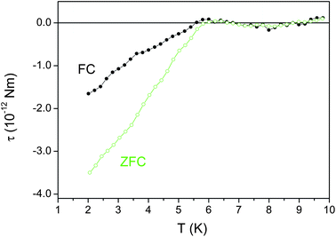
The magnetic torque is defined as τ = M × H, where M is the anisotropic component of the magnetization and H is the applied magnetic field. The anisotropic magnetization can rule out the effect of isotropic magnetic impurity effects in the sample, which should yield no magnetic torque. The magnetic torque was measured with a homemade capacitive cantilever as described with some detail in ref. 21. The samples and the cantilever were aligned in a way that the c-axis of the CNTs was oriented at 45 degrees with respect to the magnetic field to ensure a large signal.21Fig. 19 shows the temperature dependence of the magnetic torque which was zero-field cooled (ZFC) or field-cooled (FC) with a magnetic field of 100 Oe. The magnetic torque changes from zero to a negative value at around 6 K, and the FC/ZFC curves deviate from each other below 6 K. The negative value of the magnetic torque is consistent with the bulk anisotropic magnetization measurement shown in Section 6.1, and is a signature that the 3D phase-coherent superconductivity is established in the sample. The larger magnitude of the ZFC data further proves the existence of the macroscopic superconducting screening currents which can only flow in a bulk superconducting state and not in individually uncoupled 1D SWNTs with superconducting fluctuations. Fluctuation superconductivity up to 15 K is not observed in this measurement, mainly due to the experimental limitation of the magnetic torque approach that is essentially set by the drift of the capacitance measurement.
 | ||
| Fig. 19 ZFC and FC curves of the magnetic torque for 4-Angstrom carbon nanotubes in a field of 100 Oe. Adapted from ref. 21. | ||
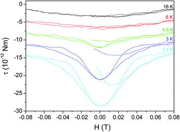
The magnetic torque variation at small magnetic fields is shown in Fig. 20 for different temperatures. While the magnetic torque shows a very weak field dependence above 16 K, the reduction of the torque signal begins to appear at temperatures below 6 K in fields smaller than 0.4 Tesla, and it becomes very pronounced at 1.7 K. These data exhibit the typical behavior of the reversible magnetization of a superconductor close to the lower critical field Hc1, which is ∼60 Oe in this case. This value is noted to be on the same order as the 60–150 Oe measured by using the SQUID VSM, shown in Fig. 16.
 | ||
| Fig. 20 The magnetic field dependence of the magnetic torque at different temperatures. The curves have been shifted for clarity. Adapted from ref. 21. | ||
If we take Hc1 ≈ 60 Oe, then the magnetic penetration length λ can be estimated from the formula 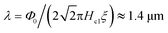 , provided ξ ≈ 18 nm as estimated from the Hc2 ≈ 1 T in Fig. 18. That means the Ginzburg–Landau κ = λ/ξ ≈ 78.
7. Thermal specific heat characteristics
The observation of the superconducting transition in the specific heat of 4-Angstrom SWNTs embedded in AFI crystals has been reported in 2009.19 As a measurement of the heat capacity probes the entire volume of the sample, the detection of the characteristic specific-heat anomaly associated with the superconducting transition is considered a definitive bulk proof of superconductivity. The embedded CNTs represent only a tiny volume fraction of the composite material. Therefore, the signal is largely dominated by phonon contributions from the AFI zeolite. The detection of the tiny superconducting signal certainly pushes the available techniques to the limit of resolution. To overcome this difficulty, we developed an ultra-high resolution AC modulated temperature calorimeter.57 A stimulated periodic modulation of the sample temperature is detected with a long integration time by means of a digital lock-in amplifier, which, together with a low-noise transformer, allows us to determine changes in the heat capacity with sufficiently high resolution.The upper left inset of Fig. 21 shows the total specific heat divided by temperature C/T of CNT@AFI, which is on first view a smooth function without visible anomaly. Resolving the superconducting transition requires careful subtraction of the phonon contributions from the zeolite and the SWNTs. This is typically done by applying a sufficiently high magnetic field to suppress the superconductivity. As any available temperature sensor shows certain magnetic field dependence at cryogenic temperatures, a very precise calibration of the thermocouple temperature sensor was needed in order to obtain sufficient accuracy. We have chosen a field of 5 Tesla as reference data, partly due to technical limitations related to the fact that the precision of the field calibration is strongly reduced in higher magnetic fields. In the main graph of Fig. 21 we present the so-obtained electronic contribution to C/T for various magnetic fields. A broad second-order jump appears with a peak at ∼11 K and onset at ∼15 K. At higher temperatures C/T reaches a constant value, which typically represents the Sommerfeld constant (∼3 µJ g−1K−2). At the lowest temperature C/T approaches zero. This indicates a complete development of a superconducting gap. The vanishing slope of C/T at lowest temperatures reflects the absence of nodal lines in an order parameter of s-wave symmetry. The overall shape resembles a strongly broadened BCS curve. Details of the superconducting parameters that can be obtained from the zero field data are discussed in the relevant reference.19 The values obtained for the coherence length ξ and magnetic penetration length λ are 14 nm and 1.5 µm, respectively. They are noted to be consistent with those deduced from the electrical and magnetic measurements, given in Sections 5 and 6.
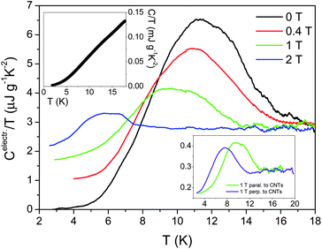 | ||
| Fig. 21 Upper left inset: total specific heat C/T of 4 Angstrom carbon nanotubes embedded in the linear channels of AFI zeolite. Main graph: Electronic contribution to the specific heat of 4 Angstrom carbon nanotubes embedded in the linear channels of AFI zeolite measured in magnetic fields of 0, 0.4, 1 and 2 Tesla. The magnetic field has been applied perpendicular to the c-axis of the nanotubes. Data measured in 5 Tesla have been used to separate the dominant phonon background contribution, which arises mostly from the zeolite. Lower right inset: specific heat measured in 1 Tesla for a magnetic field applied perpendicular and parallel to the c-axis of the nanotubes, illustrating that only a small anisotropy is found in magnetic fields. Adapted from ref. 19. | ||
In a magnetic field, the superconducting anomaly shown in Fig. 21 is quickly suppressed as though a magnetic field of 5 Tesla would be indeed sufficient to fully restore the metallic state. From resistivity measurements in Section 5.3 we know however that a field of 5 Tesla basically only suppresses macroscopic phase coherence of the superconducting condensate. Superconducting correlations are present up to a much higher field of 28 Tesla.20
The specific heat anomaly seen in Fig. 21 most likely represents only a part of the total superconducting specific-heat signal, related to a growing superconducting condensate competing with a decreasing correlation length as the temperature is lowered. This anomaly can be reproduced by simulations using the Ginzburg–Landau phenomenological theory, coupled with the BCS specific heat expression.19 The lower right inset of Fig. 21 illustrates that the direction of the applied magnetic field of 1 Tesla (parallel and perpendicular to the c-axis of the SWNTs) has only a comparatively small effect on superconductivity. These correlations are therefore largely 3D in nature and should, at least partly, represent short-range correlations between parallel SWNTs. However, in recent simulations the BKT-like transition in the ab plane of the nanotube arrays is seen to contribute only a very small specific heat anomaly, ∼1/100 the size of the main peak, just above the BKT transition temperature. This is owing to the small entropy change associated with the establishment of quasi long range phase coherence in the ab plane. Therefore the main contribution of the specific heat anomaly arises from the thermal fluctuations of the magnitude of the Ginzburg–Landau wavefunction |ψ| (which is only marginally affected by fluctuations and the accompanying phase slips below 15 K), instead of the transverse coherence in the ab plane. That also explains why the peak appears at a temperature higher than the BKT transition temperature, which signals the transition to 3D superconductivity.
A possible further contribution to the specific heat, which is not observed when data in which only 5 Tesla was used to separate the background, may be related to the formation of individual Cooper pairs. Much higher fields would be required to suppress their formation. This intriguing possibility stimulates possible further measurements in higher magnetic fields to clearly identify the different contributions to the specific heat. Due to the expected small signal and the required high magnetic fields of up to 28 Tesla, this is however a difficult task.
8. Concluding remarks
In this section we would like to address, in view of the results presented above, some of the issues that have often been raised regarding the superconductivity in our nanotube system. This will be followed by stating some of the challenges and future prospects.Issue 1: can the observed superconductivity be a result of doping?
The likelihood of unintentional doping is very small because a consistent transition temperature, e.g., 15 K (where the magnetoresistance begins to appear), has been observed in different sample batches fabricated via different methods over a period of years. Unintentional doping simply cannot possibly achieve such consistency. Doping by nitrogen (from the AFI zeolite precursor tripropylamine) during the synthesis of SWNTs can also be excluded, since we have observed superconductivity in samples synthesized with pure ethylene.Issue 2: can the observed superconductivity be the result of some type of proximity effect?
This may be excluded because bulk measurements, i.e., magnetic and thermal specific heat measurements, do not involve any electrode contact and yet they have yielded data that are consistent with the electrical measurements.Another reason for excluding the proximity effect is that the most consistently observed initiating temperature—15 K—is higher than the critical temperature of most of the superconductors one may use as an electrode.
Issue 3: what is the role of the zeolite template in the observed superconductivity? Why can't the nanotubes be taken out of the zeolite template so that the superconductivity is directly observed on the nanotubes alone, without the template?
Beyond the physical regulation of the nanotube separation, the effect of the zeolite matrix on the electronic characteristics has been examined through density functional theory calculations and shown to be relatively minor.58 We have tried to measure the properties of the free-standing carbon nanotubes by dissolving the zeolite template. However, the free-standing 4-Angstrom carbon nanotubes were not stable. This fact was also seen during previous HRTEM and Raman measurements. Another concern is that there will be more defects in the carbon nanotubes when they are released from the zeolite template.Issue 4: is the observed superconductivity the BCS type?
The specific heat results can be fitted by the Ginzburg–Landau phenomenological theory, coupled with the BCS specific heat expression. However, more experiments (such as isotopic effect, scanning tunneling microscope measurements) are needed in order to pin it down.Issue 5: if the 4-Angstrom carbon nanotubes are superconducting, there is no reason why it is the only type that is superconducting. Is there evidence for superconductivity in other nanotube systems?
This is a very good point. It is noted that superconductivity has been reported by other groups.16–18 In our group, we have also observed superconductivity in double-walled carbon nanotube bundles. Report on this aspect of our endeavor is forthcoming.Issue 6: in Fig. 9(b), isn't the differential resistance peak that appears above 2.5 K a manifestation of the Luttinger liquid behavior?
Luttinger liquid generally applies to the armchair (n,n) carbon nanotubes. For the (5,0) nanotubes, there are three bands that cross the Fermi level. This feature implies that it cannot be completely similar to the Luttinger liquid behavior. Moreover, the Luttinger liquid model may break down in ultra-thin carbon nanotubes,59,60 because in the presence of phonon-mediated electron–electron interaction the system may deviate from the Luttinger fixed point if the net effective interaction is attractive and would thereby scale to the strong coupling limit.Issue 7: what is the value of the Josephson coupling constant J?
From the relation kBTBKT = πJ/1.12 and TBKT = 6.2 K, we obtain J = 0.19 meV. It should be noted that J is proportional to the average length of linear overlap between the nearest-neighbor nanotubes. Hence for small overlap or for a small segment region along the c-axis, the value of J can be considerably smaller.Issue 8: since the BKT-like transition occurs in the ab plane, why can't it be detected by measuring across the two sides of an AFI crystal?
In principle, this would be the most direct way to detect the BKT-like transition, provided the carbon nanotube content is sufficient so that there can be a percolating network in the ab plane, linking the two sides of the AFI crystal. Unfortunately, at present the samples are still far from percolating. We have actually tried to measure the transition across an AFI crystal, but found only insulating behavior. However, by thinning down the sample to within a typical “connected feature” size in the ab plane, it is entirely possible that such an experiment can succeed. A plan along this direction is already under way.Challenges
While the fact that the 4-Angstrom SWNTs can be superconducting is beyond reasonable doubt, it remains a challenge to achieve 100% consistency in the fabrication of samples that exhibit superconductivity. Consistency in that regard would require further improvements on sample quality as determined by the nanotube filling ratio in the zeolite pores, as well as in the continuity and length of the 4-Angstrom carbon nanotubes. Basic to the sample quality is the control on both the AFI crystal growth and the SWNTs synthesis through the decomposition of the carbon source(s). Making reliable electrical contacts to the sample represents another challenge, as well as the theoretical understanding of the observed phenomena that would require physical insights supported by both microscopic first principles calculations as well as phenomenological modeling.Prospects
The confirmation of superconducting phenomena in carbon nanotubes makes it imperative to further understand the microscopic nature of the observed superconducting phenomena. Thus the isotope effect, the direct observation of superconducting gap through STM measurements, the removal of the AFI matrix, the chemical doping or electrical gate doping effect on the transition temperature, as well as the high pressure effect, etc., are the tasks to be actively pursued. Among them, perhaps the most exciting is the prospect of doping the (5,0) nanotubes by either chemical means or gate voltage. This is because the band structure of the (5,0) nanotube is such that through doping, a significant increase is possible for the Fermi-level density of states, and this is envisioned to significantly enhance the transition temperature since the Debye temperature of carbon is among the highest of all the elements.Appendix A
Superconducting parameters
| Transport measurement | Magnetic measurement | Specific heat measurement | |
|---|---|---|---|
| T c | 15 K | 15–18 K | 14–18 K (exp.), 15 K (best fit) |
| T BKT | 6.2 K | 6–7 K | — |
| H c1 for the Meissner state | — | ∼60 to 150 Oe | ∼100 ± 50 Oe |
| H c2 for the 3D coherent state | H c2⊥ = 1.5–5 T, Hc2∥ = 5–13 T | H c2⊥ ≈ 1 T | H c2⊥ ≈ 2.8 T |
| ξ 0 |
ξ
ab
≈ 5 to 8 nm,
ξ c ≈ 6.6 to 12 nm |
∼18 nm | 14 ± 2 nm |
| λ | — | ∼1.4 µm | 1.5 ± 0.7 µm |
| κ | — | ∼78 | ∼110 |
T c: the critical temperature at which the superconducting condensate begins to form along the c-axis of the carbon nanotubes. For magnetization and specific heat measurements, the superconducting condensate fluctuations were observed to appear at 18 K.
T BKT: the BKT transition temperature, below which there can be coherent 3D superconducting regions. Specific heat associated with the BKT transition is too small to be detected.
H c1: the lower critical field at which the magnetic field first penetrates into the superconducting region.
H c2: the upper critical field at which the 3D coherent superconducting state is suppressed.
ξ 0: the zero temperature coherence length that characterizes the size of the Cooper pairs.
λ: the magnetic (London) penetration depth. The very large value of λ is due to the porous nature of our superconducting system.
κ: defined as κ = λ/ξ. κ ≈ 100 signifies our 4-Angstrom carbon nanotubes to be an extreme type-II superconductor.
Appendix B
Competing mechanisms against the 1D superconductivity
Here we give a heuristic description of the Hohenberg–Mermin Theorem11,12 and the Peierls distortion, both of which are operative for 1D systems and represent the mechanisms competing against the superconductivity.f = a(T − Tc)ϕ2(![[x with combining right harpoon above (vector)]](https://www.rsc.org/images/entities/b_i_char_0078_20d1.gif) ) + Bϕ4() + K|∇ϕ()|2, ) + Bϕ4() + K|∇ϕ()|2, | (B1) |
The total free energy of the system is in the form
 | (B2) |
This can be alternatively written in the k space as
 | (B3) |
![[k with combining right harpoon above (vector)]](https://www.rsc.org/images/entities/b_i_char_006b_20d1.gif) mode has kBT/2 of thermal energy by equipartition. Thus in the vicinity of the mean-field transition temperature (where the order parameter value is small) we have
mode has kBT/2 of thermal energy by equipartition. Thus in the vicinity of the mean-field transition temperature (where the order parameter value is small) we have| a(T − Tc)〈ϕ2k〉 + Kk2〈ϕ2k〉 ≈ kBT/2, | (B4) |
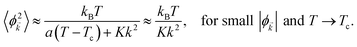 | (B5) |
Transforming back to real space, we have
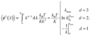 | (B6) |
Hence 〈ϕ2()〉 is finite in 3D but diverges in 1D and 2D. That is, long wavelength fluctuations would destroy sharp phase transitions in 1D and 2D, but in 3D the fluctuations are just perturbations.
 . Now consider the consequence of displacing every second atom by a small amount δ as shown by the red dots in Fig. 22. After such a distortion, the periodicity of the 1D crystal becomes 2a instead of a, and the reciprocal lattice vector changes from a*old = 2π/a to a*new = π/a, with a gap at the boundary of the first Brillouin zone, π/2a, which coincides with the Fermi wavevector kF. What Peierls has shown is that such a distortion is always favored because it lowers the overall energy of the system; hence at T = 0 a one dimensional conductor will inevitably becomes a semiconductor. The strength of Peierls' argument is that the conclusion is always true in the limit of δ → 0. Below we show heuristically the outline of Peierls' argument.
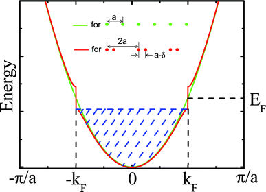 | ||
| Fig. 22 Peierls distortion in a one dimensional metallic crystal. The green (red) line corresponds to the crystal lattice and energy dispersion relation without distortion (with distortion). | ||
After the Peierls distortions, the electronic dispersion is shown by the red line in Fig. 22. As the electrons fill the lower band, the electronic energy is clearly lowered. To show how much the energy is lowered, consider the energies of the kF, −kF states, which are now Bragg-coupled:

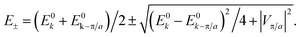 | (B7) |
The amount of total electronic energy lowering is given by
 | (B8) |
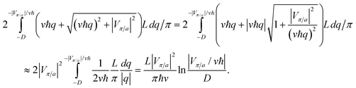 | (B9) |
For a small |Vπ/a|, the magnitude of this term always dominates over any term that is on the order of |Vπ/a|2, since it is logarithmic in character. But the elastic energy increase of the lattice distortion must be proportional to |Vπ/a|2 because the elastic energy is always quadratic in the strain, in either the real space or the k space. Therefore, the lowering in the electronic energy always dominates over the increase of lattice distortion energy in the limit of |Vπ/a| → 0, and the Peierls distortion is favored in a 1D conductor.
It should be noted that the Peierls distortion relies on electron–phonon coupling, just as in the case of superconductivity. Therefore in 1D it is not at all clear that a metallic system can become superconducting when the Peierls distortion is also possible. From our experimental results, it seems that the Peierls distortion can be suppressed, relative to the superconductivity, through either dielectric screening or lateral Josephson coupling.
Appendix C
Ginzburg–Landau theory and the Langer–Ambegaokar–McCumber–Halperin theory for 1D superconductors
![[r with combining right harpoon above (vector)]](https://www.rsc.org/images/entities/b_i_char_0072_20d1.gif) ) = |ψ()|eiφ(), with |ψ()|2 = ns() denoting the local density of superconducting electrons. The value of the order parameter (also called the wave-function) depends on the temperature, magnetic field and the spatial position. Basic to the GL theory is that the free energy F can be expanded in the following series form46
) = |ψ()|eiφ(), with |ψ()|2 = ns() denoting the local density of superconducting electrons. The value of the order parameter (also called the wave-function) depends on the temperature, magnetic field and the spatial position. Basic to the GL theory is that the free energy F can be expanded in the following series form46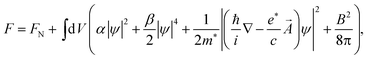 | (C1) |
![[A with combining right harpoon above (vector)]](https://www.rsc.org/images/entities/b_i_char_0041_20d1.gif) denotes the vector potential,
denotes the vector potential, ![[B with combining right harpoon above (vector)]](https://www.rsc.org/images/entities/b_i_char_0042_20d1.gif) = ∇ × denotes the magnetic field, ℏ is the Planck's constant, and α, β are the phenomenological parameters. Minimizing the free energy variationally with respect to ψ and leads directly to the GL differential equations
= ∇ × denotes the magnetic field, ℏ is the Planck's constant, and α, β are the phenomenological parameters. Minimizing the free energy variationally with respect to ψ and leads directly to the GL differential equations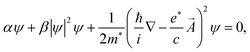 | (C2) |
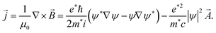 | (C3) |
By substituting ψ() = |ψ()|eiφ() into eqn (C3), we obtain
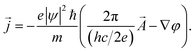 | (C4) |
Together with the Maxwell equations we get
 | (C5) |
 | (C6) |
 is the decay length, denoted as the magnetic (London) penetration length. Since inside a homogeneous superconductor the solution must be a constant, and the only solution to eqn (C6) with a constant B is B = 0; one is thereby led to the Meissner effect.
Besides the magnetic penetration length λ, another characteristic length for a superconductor is the coherence length ξ that characterizes the scale of spatial variations for the order parameter. It is given by  , where ξ0 is the zero temperature coherence length and Tc is the transition temperature. The ratio κ = λ/ξ is called the Ginzburg–Landau parameter, whose value for type I superconductors lies in the range
  , and
, and  for type II superconductors.
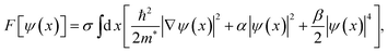 | (C7) |
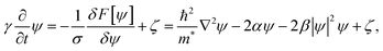 | (C8) |
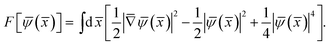 | (C9) |
The over-bar denotes the dimensionless quantities, obtained with F scaled by σξα20(Tc − T)2/β = ε0, which is the superconducting condensation energy for a volume σξ; ψ is scaled by  and x by the correlation length ξ(T). The corresponding dimensionless equation of motion is
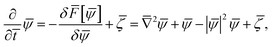 | (C10) |
Consider the current carrying meta-stable states in a closed superconducting ring. The periodic boundary condition for ψ is imposed by ψ(−l/2) = ψ(l/2), where l is the circumference of the ring. Meta-stable current carrying states ψn are obtained as the solutions to the stationary Ginzburg–Landau equation
 | (C11) |
 | (C12) |
 represents a meta-stable current-carrying superconducting state. To depict such a state, we note that since the magnitude of the wave function is rather rigid at a fixed temperature below Tc (owing to the fact that its variation involves much larger energy than the phase variation), a picture of this meta-stable state, shown in Fig. 23,62 involves only the phase variation as a function of x. The current density in the state is given by
 | (C13) |
 , with
  being the critical upper bound for kn beyond which there is no more solution to eqn (C11). The larger the winding number n the larger the carrying current, and the higher would be the free energy of the meta-stable state. Fig. 24 shows the scaled free energy F evaluated along the minimal energy path connecting a sequence of the meta-stable (−8, −7, …, −1, 1, …, 7, 8) and stable states (n = 0), plotted as a function of the arc length s in the ψ(x) functional space.62 This figure is numerically evaluated by using the string method.62 It should be noted that there is a potential barrier between neighboring meta-stable states, and this potential barrier becomes smaller for the higher current-carrying states.
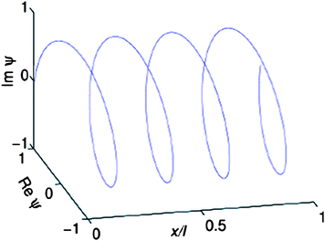 | ||
| Fig. 23 The order parameter ψ for a 1D superconductor with a winding number of 4. Adapted from ref. 62. | ||
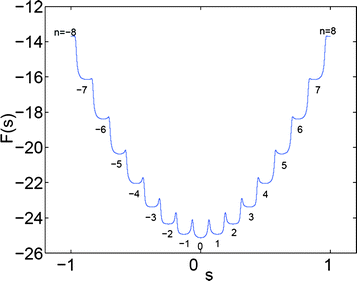 | ||
| Fig. 24 Free energy F evaluated along the minimal energy path connecting a sequence of meta-stable (−8, −7, …, −1, 1, …, 7, 8) and the stable state (n = 0). Here s represents the arc length along the minimal energy path in the functional space of ψ(x). Each metastable minimum represents a winding number configuration. Hence n = 4 has the configuration shown in Fig. 23. Adapted from ref. 62. | ||
As long as the wavefunction remains in a meta-stable state, the carrying current does not generate any voltage. That is, the system is still superconducting. However, in the presence of thermal fluctuations, one meta-stable state can transit to another by crossing a potential barrier. That is, in a thermal bath the lifetime of these meta-stable states is finite. Now consider a 1D superconducting wire being connected to a current source. Whenever a meta-stable state n transits to the lower free energy meta-stable state n − 1, the carrying current of the system will decrease as well. Since the current source has to maintain the current at a fixed value, it will push the system back up to the meta-stable state n again. In this process work is done by the external source, i.e., dissipation has occurred. Another way of saying the same thing is that a voltage will appear as a consequence of the thermally induced transitions between the meta-stable, current-carrying states. The magnitude of the voltage is directly proportional to the rate of such transitions through the following relation
| 2πΓps = 2 eV/ℏ, with Γps = Ωexp [−ε0ΔF/kBT], | (C14) |
From the above basic concept of the Langer–Ambegaokar–McCumber–Halperin theory42–44 we can understand how a 1D superconductor acquires finite resistance. Since the height of the potential barriers separating the meta-stable states is directly proportional to the cross sectional area (since the energy unit ε0 is linearly proportional to σ), with increasing cross sectional area as the system approaches 3D, the transition rate exponentially decreases and thereby the resistance disappears.
Acknowledgements
We thank Z. K. Tang, N. Wang, C. T. Chan and X. X. Zhang for their long term collaboration. We also acknowledge C. Ieong, J. T. Ye, Q. C. Zhang, F. Y. Jiang, B. Zhang, O. Tang, T. Zhang, Y. Zheng and H. Xie for their contributions to this project over the past few years. This work has been supported by the Research Grants Council of Hong Kong, Grants HKUST9/CRF/08, CA04/04.SC02, DSC104/05.SC01, VPAAO04/05.SC01 and SEG_HKUST03.References
- A. Oberlin and M. Endo, J. Cryst. Growth, 1976, 32, 335–349 CrossRef CAS.
- S. Iijima, Nature, 1991, 354, 56–58 CrossRef CAS.
- M. S. Dresselhaus, G. Dresselhaus and R. Saito, Phys. Rev. B: Condens. Matter Mater. Phys., 1992, 45, 6234–6242 CrossRef CAS.
- N. Hamada, S. Sawada and A. Oshiyama, Phys. Rev. Lett., 1992, 68, 1579–1581 CrossRef CAS.
- R. Saito, M. Fujita, G. Dresselhaus and M. S. Dresselhaus, Phys. Rev. B: Condens. Matter Mater. Phys., 1992, 46, 1804–1811 CrossRef CAS.
- R. H. Baughman, A. A. Zakhidov and W. A. de Heer, Science, 2002, 297, 787–792 CrossRef CAS.
- S. J. Tans, A. R. M. Verschueren and C. Dekker, Nature, 1998, 393, 49–52 CrossRef CAS.
- J. Kong, N. R. Franklin, C. W. Zhou, M. G. Chapline, S. Peng, K. J. Cho and H. J. Dai, Science, 2000, 287, 622–625 CrossRef CAS.
- W. A. Deheer, A. Chatelain and D. Ugarte, Science, 1995, 270, 1179–1180 CAS.
- S. S. Fan, M. G. Chapline, N. R. Franklin, T. W. Tombler, A. M. Cassell and H. J. Dai, Science, 1999, 283, 512–514 CrossRef CAS.
- N. D. Mermin and H. Wagner, Phys. Rev. Lett., 1966, 17, 1133–1136 CrossRef CAS.
- P. C. Hohenberg, Phys. Rev., 1967, 158, 383–386 CrossRef CAS.
- R. E. Peierls, Quantum Theory of Solids, Clarendon Press, Oxford, 1995 Search PubMed.
- L. X. Benedict, V. H. Crespi, S. G. Louie and M. L. Cohen, Phys. Rev. B: Condens. Matter Mater. Phys., 1995, 52, 14935–14940 CrossRef CAS.
- Z. K. Tang, L. Y. Zhang, N. Wang, X. X. Zhang, G. H. Wen, G. D. Li, J. N. Wang, C. T. Chan and P. Sheng, Science, 2001, 292, 2462–2465 CrossRef CAS.
- A. Kasumov, M. Kociak, M. Ferrier, R. Deblock, S. Gueron, B. Reulet, I. Khodos, O. Stephan and H. Bouchiat, Phys. Rev. B: Condens. Matter Mater. Phys., 2003, 68, 214521 CrossRef.
- M. Kociak, A. Y. Kasumov, S. Gueron, B. Reulet, I. I. Khodos, Y. B. Gorbatov, V. T. Volkov, L. Vaccarini and H. Bouchiat, Phys. Rev. Lett., 2001, 86, 2416–2419 CrossRef CAS.
- I. Takesue, J. Haruyama, N. Kobayashi, S. Chiashi, S. Maruyama, T. Sugai and H. Shinohara, Phys. Rev. Lett., 2006, 96, 057001 CrossRef CAS.
- R. Lortz, Q. C. Zhang, W. Shi, J. T. Ye, C. Y. Qiu, Z. Wang, H. T. He, T. Z. Qian, Z. K. Tang, N. Wang, X. X. Zhang, J. N. Wang, C. T. Chan and P. Sheng, Proc. Natl. Acad. Sci. U. S. A., 2009, 106, 7299–7303 CrossRef CAS.
- Z. Wang, W. Shi, H. Xie, T. Zhang, N. Wang, Z. K. Tang, X. X. Zhang, R. Lortz, P. Sheng, I. Sheikin and A. Demuer, Phys. Rev. B: Condens. Matter Mater. Phys., 2010, 81, 174530 CrossRef.
- C. Ieong, Z. Wang, W. Shi, Y. X. Wang, N. Wang, Z. K. Tang, P. Sheng and R. Lortz, Phys. Rev. B: Condens. Matter Mater. Phys., 2011, 83, 184521 CrossRef.
- H. D. Sun, Z. K. Tang, J. Chen and G. Li, Solid State Commun., 1999, 109, 365–369 CrossRef CAS.
- N. Wang, Z. K. Tang, G. D. Li and J. S. Chen, Nature, 2000, 408, 50–51 CrossRef CAS.
- S. Qiu, W. Pang, H. Kessler and J. L. Guth, Zeolites, 1989, 9, 440–444 CrossRef CAS.
- P. Launois, R. Moret, D. Le Bolloc'h, P. A. Albouy, Z. K. Tang, G. Li and J. Chen, Solid State Commun., 2000, 116, 99–103 CrossRef CAS.
- M. S. Dresselhaus, G. Dresselhaus, R. Saito and A. Jorio, Phys. Rep., 2005, 409, 47–99 CrossRef.
- J. T. Ye and Z. K. Tang, Phys. Rev. B: Condens. Matter Mater. Phys., 2005, 72, 045414 CrossRef.
- I. L. Li, G. D. Li, H. J. Liu, C. T. Chan and Z. K. Tang, Appl. Phys. Lett., 2003, 82, 1467–1469 CrossRef CAS.
- H. J. Liu and C. T. Chan, Phys. Rev. B: Condens. Matter Mater. Phys., 2002, 66, 115416 CrossRef.
- K. P. Bohnen, R. Heid, H. J. Liu and C. T. Chan, Phys. Rev. Lett., 2004, 93, 245501 CrossRef.
- K. P. Bohnen, R. Heid and C. T. Chan, J. Phys.: Condens. Matter, 2009, 21, 084206 CrossRef.
- D. Connetable, G. M. Rignanese, J. C. Charlier and X. Blase, Phys. Rev. Lett., 2005, 94, 015503 CrossRef CAS.
- R. Barnett, E. Demler and E. Kaxiras, Phys. Rev. B: Condens. Matter Mater. Phys., 2005, 71, 035429 CrossRef.
- K. Kamide, T. Kimura, M. Nishida and S. Kurihara, Phys. Rev. B: Condens. Matter Mater. Phys., 2003, 68, 024506 CrossRef.
- D. Carpentier and E. Orignac, Phys. Rev. B: Condens. Matter Mater. Phys., 2006, 74, 085409 CrossRef.
- J. Gonzalez and E. Perfetto, Phys. Rev. B: Condens. Matter Mater. Phys., 2005, 72, 205406 CrossRef.
- M. Ferrier, F. Ladieu, M. Ocio, B. Sacepe, T. Vaugien, V. Pichot, P. Launois and H. Bouchiat, Phys. Rev. B: Condens. Matter Mater. Phys., 2006, 73, 094520 CrossRef.
- N. Murata, J. Haruyama, Y. Ueda, M. Matsudaira, H. Karino, Y. Yagi, E. Einarsson, S. Chiashi, S. Maruyama, T. Sugai, N. Kishi and H. Shinohara, Phys. Rev. B: Condens. Matter Mater. Phys., 2007, 76, 245424 CrossRef.
- Z. M. Li, J. P. Zhai, H. J. Liu, I. L. Li, C. T. Chan, P. Sheng and Z. K. Tang, Appl. Phys. Lett., 2004, 85, 1253–1255 CrossRef CAS.
- J. Zhai, Z. Li, H. Liu, I. Li, P. Sheng, X. Hu and Z. Tang, Carbon, 2006, 44, 1151–1157 CrossRef CAS.
- F. Jiang, J. Zhai, J. Ye, J. Han and Z. Tang, J. Cryst. Growth, 2005, 283, 108–114 CrossRef CAS.
- Z. Wang, Superconductivity in 4-Angstrom Carbon Nanotube Arrays, PhD thesis, The Hong Kong University of Science and Technology, 2011 Search PubMed.
- W. A. Little, Phys. Rev., 1967, 156, 396–403 CrossRef CAS.
- J. S. Langer and V. Ambegaokar, Phys. Rev., 1967, 164, 498–510 CrossRef.
- D. E. McCumber and B. I. Halperin, Phys. Rev. B: Condens. Matter Mater. Phys., 1970, 1, 1054–1059 CrossRef.
- T. Zhang, M. Y. Sun, Z. Wang, W. Shi and P. Sheng, Phys. Rev. B: Condens. Matter Mater. Phys., submitted. Search PubMed.
- M. Tinkham, Introduction to Superconductivity, McGraw-Hill, NY, 1975 Search PubMed.
- S. Doniach and B. A. Huberman, Phys. Rev. Lett., 1979, 42, 1169–1172 CrossRef CAS.
- B. I. Halperin and D. R. Nelson, J. Low Temp. Phys., 1979, 36, 599–616 CrossRef CAS.
- A. F. Hebard and A. T. Fiory, Phys. Rev. Lett., 1983, 50, 1603–1606 CrossRef CAS.
- H. Q. Ding and M. S. Makivic, Phys. Rev. B: Condens. Matter Mater. Phys., 1990, 42, 6827–6830 CrossRef.
- D. W. Abraham, C. J. Lobb, M. Tinkham and T. M. Klapwijk, Phys. Rev. B: Condens. Matter Mater. Phys., 1982, 26, 5268–5271 CrossRef CAS.
- P. Fulde and R. A. Ferrell, Phys. Rev., 1964, 135, A550–A563 CrossRef.
- A. I. Larkin and Y. N. Ovchinnikov, Sov. Phys. JETP, 1965, 20, 762–768 Search PubMed.
- R. Lortz, Y. Wang, A. Demuer, P. H. M. Bottger, B. Bergk, G. Zwicknagl, Y. Nakazawa and J. Wosnitza, Phys. Rev. Lett., 2007, 99, 187002 CrossRef CAS.
- B. Bergk, A. Demuer, I. Sheikin, Y. Wang, J. Wosnitza, Y. Nakazawa and R. Lortz, Phys. Rev. B: Condens. Matter Mater. Phys., 2011, 83, 064506 CrossRef.
- P. F. Seidel and S. G. Sullivan, Phys. Rev., 1968, 173, 679–682 CrossRef.
- H. J. Liu, Z. M. Li, Q. Liang, Z. K. Tang and C. T. Chan, Appl. Phys. Lett., 2004, 84, 2649–2651 CrossRef CAS.
- J. Gonzalez, Phys. Rev. B: Condens. Matter Mater. Phys., 2005, 72, 073403 CrossRef.
- E. Perfetto and J. Gonzalez, J. Phys.: Condens. Matter, 2006, 18, S2105–S2114 CrossRef CAS.
- V. L. Ginzburg and L. D. Landau, J. Exp. Theor. Phys., 1950, 20, 1064 CAS.
- T. Qian, W. Q. Ren and P. Sheng, Phys. Rev. B: Condens. Matter Mater. Phys., 2005, 72, 014512 CrossRef.
| This journal is © The Royal Society of Chemistry 2012 |