Microfluidic sorting of arbitrary cells with dynamic optical tweezers

Abstract

Optical gradient forces generated by fast steerable optical tweezers are highly effective for sorting small populations of cells in a lab-on-a-chip environment. The presented system can sort a broad range of different biological specimens by an automated optimisation of the tweezer path and velocity profile. The optimal grab positions for subsequent trap and cell displacements are estimated from the intensity of the bright field image, which is derived theoretically and proven experimentally. We exhibit rapid displacements of 2 μm small mitochondria, yeast cells, rod-shaped bacteria and 30 μm large protoplasts. Reliable sorting of yeast cells in a microfluidic chamber by both morphological criteria and by fluorescence emission is demonstrated.

---

Introduction

For many years, fluorescence-activated cell sorting (FACS) has been the standard technique for sorting biological cells in suspension, featuring high throughput, purity, and yield.¹ Besides the problem that available FACS machines are expensive and demanding to operate, the large numbers of cells needed for calibration and a sometimes lethal stress induced to the cells by shear forces limit the field of applications.

Lab-on-a-chip systems promise to overcome this drawback.² Existing microfluidic cell sorters operate either via redirecting flow (electro-osmosis³ or valves^4,5,6), or via magnetic,⁷ dielectrophoretic,^8,9,10,11 or optical forces acting directly on cells or on a droplet encapsulating them.

Laser optical actuation is especially advantageous, since properly chosen forces are strong enough, but usually non-damaging. Furthermore, spatial light distributions can be switched rapidly in intensity and shape, such that the microfluidic chip does not need any electrodes or active layers – in contrast to systems based on dielectrophoresis. Avoidance of cell encapsulation facilitates further investigation and recultivation.

All cell sorters exploiting optical forces which have been presented so far are designed for cells with a specific shape and size.¹² Passive optical cell sorters use a specifically designed static light distribution, typically an optical lattice with a designed grating width to deflect cells in a microfluidic channel.^13,14,15 Passive sorters can only sort by differences in refractive index, in size or in shape. In contrast, active optical sorters are able to sort nearly identical cells according to small differences in features, which are typically encoded by a spatial fluorescence distribution. Existing active optical sorters work with moderately focused beams, which are intensity modulated but not displaced.^16,17,18,19 In both the passive and active sorting modes, force fields are distributed over a larger area and depend on the size and refractive index of the suspended objects. Hence, objects varying in these two parameters cannot be sorted without re-designing the system. In contrast, an optical point trap from a highly focused laser beam, also known as optical tweezers, produces significantly higher optical forces when the same laser power is applied to the cell.

In this paper, we present an optical particle sorter that uses rapid steerable optical traps to displace cells within a laminar flow inside a microchannel. Cells not grabbed by the optical tweezers stream into a different reservoir than those actively displaced to a parallel streamline. The system is preferably suitable for small populations of a few hundred or thousand cells or for sorting out rare events. A similar system has been realized only recently for a specific type of cell.²⁰ However, our sorter can handle arbitrary cells since neither channel structure nor the forces of the optical tweezers need to be changed for a specific kind of cell. The optimal grab position for each specific cell can be determined by the intensity of bright field CCD images. In this paper, we derive and explain the relation between the bright field intensity and the expected optical force. Based on this information, an optimized optical trap path can be generated ensuring a rapid and secure displacement of each cell within the channel. Before activation of the optical trap, each cell can be classified by a bright field or a fluorescence image with 300 nm optical resolution, allowing sorting also by morphological criteria and expression of fluorescent markers. Moreover, an optically transparent microfluidic chamber suitable for mass production is used. The system is designed as an add-on for a standard inverted microscope and thus can be run in any standard lab.

The sorter's capabilities are demonstrated in the first place by displacements of mitochondria, bacteria, yeast, and plant protoplasts at various displacement speeds or frequencies. In addition, a population of yeast cells is sorted inside a microchannel, where cells are classified by both their size and their fluorescence intensity in the same run.

Experimental

Optical system

The setup of the sorter (Fig. 1) uses an inverted microscope (Zeiss, Axiovert 200) as a platform. The objective lens (Zeiss, C-Apochromat, 40×, NA 1.2) is a coverslip-corrected water immersion lens and is used for imaging and focusing of the trapping laser, which operates in the near-infrared at 1064 nm (Alphalas Lasers, Monopower-1064-10W-SM). Images are captured with a CCD camera (Prosilica, GC1350H) with a full frame rate of 12.9 fps. An additional telescope system (0.5×) in front of the camera leads to an overall magnification of 20×. Fluorescence is excited with a mercury lamp (Zeiss, HXP120) during the integration time of the CCD; bright field images are illuminated software-triggered by a LED (Lumileds, Luxeon I). Both channels can be overlaid in the software's camera window. The focused laser forming the optical trap is steered in its position in two dimensions by galvanometric mirrors (GSI, VM500+) deflecting the collimated laser in a plane conjugate to the pupil plane of the objective lens. After having received their signals by a D/A card (National Instruments, PCIe-6259), the mirrors can deflect at a 200 μs response and at 1 μs temporal resolution. The optical power in the focal plane was 270 mW for experiments with different cells on the piezo stage and 67 mW for sorting of yeast cells in the microchannel.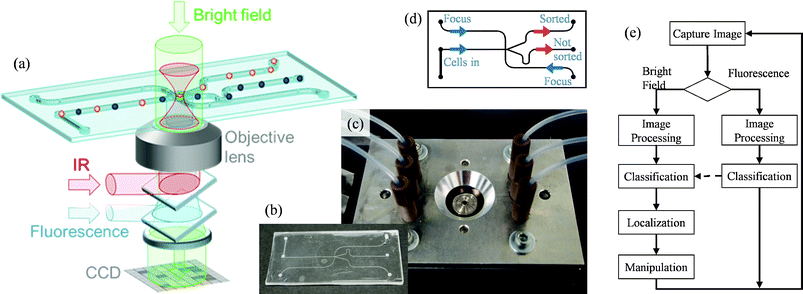

Fig. 1 (a) Cells within the microchannel can be localized and classified with bright field (green) and/or fluorescence (blue) illumination through a high NA objective. Once a cell is classified, it is moved by optical tweezers (red) to a streamline of laminar flow which leads to the outlet for sorted cells. (b,c) Photographs of microfluidic chamber inserted into its chip holder and connected to tubing. (d) Fluid flow diagram with 3 inlets (blue) and 2 outlets (red). (e) Logical flow diagram for a popular sorting mode: 1. classification by the intensity in the fluorescence channel; 2. Additional classification by the size in the bright field channel. After positive classification, the bright field image is used to determine the location for the most efficient manipulation.

This arrangement is sketched in Fig. 1. It enables classification of cells (i) by the feature information delivered by bright field images, such as size, shape or more complex morphology, (ii) by the intensity of fluorescence light, or (iii) both. A logical flow diagram for this last option is shown in Fig. 1e. Only if a cell is classified positive in a fluorescence image (feature ii) and in the subsequent bright field image (feature i) is it localized precisely and moved by the optical trap to a streamline directed towards the channel for sorted cells.

Microfluidic system

The microfluidic sorting chip can be produced with technologies suitable for rapid prototyping and mass production.²¹ For the experiments presented here a prototype was used. Channels of 100 μm in width and 80 μm in height were precision milled in 1.5 mm thick Cyclic Olefin Copolymer (COC) 5013 (Fig. 1a). Inlets and outlets were drilled with a diameter of 0.5 mm. The chip was covered with a 140 μm thick foil of COC 8007, serving as the bottom of the channel. For sealing, both parts were cleaned with isopropanol and deionized water, exposed to cyclohexane vapour for 130 s, and subsequently pressed against each other with a hard rubber roll. The prototype was put into an aluminium frame and connected to a multichannel syringe pump (Cetoni, neMESYS) and output reservoirs (Eppendorf tube) via fittings and tubing (Upchurch Scientific, PEEK, 1/16′′ OD, 170 μm ID) (Fig. 1b,c).

Cell preparation

Mitochondria from fresh murine liver tissue was prepared as described earlier.²² Mitochondria are roundish cell organelles of about 2 μm diameter, have a membrane and are called cells throughout the rest of this paper. Bacillus subtilis are rod-shaped bacteria with a diameter of about 1 μm and a length of about 4 μm (for preparation see ref. 23).

Protoplasts from the root of Arabidopsis thaliana with a diameter of 40 μm were chosen for the experiments (for preparation see ref. 24).

Yeast cells (Saccharomyces cerevisiae) were stained with MitoTracker Green (Invitrogen) as described in the manual, but with a five times higher concentration of stock solution. Stained and unstained suspensions were mixed in a 1 : 1 ratio, yielding a concentration of 4 × 10⁷ cells per microliter.

Viability tests with Trypan Blue (Sigma Aldrich) were performed on a population immediately extracted after sorting and on an unsorted control group by counting under the microscope.

Determination of the optimal trap path

Optical trapping forces are mainly dominated by the optical gradient force (dipole force), whereas the disadvantageous scattering force (radiation pressure) is to be minimized.²⁵ At laser powers of about 100 mW, optical tweezers operated at λ = 1.06 μm can exert optical forces of 10–300 pN, depending on the polarisability α of the particle or of a part of the cell. A cell can then be moved through the medium by the trap as long as the optical gradient force is at least as high as the viscous drag force, F_grad ≥ F_γ, which depends on its size and the drag speed. For an efficient displacement of a cell to another fluid stream line, it is essential to grab the cell at a suitable position and displace it as fast as possible in a minimal period of time.

In order to find an efficient grab location with maximal gradient force, information extracted from bright field images can be used.

The optical gradient force F_grad on a volume V of dipoles at position b can be described²⁶ with

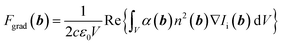where c is the speed of light and ε₀ the vacuum permittivity. The polarisability α, the refractive index n and the incident intensity of the trapping light I_i all vary with b. If we neglect absorption (α and n real) and approximate the extent of the trapping focus or the trapped particle to be small, the integral in eqn (1) 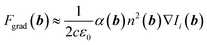can be omitted, such that eqn (2) is valid.

With the Clausius-Mossotti relationship, the polarisability can be written as α(b) = (n²(b) − (n(b) + Δn(b))²)/(n²(b) + 2(n(b) + Δn(b))²), where Δn is the difference of the refractive index to a neighboring position b + Δb. After a 1st order Taylor approximation of α around Δn = 0, we find α ≈ 2Δn/(3n) such that the optical gradient force can be written as

which means that F_grad is approximately proportional to the local change of the refractive index Δn at position b.

The spatial variation Δn can be extracted from bright field images. For spatially coherent illumination (Koehler aperture closed), we get an interference pattern directly behind the focal plane described by:

where [Fraktur I]is the bright field intensity, [Fraktur I]_i the incident intensity, [Fraktur I]_s the scattered intensity, and ΔΦ the phase shift between the two waves inside the volume element V. It is a complex task to determine the intensity within a thick, scattering cell. But for positions close to the cell membrane, where Δn are maximal, it can be assumed that the light's incidence angle and the emergent angle of the reflected light are both perpendicular to the cell's normal in the focal plane, such that θ_i ≈ θ_r ≈ 90° and therewith ΔΦ ≈ π and cos(ΔΦ(θ)) ≈ −1. Inserting [Fraktur I]_s = [Fraktur I]_ir_A², into eqn (4) where r_A(ΔΦ) is the reflection coefficient, we find:

[Fraktur I](b) = [Fraktur I]_i(b)(1 − r_A)² (5)

Again, for large angles, the reflection coefficient can be simplified to r_A ≈ Δn/(Δn + 2n). After a 1st order Taylor approximation of (1 − r_A)² around Δn = 0, we find [Fraktur I](b)/[Fraktur I]_i(b) ≈ 1 − Δn(b)/n(b).

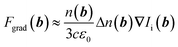
In total, there is a direct relationship between the intensity change Δ[Fraktur I] = [Fraktur I]_i(b) − [Fraktur I](b) in the bright field image on the CCD, the gradient of refractive index Δn(b), and optical gradient force F_grad(b) according to eqn (3):

Δ[Fraktur I](b) ∝ Δn(b) ∝ F_grad(b) (6)

Fig. 2 illustrates the implications, which can be made for all four cell types. If a cell shall be moved along the yellow-dashed line, the magnitude of the optical forces can be expected to be highest where Δ[Fraktur I] has a minimum. This is exactly the location where the sorter can grab a cell, independently of its actual size or shape.

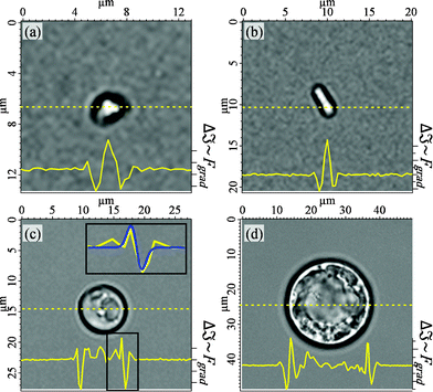Fig. 2 Determination of the optimal trapping positions on four different cell types ((a) mitochondrion, (b) bacterium, (c) yeast cell, (d) protoplast) with transmission intensity of bright field illumination. A local minimum in the image intensity Δ[Fraktur I] indicates a high refractive index gradient Δn and thus results in high trapping forces F_grad. The inset of (c) illustrates the approximation of the force profile according to eqn (6).

Fig. 3a illustrates how the relation in eqn (6) can be used to determine the 2D coordinates of a trap path for sorting in the x-direction. First, the minimum of Δ[Fraktur I] in the x-direction (search starts at cell centre) is localized. This point, where highest trapping forces are expected, is defined as x_cell. If cells have different sizes or if they enter the channel slightly out of focus, the precision of finding x_cell can vary and so there is a risk of missing some cells. In order to trap every cell with a high reliability, it is beneficial to sacrifice a bit of displacement time and place the trap initially at a small distance x_i closer to the cell centre (x_i = 15% of distance between x_cell and cell centre). Starting from this initial position x₀ (see Fig. 3a), the trap moves with a velocity v_trap(t = 0) = v_min in the x-direction. It accelerates constantly over a distance x_a, until it reaches its maximum velocity v_max. On the remaining and major part of the trap path, the trap moves with v_max. The idea behind this velocity profile is that trap and cell can find their optimal position relative to each other (x_trap(t > τ_a) = x_cell(t > τ_a)). The farther the trap has moved from x₀ towards x_cell, the more likely it is that the trapping force F_grad has reached its maximum and exceeds the viscous drag force F_γ = 6πRζv_cell (R = cell radius, ζ = viscosity of fluid medium). In the y-direction, the trap moves constantly with the velocity of the fluid to avoid additional viscous drag forces. Since all cells flow in the same height directly above the bottom of the fluid chamber, the optimal z-position between chamber, cells and trap can be achieved by simply focusing the cells in the focal plane, which is the trap's z-position.

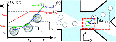Fig. 3 (a) Trajectories x_trap(t) of the trap and x_cell(t) of the cell enabling efficient displacements. The optical trap is initially positioned close to the cell membrane within the cell body. Starting at x₀ with velocity v_min, the cell is accelerated over a short distance x_a. During this time τ_a, the trap finds the most polarizable part of the cell. Most of the displacement is performed with a maximal trap velocity of v_max. (b) Sketch of the chamber and the sorting geometry. The cell suspension is hydrodynamically focused and directed to the lower output by default. Image processing is performed within the outer red-dashed rectangle. Cells detected and classified within the inner rectangular region are dragged over a distance Δx_cell to a streamline ending in the upper outlet.

When a cell is released after the velocity dependent displacement time τ(v_max) = (2x_a)/(v_max − v_min) + (d − x_a)/v_max, its centre has moved in total a distance x_cell(τ) = Δx_cell in sorting direction (Fig. 3b). To allow undisturbed displacement and regular transport of cells, the suspension is enclosed by sheath flows containing buffer medium. Image processing consumes computing power and thus is restricted to an area marked with the larger red-dashed rectangle. Once a cell is classified as positive within the small red rectangle (sorting region), it is sorted according to the described trap path. Cell positions can be recorded immediately before and after dragging.

Software

The operating software is written in Python using SciPy/NumPy modules for calculations and image processing. Image analysis consists of the following steps: (1) subtraction of background, (2) thresholding, (3) binary dilation, (4) fill holes, (5) binary erosion, and (6) labelling of all remaining objects. Image processing takes about 15 ms per frame on a 3 GHz CPU (Intel, Core 2 Duo). Classification and localization of cell centres and trapping positions depend on the number of labelled particles and consume around 6 ms. Coordinates of the best trap path are usually calculated in less than 1 ms.

Results and discussion

Determination of displacement efficiency for different cell types

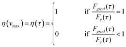
Although the sorter can handle a broad variety of cells in a flexible way, it is important to know how fast different types of cells can be moved (v_max) or how short displacement times τ can be. In order to address this question in an automated and reproducible way, the flow of the medium and the cells in the microchannel was generated by moving a piezo stage (MCL, Nano-View) back and forth with a random displacement in the orthogonal direction. As classification requirements, cells had only to be within a certain size range in the bright field image.

As an invariable sorting condition, a nominal displacement distance of d = 40 μm and an acceleration distance of x_a = 8 μm were chosen, comparable to the situation in the microchannel. Thereby, one can define a displacement efficiency η(τ) = Δx_cell(τ)/d, where Δx_cell is the actual displacement. One can expect

which means that the sorting efficiency should drop down rapidly as soon as F_γ exceeds F_grad. η can be increased with stronger optical forces F_grad and with smaller cell radii R.

As illustrated in the example of a yeast cell in Fig. 4a, cells were moved in flow direction (y-direction) by the piezo stage with a velocity of v_flow = 80 μm s⁻¹. Once they entered the sorting region, they were immediately displaced, released, and further transported in flow direction by the medium. For the next cycle, flow and sorting direction were flipped and the x-position of the cell was changed by a random value δx between −5 μm and +5 μm since the cell's x-position in the microchannel also varies within a similar range. The trap velocities v_min and v_max were increased after 10 cycles, such that after 200 cycles 20 different velocity pairs were applied. Immediately before and after sorting of each cycle, cell positions (centre-of-mass) were recorded, as well as the displacement distance Δx_cell and the displacement time τ. These records are plotted in Fig. 4b for the case of Bacillus subtilis. As the maximum trap speed v_max increases, τ decreases. At the beginning, the measured displacement distance in x-direction Δx is close to d, but with increasing speeds and rates 1/τ the displacement Δx drops off abruptly and significantly, since F_grad < 6πRηΔx/τ. We did not evaluate cycles, where a cell was dragged out of the trap due to too high trap velocities v in a previous cycle, i.e. when v × τ = Δx < 0.9 × 40 μm.

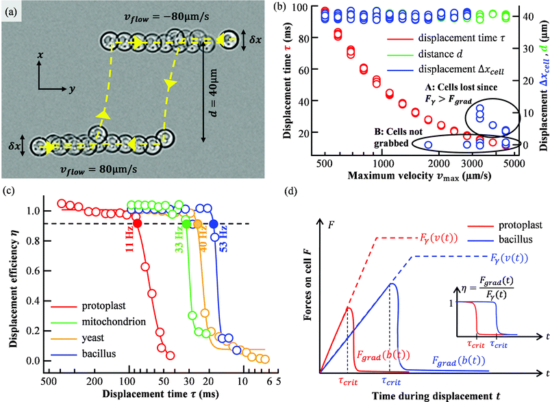Fig. 4 Displacement of different cells out of a flow. (a) Flow in a microchannel is emulated with a moving piezo stage at v_flow = 80 μm s⁻¹. Cells can be repeatedly and automatically displaced with the optical trap by reversion of the sorting direction after each “flow-through”. 2 cycles through the sorting region are marked with yellow dashed lines. δx indicates the flow position uncertainty along x, d is the nominal displacement. (b) The measured displacement duration τ (red), the nominal displacement distance d (green), and the actual displacement distance (blue) are recorded as a function of maximum trap speed v_max. (c) The displacement efficiency η as a function of displacement time η for all four cell types. Efficiency drops abruptly for a critical displacement time τ_crit. Possible sorting rates 1/τ_crit are given for η = 0.9. (solid markers). The solid lines represent sigmoidal fits to estimate the probabilities of correct sorting. (d) Qualitative change of optical force F_grad and viscous drag force F_γ over time for the case that a cell drops out of the trap during acceleration. At τ_crit the optical force can no longer counteract the viscous drag force and efficiency drops to zero.

It can be observed that there are two reasons for the efficiency to drop below η = 1. In cycles marked with A, the cell dropped out of the trap during acceleration exactly when the viscous drag force F_γ becomes higher than the optical trapping force F_grad. In cycles marked with B, however, cell and optical trap cannot find their optimal position relative to each other and thus the cell is not displaced at all. These errors can in principle be eliminated by giving the image processing algorithm more real-time properties, which improves the estimate of how far a cell will have moved along y until the optical trap becomes active. These sorting errors due to missing a cell's cross-section only occur for very small cells.

In Fig. 4c, the displacement efficiencies η(τ) = Δx_cell(τ)/d for protoplasts, mitochondria, yeast cells, and rod-shaped Bacillus subtilis are plotted. Sigmoidal fits illustrate the drop in sorting probabilities for critical displacement rates 1/τ_crit for each cell type. All efficiencies with the same parameters are averaged and marked as dots. At the lower end of displacement rates, we find the protoplast, which is largest in radius (2R ≈ 20–30 μm) and thus has the highest hydrodynamic resistance F_γ. On the other end, the rod-shaped bacillus orients vertically inside the axial extended trap and thus maximizes the overall polarisability α, while experiencing modest friction forces due to a cross-section of 1 μm × 4 μm. In addition, it has a cell wall with a higher refractive index and higher structural α than the mitochondrion, which is only enclosed by a membrane. (Videos can be found as ESI S1–S4.†)

Fig. 4d gives a qualitative explanation for the drop of efficiency (region A in Fig. 4b). The efficiency η(t) is time dependent since both the optical gradient force F_grad and the viscous drag force F_γ increase with displacement time t. F_grad changes qualitatively according to ∼d/db exp(−b²/σ²) with the particle displacement b(t), which itself increases with time. F_γ increases with the particle velocity v(t), which also increases with time. As soon as the maximum optical force is reached, the particle drops out of the trap and the ratio of both forces drops abruptly. It is worth noticing that sorting can also work with efficiency below 1.0, since the optical trap can grab the same cell several times if flow rates and cell concentration do not reach the upper performance limit.

Sorting of yeast cells by fluorescence emission and by size

Besides fast and flexible displacements of different types of cells without recalibration, the possibility of using specific and complex classification criteria such as fluorescence distributions inside cells is a key advantage of our sorter.

Therefore, a population of yeast cells was sorted in a microfluidic chamber according to the classification rule depicted in Fig. 1e: a cell is only classified positive if it emits a fluorescence signal above a certain threshold value and if the found value for its size in the bright field channel lies within a defined range. For example, a cell with stained mitochondria of proper size would be classified positive, but both a cell without fluorescence or fluorescent material without a surrounding cell would be classified negative. Screenshots of this sorting procedure are shown in Fig. 5. In Fig. 5a, cells enter from the left and get hydrodynamically focused on a stream line, where they will end up in the lower outlet channel by default. The black spot at the upper focusing channel is a small damage due to heavy usage of the chip and did not affect functionality of the system. Fluorescence excitation is restricted to a central region, in order to reduce background intensity. Cells flow through the sorting region with a velocity of v_flow = 76 μm s⁻¹. In case of a positive classification after image processing, cells are displaced by the optical trap (40 μm in average) and continue on a stream line ending in the upper outlet channel. Bright field images were acquired Δt = 85 ms after fluorescence images, resulting in a shift of several micrometres in flow direction when both images are overlaid. The insets at the right side show a bright field and fluorescent image of a cell recorded with a magnification of 20 giving an impression how subcellular features can be addressed for classification. Two example situations shall be highlighted. Therefore, the area marked with the yellow square is magnified. In Fig. 5b, incoming cells A and B were fluorescent, cell C not. The two remaining cells in the upper right corner have already been sorted. The second image in the filmstrip was acquired 0.34 s later (one frame skipped) and shows that A and B have been sorted, while C is leaving the sorting region towards the lower channel.

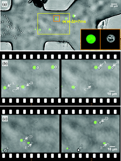Fig. 5 (a) Sorting of yeast cells in a microfluidic chamber by fluorescence level and size. Cells are classified by a fluorescence image (see green spots in the excitation region) and are localized in the subsequent bright field image. Positively classified cells are sorted to the upper outlet. Inlet images (16 μm × 16 μm) give an impression of resolvable features for classification. In the image sequence (b), fluorescent cells (A, B) are sorted out, non-fluorescent ones (C) not. In sequence (c), the fluorescent cell D is sorted, while structure E is a small fluorescent particle and consequently ignored. The time difference between the left and the right frame of the sequences (b) and (c) is 0.34 s. (Video available online as ESI S5.†)

In Fig. 5c, D and E were both fluorescent, but the particle E was of sub-critical size. It was consequently classified negatively in the bright field channel and was not sorted. A video file with annotations appearing on the computer screen during operation can be found in the ESI (S5).†

Conclusions

We have presented an active optical cell sorter based on fast steerable optical tweezers. By self-optimization of the acting optical gradient force versus the drag force, the system is able to sort a variety of cells having different shapes and sizes. No intermediate calibration is necessary. We have derived how the optimal trapping force within a cell can be found from the bright field image of the cell. Currently, the sorter's through-put is limited to about 1 Hz. However, because of the high speed and reliability of the cell displacement by the trap, short sorting time periods τ could be identified. The measured τ ≈ 20 ms for Bacillus subtilis, 25 ms for yeast cells, 30 ms for 2 μm small mitochondria and 90 ms for large plant protoplasts could in principle result in sorting rates of 10–50 Hz. In particular, we were limited by the camera and the image processing, which can be sped up further by reducing the area of interest to the sorting region or using a faster and better camera than the simple CCD used in our approach. The key challenge is to adjust the microfluidic system in a way that cells enter the sorting region in a dense chain, without sticking together.

Sorting of yeast cells in a microfluidic chamber resulted in a recovery rate of 95% at a throughput of 1.4 cells s⁻¹. The recovery rate is defined as the fraction of those positively classified cells which reach the channel for sorted cells. 89% of the cells found in this channel were confirmed to be positive after sorting (11% false positive). This purity was only slightly lower than in a previously reported work,²⁰ but still very satisfying, since classification criteria were more challenging and neither the microfluidics nor the laser power was optimised for this type of cell. The purity will be further increased if those cells that stick together are ignored. Cell clusters were not treated differently during image processing. By doing so, either the number of false positive or false negative cells will be minimized.

A significant advantage of the system is the low degree of stress induced to cells. Previous works have shown that the risk of photo-damage due to the trapping laser light is very low, e.g. yeast cells can bear 180 mW of laser power over 50 s.²⁷ In our case the sorting time is less than 100 ms and therefore the potential photo-toxicity can be clearly neglected. For yeast, damage resulting from the microfluidic system and fluorescence staining could be excluded through additional viability tests with Trypan Blue. Both sorted cells and an analogue control group did not show significantly decreased viability (98.8% vs. 98.5%).

Moreover, protoplasts are very fragile and cannot be sorted in a FACS machine because of too strong accelerations, but are well sortable with optical tweezers.

More complex classification algorithms could easily be added, which may not only check for the size of a cell, but for more sophisticated morphological properties, e.g. if the nucleus is fluorescing and the cell is elongated, indicating an on-going cell division.

These advantages make an optical tweezers-based cell sorter with self-optimised trap dynamics a top candidate for sorting of small cell populations encoded with the most manifold features and characteristics.

Acknowledgements

We thank Aude Parnet for preparing protoplasts, Felix Dempwolff for preparing bacteria, and René Pflugradt for preparing mitochondria. We further thank Matthias Koch for a thorough reading of the manuscript. This study was supported by the Excellence Initiative of the German Federal and State Governments (EXC 294).

References

1. H. M. Shapiro, Practical Flow Cytometry, John Wiley & Sons, Inc., Hoboken, NJ, USA, 2003.
2. A. Lenshof and T. Laurell, Chem. Soc. Rev., 2010, 39, 1203–17.
3. P. S. Dittrich and P. Schwille, Anal. Chem., 2003, 75, 5767–74.
4. A. Y. Fu, H.-P. Chou, C. Spence, F. H. Arnold and S. R. Quake, Anal. Chem., 2002, 74, 2451–7.
5. A. Wolff, I. R. Perch-Nielsen, U. D. Larsen, P. Friis, G. Goranovic, C. R. Poulsen, J. P. Kutter and P. Telleman, Lab Chip, 2003, 3, 22–7.
6. A. R. Abate, J. J. Agresti and D. A. Weitz, Appl. Phys. Lett., 2010, 96, 203509.
7. D. Robert, N. Pamme, H. Conjeaud, F. Gazeau, A. Iles and C. Wilhelm, Lab Chip, 2011, 11, 1902–10.
8. U. Kim, J. Qian, S. A. Kenrick, P. S. Daugherty and H. T. Soh, Anal. Chem., 2008, 80, 8656–61.
9. K. Ahn, C. Kerbage, T. P. Hunt, R. M. Westervelt, D. R. Link and D. A. Weitz, Appl. Phys. Lett., 2006, 88, 024104.
10. A. T. Ohta, in IEEE/LEOS International Conference on Optical MEMS and Their Applications Conference, 2005, IEEE, 2005, pp. 83–84.
11. S. Park, Y. Zhang, T.-H. Wang and S. Yang, Lab Chip, 2011, 11, 2893–2900.
12. A. Jonás and P. Zemánek, Electrophoresis, 2008, 29, 4813–51.
13. P. T. Korda, M. B. Taylor and D. G. Grier, Phys. Rev. Lett., 2002, 89, 128301.
14. M. P. MacDonald, G. C. Spalding and K. Dholakia, Nature, 2003, 426, 421–4.
15. G. Milne, D. Rhodes, M. MacDonald and K. Dholakia, Opt. Lett., 2007, 32, 1144–6.
16. T. N. Buican, M. J. Smyth, H. a Crissman, G. C. Salzman, C. C. Stewart and J. C. Martin, Appl. Opt., 1987, 26, 5311.
17. M. M. Wang, E. Tu, D. E. Raymond, J. M. Yang, H. Zhang, N. Hagen, B. Dees, E. M. Mercer, A. H. Forster, I. Kariv, P. J. Marchand and W. F. Butler, Nat. Biotechnol., 2005, 23, 83–7.
18. T. D. Perroud, J. N. Kaiser, J. C. Sy, T. W. Lane, C. S. Branda, A. K. Singh and K. D. Patel, Anal. Chem., 2008, 80, 6365–72.
19. C.-C. Lin, A. Chen and C.-H. Lin, Biomed. Microdevices, 2008, 10, 55–63.
20. X. Wang, S. Chen, M. Kong, Z. Wang, K. D. Costa, R. A. Li and D. Sun, Lab Chip, 2011, 11, 3656–3662.
21. J. Steigert, S. Haeberle, T. Brenner, C. Müller, C. P. Steinert, P. Koltay, N. Gottschlich, H. Reinecke, J. Rühe, R. Zengerle and J. Ducrée, J. Micromech. Microeng., 2007, 17, 333–341.
22. R. Pflugradt, U. Schmidt, B. Landenberger, T. Sänger and S. Lutz-Bonengel, Mitochondrion, 2011, 11, 308–14.
23. C. D. Webb, P. L. Graumann, J. A. Kahana, A. A. Teleman, P. A. Silver and R. Losick, Mol. Microbiol., 1998, 28, 883–92.
24. A. Dovzhenko, C. Dal Bosco, J. Meurer and H. U. Koop, Protoplasma, 2003, 222, 107–11.
25. A. Rohrbach and E. H. Stelzer, J. Opt. Soc. Am. A, 2001, 18, 839–53.
26. A. Rohrbach, Phys. Rev. Lett., 2005, 95, 168102.
27. J. A. Grimbergen, K. Visscher, D. S. G. de Mesquita and G. J. Brakenhoff, Yeast, 1993, 9, 723–32.

---

Footnote

† Electronic supplementary information (ESI) available. See DOI: 10.1039/c2lc21099a

---