Calcium isotope measurement by combined HR-MC-ICPMS and TIMS

Abstract

We report a novel approach for the chemical purification of Ca from silicate rocks by ion-exchange chromatography, and a highly-precise method for the isotopic analysis of Ca—including the smallest isotope ⁴⁶Ca (0.003%)—by high-resolution multiple collector inductively coupled plasma source mass spectrometry (HR-MC-ICPMS), in combination with thermal ionization mass spectrometry (TIMS). Using this approach, we measured the Ca isotope composition of a number of terrestrial rock standards and seawater. Based on these data, we show that the non-mass-dependent abundances of μ⁴³Ca, μ⁴⁶Ca, and μ⁴⁸Ca (normalized to ⁴²Ca/⁴⁴Ca) can be measured with an external reproducibility of 1.8, 45 and 12.5 ppm, respectively, when measured by HR-MC-ICPMS and μ⁴⁰Ca and μ⁴³Ca to 80 and 23 ppm, respectively, when measured by TIMS (μ notation is the per 10⁶ deviation from the reference material). Comparison with earlier studies demonstrate that it is possible to measure the mass-dependent Ca isotope composition of terrestrial materials using HR-MC-ICPMS with an external reproducibility comparable to that typically obtained with double spike TIMS techniques. The resolution of the mass-independent ⁴³Ca, ⁴⁶Ca and ⁴⁸Ca data obtained by HR-MC-ICPMS represents more than a 45-, 120-, and 18-fold improvement, respectively, relative to earlier measurements obtained by TIMS. This improvement allows for a better understanding of the mass fractionation laws responsible for the mass-dependent fractionation of Ca present in natural samples and synthetic standards. For example, the presence of an apparent excess of ∼60 ppm in the μ⁴⁸Ca composition of the SRM 915a suggests that equilibrium fractionation processes have generated the mass-dependent fractionation of this material. In contrast, the absence of residual anomalies in the mass-independent composition of seawater implies that biogenic and inorganic processes of carbonate formation fractionate Ca kinetically from seawater. Finally, we note that SRM 915b has a mass-dependent and mass-independent Ca isotope composition that is within the resolution of our method identical to that of bulk silicate Earth (BSE). This observation, together with the potential heterogeneity in the ⁴⁰Ca composition of the SRM 915a inferred from our measurements, suggests that the SRM 915b is a better reference material to study the Ca isotope composition of terrestrial and non-terrestrial materials.

---

1 Introduction

Calcium has five stable isotopes, ⁴⁰Ca, ⁴²Ca, ⁴³Ca, ⁴⁴Ca and ⁴⁶Ca and one with an extremely long half-life (⁴⁸Ca). The isotopic abundance of naturally occurring Ca is dominated by ⁴⁰Ca, which makes up about 96.9% of the total abundance. The remaining five isotopes have abundances of 2.1% (⁴⁴Ca), 0.65% (⁴²Ca), 0.19% (⁴⁸Ca), 0.14% (⁴³Ca) and 0.003% (⁴⁶Ca). This results in a range of isotopic abundance that varies from the largest (⁴⁰Ca) to the smallest (⁴⁶Ca) isotope by a factor of about 24,000.

The nucleosynthesis of Ca isotopes consists of various mechanisms representing different stellar environments. ⁴⁰Ca is a primary isotope and is a product of He and Ne burning. ⁴²Ca, ⁴³Ca, ⁴⁴Ca and ⁴⁶Ca are at least partially produced as secondary isotopes during the s-process from ⁴⁰Ca. The overabundance of ⁴⁴Ca is a result of decay of ⁴⁴Ti, an unstable product of He-burning. ⁴⁸Ca, however, can only efficiently be produced by freeze out in a low entropy environment, typical for type Ia supernova.¹ The precise measurement of the complete Ca isotope signature of various solar system materials can therefore supply valuable information to advance our understanding regarding the nature of the astrophysical environment where our Sun formed.

In geological and biological samples, Ca isotopes are commonly analyzed by thermal ionization mass spectrometry (TIMS). The typical applications are double-spike techniques in order to investigate mass-dependent isotope fractionation^2–6 and measurements of unspiked samples to search for non mass-dependent isotope fractionation,^7,8 and to apply the ⁴⁰K-⁴⁰Ca chronometer.^9,10 Alternatively, Ca can also be measured by multiple collector inductively coupled plasma source mass spectrometry (MC-ICPMS) (e.g., ref. 11), but the large ⁴⁰Ar interference generally precludes precise ⁴⁰Ca measurements.

The mass range and isotope abundances of Ca present a significant obstacle for the precise measurement of the complete Ca isotopic composition. The relative mass difference of 20% between ⁴⁰Ca and ⁴⁸Ca results in a mass dispersion that prevents the concurrent measurement of all isotopes while maintaining flat top peaks with most common mass spectrometers. In addition, sequential analysis of all Ca isotopes with a single mass spectrometer is hindered by the substantial difference in the relative abundances of Ca isotopes, which limits the precision that can be achieved on the smallest isotopes, especially ⁴⁶Ca.

The limiting factor on a precise measurement of ⁴⁶Ca is the signal intensity at which a stable and lasting beam can be produced. While TIMS have the advantage of a high ion yield efficiency of the thermal ionization technique, the continuous sample introduction technique of an MC-ICPMS is better suited to produce stable ion beams over long periods of time. This holds especially true with the recent sensitivity improvements of plasma based mass spectrometry. Notably, the introduction of the Neptune Plus upgrade by ThermoFinnigan offers a 10 to 20 fold increase in sensitivity compared to the Standard Neptune version achieved through a newly designed sample introduction that comprises a large dry interface pump and a newly introduced sampler Jet Cone¹² in combination with the already established skimmer X-cone. The long term signal stability of an HR-MC-ICPMS allows not only the desired signal intensity to be adjusted, but also makes it possible to correct for machine drift and changes in the background signal through the sample-standard bracketing technique.

In this paper, we present a novel approach to acquire precise mass-dependent and mass-independent data for all Ca isotopes by analyzing each sample sequentially, first by MC-ICPMS and then by TIMS (Fig. 1). The ⁴⁰Ca beam is not collected during data acquisition by MC-ICPMS, which allows for much larger beam intensities on the remaining Ca isotopes. This method permits the measurements of the mass-independent component of ⁴⁶Ca with an external reproducibility of less than 50 ppm, representing a hundredfold improvement compared to earlier studies. The remaining information for ⁴⁰Ca is then acquired on an aliquot of the same sample by TIMS analysis. This two-way approach takes advantage of both types of mass spectrometers, providing precise and accurate data for all six Ca isotopes for a single sample.

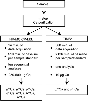Fig. 1 Schematic of the applied approach to measure the mass-independent (μ⁴⁰Ca, μ⁴³Ca, μ⁴⁶Ca, and μ⁴⁸Ca), as well as the mass-dependent (δ⁴²Ca, δ⁴³Ca, δ⁴⁶Ca, and δ⁴⁸Ca) Ca isotope composition of a single sample.

2 Analytical methods

2.1 Standard, samples and sample digestion

In contrast to most previous studies that used SRM 915a as Ca standard, all measurements here are reported relative to the SRM 915b standard obtained from the National Institute of Standards and Technology (NIST), given that SRM 915a is no longer supplied by NIST and has been superseded by SRM 915b. Moreover, the mass-dependent Ca isotopic composition of SRM 915b is much more representative for bulk silicate Earth than its predecessor,¹³ which is highly desirable when searching for nucleosynthetic anomalies. A batch of 400 mg of SRM 915b was dissolved to ensure homogeneity of the standard. The single largest contaminant element in SRM 915b is Sr at a concentration of 150 μg g⁻¹. At this level, Sr does significantly affect the accuracy of the HR-MC-ICPMS analysis. Therefore SRM 915b aliquots were taken from the large dissolution, processed through step 1 (see below) of the Ca purification applied to all samples and checked for any remaining Sr before being used as standards for analysis.

In order to test the robustness of the new and highly-precise method for Ca isotope measurements presented here, a total of seven terrestrial rock standards and the OSIL Atlantic Seawater Conductivity Standard were analyzed relative to SRM 915b. In detail, we analyzed the two Hawaiian basalts BHVO-1 and BHVO-2, the Columbia River flood basalt sample BCR-2, an olivine-normative dolerite (DNC-1) and the icelandic dolerite BIR-1. These samples were accompanied by SGR-1, a shale from the Green River formation, and SARM 40, a South African carbonatite. With the exception of SARM 40 all rock standards were obtained from the United States Geological Survey. SARM 40 was provided by the South African Bureau of Standards. In order to allow better comparison of our data with data published elsewhere we also measured an aliquot of SRM 915a Ca standard. Generally between 20 and 50 mg of rock powder were processed for each sample. Rock powders were digested in Savillex beakers containing a 1 : 1 mixture of concentrated HF-HNO₃ at 210 °C under high pressure in a Parr bomb for three days. After digestion samples were evaporated to dryness and redissolved twice with 6 M HNO₃ and one time in 6 M HCl to ensure complete dissolution. Following this, samples were dried down and converted to nitric form for chemical Ca purification.

2.2 Ca purification

Calcium is typically separated from the sample matrix using cation exchange resin chemistries^8,13 sometimes accompanied by a specific Ca-Sr separation step with Sr-specific resin.^11,14 Russel and Papanastassiou¹⁵ demonstrated that loss of Ca during cation-exchange column chemistry with Dowex-50 resin can result in a strong isotopic fractionation. For isotopic analyses where the mass-dependent effects of Ca are of interest, such fractionation can be counteracted through the use of a double-spike. However, the technique we developed is aimed at describing both mass-dependent and mass-independent effects on Ca isotopes and, thus, we cannot use a double-spike approach. As such, care must be taken to ensure adequate recovery during Ca purification. Moreover, the presence of residual sample matrix can potentially affect the accuracy of Ca isotope data because of irresolvable direct isobaric interferences (i.e., ⁸⁶Sr²⁺, ⁸⁸Sr²⁺, ⁴⁶Ti⁺ and ⁴⁸Ti⁺) or, alternatively, uncorrectable mass fractionation effects.^16,17 In order to minimize the matrix component in purified Ca cuts, all chemical separation steps were designed to function as on-off separation steps that behave independently of the sample matrix used, and do not require a precise calibration to avoid loss of Ca.

While this approach is slightly more cumbersome than separation techniques used in previous studies, the four step chemistry (Table 1) applied here ensures 99.9% recovery. It also provides a very high level of Ca purification and excellent separation of Ca from elements that may create direct isobaric interferences (e.g., ²⁴Mg¹⁶O⁺ and ²⁷Al¹⁶O⁺) and/or affect the instrumental mass fractionation as compared to the standard during analysis. Importantly, the Sr/Ca and Ti/Ca ratios are less than 1 : 1,000,000 after the full chemistry and do not affect data accuracy at a resolvable level. Total procedure blanks were a few ng of Ca and are negligible compared to the total amount of Ca typically processed (∼1 mg). After the purification samples were first measured with the HR-MC-ICPMS, an aliquot of the remaining sample was used for Ca isotope analysis by TIMS.

Table 1 Four step Ca purification scheme

Eluent	Vol.^a	Elements eluted
a Volume of eluent. b 3 cm long column made from a 1 mL squeeze pipette with 200 μL Eichrom Sr-spec resin. c 1.5 mL pipette tip column with 0.5 mL AG1-X4 200–400 mesh resin. d Biorad-type column with 2 mL of TODGA resin.^18,19 e Biorad-type column with 1 mL of BioRad AG50W-X8 200–400 mesh resin.
Step 1: Sr-separation ^b
2 M HNO3	2	Conditioning
Load sample in 2 M HNO3	1
2 M HNO3	2	Ca + matrix
remaining on column		Sr, Ba
Step 2: Fe-clean up ^c
6 M HCl	2	Conditioning
Load sample in 6 M HCl	1
6 M HCl	2	Ca + matrix
remaining on column		Fe
Step 3: matrix removal ^d
2 M HNO3	4	Conditioning
Load sample in 2 M HNO3	1
2 M HNO3	4	matrix
15 M HNO3	5	Ca ± Ti
Step 4: Ti clean up ^e
1 M HNO3 + 0.1 M HF	5	Conditioning
Load sample in 1 M HNO3 + 0.1 M HF	1
1 M HNO3 + 0.1 M HF	4	Ti, Sr, Na
6 M HNO3	10	Ca

---

A potential hazard in the Ca purification is the use of trace amounts of hydrofluoric acid in the last chemical separation step, because of the possibility of CaF₂ precipitation. No such loss was observed through decreased Ca yields or fractionation of column processed Ca standard (Table 2 and 3). It should also be noted that the upper limit of Ca processed through this purification step at any time was less than 1 mg mL⁻¹, while at room temperatures the solubility of CaF₂ in 1 M HNO₃ is in excess of 2 mg mL⁻¹ and increases toward 6 M HNO₃ to about 6 mg mL⁻¹.²⁰

Table 2 Stable Ca isotope composition of various standards relative to SRM 915b measured using the Neptune Plus HR-MC-ICPMS. Data from other sources is shown for comparison. SRM 915b cp. has been processed alongside the samples through the full chemistry. The reported uncertainties are two times the standard error of ten sequential analyses within a single session lasting up to 22 h

Sample	Material/Literature Ref.	δ^42Ca	δ^43Ca	δ^46Ca	δ^48Ca
BCR-2	basalt	–0.08 ± 0.04	–0.04 ± 0.02	+0.17 ± 0.06	+0.17 ± 0.08
	Wombacher et al.^13	–0.10 ± 0.10
	Amini et al.^5	–0.08 ± 0.04
BHVO-1	basalt	–0.08 ± 0.03	–0.04 ± 0.02	+0.06 ± 0.04	+0.14 ± 0.06
BHVO-2	basalt	–0.04 ± 0.04	–0.02 ± 0.02	+0.06 ± 0.04	+0.09 ± 0.07
	Amini et al.^5	–0.06 ± 0.04
BIR-1	dolerite	–0.04 ± 0.03	–0.01 ± 0.02	+0.05 ± 0.04	+0.05 ± 0.07
	Wombacher et al.^13	–0.05 ± 0.05
	Amini et al.^5	–0.03 ± 0.05
DNC-1	dolerite	–0.04 ± 0.03	–0.02 ± 0.01	+0.02 ± 0.04	+0.07 ± 0.06
SARM 40	carbonatite	–0.08 ± 0.02	–0.04 ± 0.01	+0.07 ± 0.04	+0.16 ± 0.04
av. igneous rocks		–0.06 ± 0.02	–0.03 ± 0.01	+0.07 ± 0.04	+0.11 ± 0.04
SGR-1	shale	–0.02 ± 0.02	–0.01 ± 0.01	+0.00 ± 0.05	+0.03 ± 0.05
	Wombacher et al.^13	–0.07 ± 0.07
OSIL AL	seawater	–0.53 ± 0.02	–0.26 ± 0.01	+0.50 ± 0.02	+0.98 ± 0.03
	Wombacher et al.^13	–0.58 ± 0.08
SRM 915b cp.	carbonate	–0.04 ± 0.03	–0.02 ± 0.01	+0.01 ± 0.04	+0.09 ± 0.04
SRM 915a	carbonate	+0.42 ± 0.02	+0.20 ± 0.01	–0.29 ± 0.03	–0.72 ± 0.05
	Wombacher et al.^13	+0.36 ± 0.03
	Heuser et al.^23	+0.36 ± 0.02

---

Table 3 Mass-bias corrected Ca isotope data (using a constant ⁴²Ca/⁴⁴Ca = 0.31221²) for various standards measured relative to SRM 915b by Neptune Plus HR-MC-ICPMS (μ⁴³Ca, μ⁴⁶Ca and μ⁴⁸Ca). The reported uncertainties are two times the standard error of ten sequential analyses within a single session lasting up to 22 h

Sample	μ^43Ca	μ^46Ca	μ^48Ca
BCR-2	–1.0 ± 1.7	+27.5 ± 42.4	+5.2 ± 3.4
BHVO-1	–1.1 ± 1.4	–37.0 ± 34.0	–6.1 ± 8.1
BHVO-2	–2.0 ± 2.3	–0.3 ± 17.0	+6.3 ± 7.5
BIR-1	–1.3 ± 1.6	+31.4 ± 25.2	+6.1 ± 5.7
DNC-1	–0.3 ± 1.5	–4.3 ± 29.2	+1.0 ± 4.0
SARM 40	–0.2 ± 2.4	–23.0 ± 24.0	–6.7 ± 9.7
SGR-1	+0.1 ± 1.2	–6.0 ± 30.0	–4.6 ± 8.7
OSIL AL	+0.1 ± 2.1	–17.6 ± 8.5	–10.7 ± 7.9
average	–0.7 ± 0.7	–5 ± 15	–0.4 ± 4.6
SRM 915a	–5.5 ± 0.8	+107.0 ± 11.0	+62.7 ± 6.1
SRM 915b cp.	–1.6 ± 1.0	–18.0 ± 10.0	+3.4 ± 6.3

---

2.3 Ca isotope measurements by HR-MC-ICPMS

The Ca isotopes, excluding ⁴⁰Ca, were measured using the ThermoFisher Neptune MC-ICPMS located at the Centre for Star and Planet Formation (Natural History Museum of Denmark, University of Copenhagen). Following Ca purification samples were dissolved in a 2% HNO₃ solution and introduced into the plasma source by means of an ESI Apex IR desolvating nebulizer combined with an ESI ACM (temperature stabilized membrane desolvator) attachment. Samples were aspirated at a rate of approximately 0.130 mL min⁻¹. Optimal signal stability and sensitivity was typically achieved with a sample gas flow rate of 850 mL min⁻¹ and a sweep gas pressure of 1.5 bar for the ACM.

Calcium isotope data were acquired in static mode using six Faraday collectors (Fig. 2). All measurements were made in high-resolution mode either using the 30 and 16 μm entrance slit with a resolving power (M/ΔM as defined by the peak edge width from 5–95% full peak height) that was always greater than 5,000. Prior to each analytical session, ⁴²Ca/⁴⁴Ca, ⁴³Ca/⁴⁴Ca, ⁴⁶Ca/⁴⁴Ca, ⁴⁷Ti/⁴⁴Ca and ⁴⁸Ca/⁴⁴Ca ratios were measured at different positions on the left-hand side of the Ca peak to define an interference-free flat plateau (Fig. 3). Ca isotope data were then acquired on this plateau, typically located 0.024 a.m.u. from the center of the Ca peak. The measurement position on this plateau corresponds to an effective mass resolution of about half the resolving power, thereby allowing for the resolution of the most prominent of the various interferences on Ca isotopes on the high-mass side. Importantly, the torch related and unavoidable ²⁸Si¹⁴N⁺ and ²⁸Si¹⁶O⁺ interferences on the ⁴²Ca and ⁴⁴Ca beams, which are used for mass fractionation correction of the other Ca isotopes, were fully resolved.

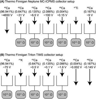Fig. 2 Shown in (A) is the collector setup used with the Neptune MC-ICPMS and in (B) the collector setup used with the Triton TIMS. Apart from ⁴⁰Ca, all Ca isotopes were measured by HR-MC-ICPMS. For TIMS analyses, the ⁴⁰Ca to ⁴⁴Ca were measured ignoring the small ⁴⁶Ca and ⁴⁸Ca beams. ⁴¹K was used to correct for ⁴⁰K. The natural abundance of each isotope, the respective amplifier used for each faraday cup and typical voltages measured during a sample analysis are indicated for each isotope.

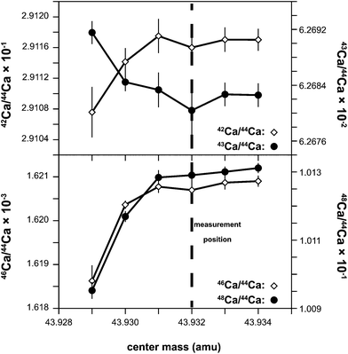Fig. 3 Shown are the ^42/44Ca, ^43/44Ca, ^46/44Ca, and ^48/44Ca ratios measured at six different positions on the low mass side of the ⁴⁴Ca peak relative to the peak center. This was used to test the alignment of the Ca isotope peaks and determine an interference-free flat top peak for isotopic analysis.

The sensitivity of the instrument under these analytical conditions and depending on the entrance slit used was between 300–800 V ppm⁻¹. Samples and standards were analyzed with a signal intensity of approximately 100 V on mass ⁴⁴Ca, corresponding to a total signal strength of ∼5,000 V for a solution with a concentration of ∼8–16 ppm. Each analysis comprised a total of 839 s of data acquisition (100 scans integrated over 8.39 s). Prior to each analysis up to 2391 s of on-peak data were measured in a blank solution. After offline data scrutinization for a clean baseline signal using Iolite,²¹ the last 600–1,000 s of this data were typically used for baseline correction (Fig. 4). A peak center was conducted before each standard analysis. Sample analyses were bracketed by analyses of SRM 915b standard to monitor instrumental mass fractionation. Each sample was systematically analyzed 10 times and the reported isotopic compositions are an average of these. This corresponds to a total of ∼250 to 500 μg of Ca consumed for each sample in a single session typically lasting up to 22 h. No adjustment of the tuning parameter was done for the duration of such a session. Due to the high beam intensities used for the analysis, the instrument sensitivity generally degraded by 20–30% throughout the measurement sequence of a single sample. The cause for this is coating of Ca on the skimmer X-cone. Cleaning the X-cone prior to each sample analysis efficiently counteracted this problem.

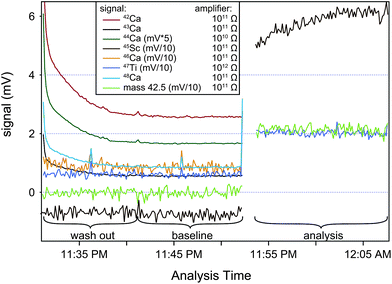Fig. 4 Shown is a typical wash-out and baseline measurement of the masses ⁴²Ca, ⁴³Ca, ⁴⁴Ca, ⁴⁵Sc, ⁴⁶Ca, ⁴⁸Ca, ⁴⁷Ti and 42.5. Also shown are the signals at masses ⁴⁵Sc, ⁴⁷Ti and 42.5 for a typical sample/standard analysis. To facilitate comparison of all beams, signals for ⁴⁵Sc, ⁴⁶Ca, ⁴⁷Ti and mass 42.5 are shown increased by a factor of ten and the signal for ⁴⁴Ca has been scaled down by a factor of 5. Elevated signals during analysis of ⁴⁷Ti and mass 42.5 are due to signal scattering of the ⁴⁰Ca beam, the ⁴⁵Sc signal is a combination of real scandium blank as well as ⁴⁰Ca beam scattering and ⁴⁴Ca¹H⁺ from a ca. 77 V ⁴⁴Ca signal.

2.4 Ca isotope measurements by TIMS

Following HR-MC-ICPMS analyses, the lower mass range of Ca isotopes (⁴⁰Ca, ⁴²Ca, ⁴³Ca, and ⁴⁴Ca) were analyzed on the same sample with the ThermoFisher Triton TIMS located at the Centre for Star and Planet Formation, using a double filament technique. About 10 μg Ca was loaded onto a zone refined Re filament in 2 μL of 6 M HCl. The solutions were dried onto the filament at an applied current of ∼0.6 A. After dry down, the current was slowly increased to ∼1.8 A and kept at this level for about 30 s. To avoid potential rehydration of Ca at atmospheric conditions, we have ensured that the filament holding turret was inserted into the TIMS sample chamber immediately after loading was completed.

Calcium isotope data were acquired in static mode using five Faraday collectors (Fig. 2). The ionizing and evaporation filaments for samples and standards were heated-up at 450 mA min⁻¹ and 150 mA min⁻¹, respectively. Data acquisition was typically initiated when currents of 4,500 mA and 1,200 mA were applied to the ionizing and evaporation filaments, respectively, which resulted in a recorded pyrometer temperature of ∼1,700 °C. The adjustment to the evaporation filament current was always less than 100 mA throughout an analytical session and no filament was run to exhaustion. A filament loaded with SRM 915b was analyzed prior and after each sample analysis.

In contrast to the common approach where baselines are collected in short intervals during the sample analysis while the filament is hot and sample is evaporating, a single, long baseline was collected in advance of the sample analysis before any filament current was applied. Baseline measurements were conducted as ‘on peak zero’ measurements identical to a sample analysis except the lack of filament current, peak centering and beam focussing. Baseline data were acquired for at least 4 blocks of 244 cycles of 8.39 s or a total of 136.6 min. Sample analysis consisted of 200 block with 20 8.39 s cycles per block or a total of 560 min. Blocks were kept short to allow for regular adjustment of the evaporation filament current to hold a constant signal. Lens focus was conducted every 10 blocks, filament focus every 20 blocks and a peak center was conducted every 40 blocks.

2.5 Data reduction

All data reduction was conducted off-line using the freely available Iolite²¹ data reduction software (http://iolite.earthsci.unimelb.edu.au/) that runs within Igor Pro. Both Ca data reduction modules used for Ca isotope ratio calculations can be freely obtained from the authors on request.

2.5.1 Neptune HR-MC-ICPMS data reduction. Both changes in mass fractionation and baseline intensities were interpolated using the ‘spline smooth auto’ choice. This spline is a smoothed cubic spline that determines the optimal degree of smoothing based on variability in the reference standard throughout an analytical session.²² This corresponds to 11 standard measurements over ∼22 h with no adjustments of the tuning parameters.

The on-peak zero measurements were screened for the appropriate washout time where no significant decrease in the baseline was observed on any collector. This typically resulted in 600–1,000 s of baseline measurement collected prior to each analysis, which was subjected to a 2 sd outlier rejection scheme. The mean and standard error of all sample and standard analysis was calculated with a 2 sd outlier rejection scheme. Sample analyses of a single sample in one session (n = 10) were combined weighted by the propagated uncertainties on single analysis to produce an average. All mass-dependent Ca isotope data are reported relative to the composition of SRM 915b^13,23 in the δ (per 10³ deviation) notation:

where x = 42, 43, 46, or 48. The mass-independent component of ⁴³Ca, ⁴⁶Ca, and ⁴⁸Ca is reported in the μ (per 10⁶ deviation) notation because this reflects more closely the precision achieved in this study. Instrumental mass fractionation was corrected with the exponential law, normalizing to a constant ⁴²Ca/⁴⁴Ca = 0.31221²

Internal errors for single analysis of δ⁴²Ca, δ⁴³Ca, δ⁴⁶Ca, and δ⁴⁸Ca (2 se) were typically 10–30, 10–20, 25–50, and 30–60 ppm, respectively. Pooling the data over 10 analyses results in weighted means with typical uncertainties (2 se) of 0.02–0.05, 0.01–0.03, 0.02–0.06, and 0.03–0.1‰ for the δ⁴²Ca, δ⁴³Ca, δ⁴⁶Ca, and δ⁴⁸Ca, respectively (Table 2), which include the uncertainty associated with the standard spline. The variability of the internal errors for the mass-dependent isotope data is mainly caused by changes of the mass fractionation within a single analysis related to Ca coating the sampler and skimmer cone and/or small fluctuations in the sample uptake rate. After mass fractionation correction single analysis of μ⁴³Ca, μ⁴⁶Ca, and μ⁴⁸Ca have uncertainties of 5–7, 20–40, and 10–20 ppm resulting in final uncertainties of a complete session of 1.0–2.4, 8.5–42.4, and 3.4–9.7 ppm, respectively (Table 3). The final error of the mass fractionation corrected data is mainly influenced by the total signal intensity, signal stability throughout the run, length of time between peak centers and the magnet stability over this time, as well as stability of the tune settings (mainly the nitrogen and sample gas interplay).

2.5.2 Triton TIMS data reduction. Baseline intensities were interpolated in the same manner as for the MC-ICPMS data reduction using the ‘spline smooth auto’ option of Iolite to fit a spline through all baseline measurements of a single session. This corresponds to a fit through 21 baseline measurements of at least 2.5 h each over a period of 14 to 17 days. ⁴⁰Ca/⁴⁴Ca and ⁴³Ca/⁴⁴Ca ratios were corrected for mass fractionation using the generalized power law²⁴ and a ⁴²Ca/⁴⁴Ca = 0.31221. The exponent for the generalized power law was determined for each session separately (for details see below) and was close to a kinetic law with a modest equilibrium contribution. The isobaric ⁴⁰K interference on ⁴⁰Ca was corrected using the mass fractionation corrected ⁴¹K intensity, and was typically less than 0.3 ppm. Samples are reported as the relative deviation from a linear fit through all measurements of the SRM 915b standard measured on the same turret bracketing each sample analysis. Only standards from the same session were used to report against to ensure that both, standards and samples, were measured under the same analytical conditions (i.e. the same gain calibration). The reported error is the estimated reproducibility based on the 2 sd of all SRM 915b standard measurements (n = 26) measured throughout the course of this study. Internal errors of single analyses were typically 4.5 (μ⁴⁰Ca) and 5.5 ppm (μ⁴³Ca).

3 Results and discussion

3.1 Neptune HR-MC-ICPMS sample introduction and cup alignment

There are two major obstacles in obtaining highly-precise and accurate mass-independent data for Ca isotopes by MC-ICPMS. First, it is essential to measure all isotopes in a Poisson noise dominated regime, which corresponds to a signal intensity greater than 100 mV for the ⁴⁶Ca when measured with a 10¹¹ Ω feedback resistor.²⁵ Given the low abundance of ⁴⁶Ca, this would result in a total Ca beam of 3,000 V, which is not possible to measure using state-of-the-art amplifiers. To overcome this problem, we chose not to measure the ⁴⁰Ca beam (or 97% of the total beam intensity); this allows to significantly improve the precision of the measurements for the remaining Ca isotopes. Second, it is necessary to minimize or resolve the abundant gas-based interferences on the Ca mass array and ⁴⁷Ti. This requires that analyses are conducted in high-resolution mode, which reduces sensitivity by a factor of five to ten. In order to compensate for this loss of sensitivity, we use an ESI Apex IR desolvating nebulizer sample introduction system, including the ACM attachment. The typical sensitivity of the instrument using this sample introduction system is ∼300–800 V/ppm, depending on uptake rate and resolution slit used.

The ESI Apex IR was preferred over other desolvating nebulizers such as, for example, the Cetac Aridus II, because the quartz flow path of the Apex provides better wash outs compared to other systems. Moreover, when combined with the ACM unit, the ESI Apex IR allows for improved signal stability despite the constant high ion load of the sample solutions (5–16 ppm), which made it ideally suited for the time intensive measurements of this study. Apart from an improved signal stability, the use of the ACM unit lowers oxide and hydride production. This is important because the high-sensitivity sample and skimmer cones used here can also result in an enhanced production of oxides and, possibly, hydrides.²⁶

Because Ca-hydrides cannot be resolved at the applied mass resolution, we have taken care of estimating the hydride production during individual measurements by monitoring the ⁴⁵Sc signal. Assuming the ⁴⁵Sc signal is purely Ca-hydride, we show in Fig. 4 that a ∼77 V ⁴⁴Ca signal produced 600 μV of ⁴⁴Ca¹H⁺, corresponding to a hydride production rate of ca. ∼8 ppm. Based on this estimation, we determine the potential hydride contribution at masses ⁴³Ca and ⁴⁴Ca to be 18 ppm and 0.5 ppm of the total signal. Although this is insignificant for ⁴⁴Ca, the potential effects on mass ⁴³Ca signal requires the signal intensity of standard and sample to be matched within 15% or better to avoid a systematic offset of the mass fractionation corrected data outside the typical analytical uncertainty. To avoid this pitfall, sample and standard Ca solutions were always adjusted to have concentration within <2% of each other.

The high Ca concentrations resulted in a fast degradation of the sensitivity of the machine. This was caused by Ca depositing on the skimmer and sampler cones. As mentioned above, this effect was counteracted by cleaning both cones after each sample analysis in 0.2% nitric acid in an ultrasonic bath for 15 min to redissolve any deposits. An unwanted side-effect of this regular cone cleaning, however, is initial large drift in the uncorrected raw ratios at the beginning of each session while the cones receive an initial coating. During this initial drift, which can last up to ∼1 h of signal time, the instrumental mass fractionation can be different from the remainder of the session. Generally this problem was avoided by conditioning the cones during the tuning of the machine.

Another significant problem of the high beam intensities is the high wear on beam focussing parts of the Neptune. Degradation of the resolution slit caused by the beam required that the slits were changed after 5 to 7 samples (or about 150 h of continuous measurement) to maintain a sufficiently high resolving power needed for to resolve interferences. Due to deformation and erosion caused by the beam, both the entrance slit and the aperture lens had to be replaced during the course of this study. The replacement of these two lenses was important because wear on these lenses allows a more intense beam to reach the resolution slits further decreasing their lifetime.

It was not possible to avoid elevated signal noise due to beam scattering of the large ⁴⁰Ar and ⁴⁰Ca beams on the Ca mass array.²⁷ To assess the impact of beam scattering, we monitored signal intensities between masses 42 and 43 as well as between masses 47 and 48 with faraday detectors connected to 10¹¹ Ω feedback resistors. Both detectors showed increased signal intensities up to 300 μV during analysis relative to the washout sequences. Our data also shows that the scattering effect scales with Ca signal intensity (Fig. 5) linking it directly to the Ca beam intensity. The largest scatter signal of 300 μV was observed at a 30 V ⁴²Ca beam, which equates to a potential 10 ppm effect on ⁴²Ca. However, because the scatter signal correlates with beam intensity, it is possible to minimize the potential inaccuracies caused by scattering by closely matching the signal intensities of standard and sample.

Fig. 5 Correlation of the ⁴²Ca beam with the signal intensity measured at mass 42.5 during an analytical session of BHVO-2 measured versusSRM 915b. The fit shown is based on: y = a + b*e^(−c*x), where: a = 0.00013817, b = −0.0019117, and c = 0.20325.

3.2 Ti correction for ⁴⁶Ca and ⁴⁸Ca (Neptune)

Both ⁴⁶Ti (8.25%) and ⁴⁸Ti (73.72%) directly interfere with the ⁴⁶Ca and ⁴⁸Ca measurements, respectively. These interferences provide a special challenge for the precise and accurate measurement of ⁴⁶Ca, which has a natural abundance of only about 0.003%. The significant difference in natural abundance of ⁴⁶Ca and ⁴⁶Ti equates to about 2,000 times more ⁴⁶Ti than ⁴⁶Ca and ca. 400 times more ⁴⁸Ti than ⁴⁸Ca in a 1 : 1 Ti:Ca solution. These large ratios illustrate that even small amounts of residual Ti can result in an interference correction of hundreds of ppm. Considering the precision of ⁴⁶Ca reported here (45 ppm), insufficient or incorrect interference corrections can therefore potentially have a severe effect on the accuracy of the results.

To test for the effects of incorrect mass fractionation correction of Ti, an Aristar Ca doped with about 0.24% Ti was measured versus an undoped solution. Prior to Ti interference correction μ⁴⁶Ca and μ⁴⁸Ca anomalies in this experiment were +128,000 and +20,000 ppm, respectively. After interference correction residual anomalies were +635 and −104 ppm showing an imperfect interference correction at this level of Ti in the sample. However, due to the rigorous chemical purification Ti concentrations were more than 1,000 times lower, resulting in μ⁴⁶Ca corrections for samples that were 200 ppm or less. At this level, incorrect mass fractionation correction of the Ti signal is estimated to be at the sub-ppm level for each isotope and well below the external reproducibility.

To ensure such low levels of interference corrections, samples were screened prior to analysis for their Ti concentrations. However, because of the large ⁴⁰Ca signal scattering precise absolute measurement of the ⁴⁷Ti was impossible with the faraday collectors. To avoid this problem, we also measured ⁴⁷Ti intensities in most samples to better gauge ⁴⁷Ti signal intensities using a secondary electron multiplier with a retarding potential quadrupole filter (RPQ-SEM). ⁴⁷Ti signals for samples analyzed at 100 V of ⁴⁴Ca signal were generally less than 20,000 counts per second. Samples with larger ⁴⁷Ti signals were reprocessed through the fourth Ca cleaning step for further purification. In general, this additional step was sufficient to reach an adequate purity for all samples reported here.

3.3 Separate baseline—sample measurements—Triton TIMS

The typical strategy for baseline measurements by TIMS is to acquire data over relatively short time periods (60–300 s) at the beginning of each block of data while the sample is evaporating on a hot filament, either using a defocussed beam or, alternatively, by measuring at the half mass. However, this approach may not be advantageous when sample limited, given that a significant part of the sample analysis routine is spent measuring baselines instead of acquiring isotope data. This problem is further amplified when acquiring isotope data with relatively low signal intensities (i.e., <100 mV), as the length of the baselines measurements can be extended to nearly 50% (e.g., ref. 25) of the sample analysis time to ensure an adequate signal to noise ratio. Clearly, such a strategy hampers the final precision of individual measurements, especially when sample limited. Therefore, we have elected to measure baselines independently of the sample analysis, that is, similarly to routines developed for isotope measurements by MC-ICPMS. In detail, we conducted baseline measurements prior to and after each analysis under similar conditions as the analysis. The only difference between a baseline and sample analysis was that no filament current was applied during the baseline measurement. Single baselines last typically between 2.4 to 5 h. Baseline correction was applied offline using a spline fit through all baseline measurements conducted within the same session. This was done based on the assumption that there is no uncorrected short term drift within a few hours while long term drift of during the timescale of a single session of multiple days can be accounted for by regularly spaced baseline measurements.

The validity of this approach can be investigated by examining the signal behavior of the baseline measurements over multiple hours such as shown in Fig. 6 as well as the variability of these baseline measurements over multiple days (Fig. 7). Signal variability during the course of a single baseline measurement over multiple hours (Fig. 6) allows to quantify signal stability over such timescales. The 10¹¹ Ω amplifiers used in this study have a variability in the baseline signal of <0.5 μV (2 se) over short periods of time (5 h) and the 10¹⁰ Ω amplifier of 1.6 μV (2 se). In agreement with the change in resistivity, signal variability of the 10¹⁰ Ω amplifier is larger by a factor of 10 than that of 10¹¹ Ω amplifiers. This indicates that there is no systematic drift that is larger than their noise levels in either of the amplifiers. However, we identified and excluded a 10¹¹ Ω amplifier of the Copenhagen Triton that exhibited jumps in the signal baseline that lasted up to several hours based on such baseline measurements. This behavior would have not been identifiable with short baselines during the duration of a sample analysis and also could not have been eradicated by amplifier rotation. Over the timespan of 14 days the signal variability of each 10¹¹ Ω amplifier ranges from 3.4 to 4.3 μV (2 sd, n = 20) and is 30 μV for the 10¹⁰ Ω amplifier. This long term drift over multiple days is modeled by a spline fit that allows to correct any baseline drift between separate baselines. The lack of a resolvable systematic short term drift in the baselines (Fig. 6) suggests that the approach taken here is well suited to increase the measured ion yield from a single sample filament while also being able to measure very long baselines. In addition, the long term stability and the lack of significant drift of the amplifier baselines supports our approach of measuring regularly long baselines and using a single gain calibration throughout a single session.

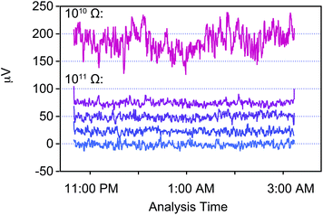Fig. 6 An example of the signal variability throughout a single Ca isotope baseline measurement by TIMS over approximately 4.6 h. Shown are the variations in signal intensity measured for each cup used for the Ca measurement connected to a 10¹⁰ Ω (⁴⁰Ca) and four 10¹¹ Ω (⁴¹K, ⁴²Ca, ⁴³Ca, and ⁴⁴Ca) amplifiers as a running average of ten measurements. Measurements were done on-peak with the gate valve open during the measurement with no filament current applied. The relative intensities are to scale, whereas absolute intensities have been shifted to allow for better comparison. The internal errors (2 se) over the 4.6 h period for these baselines are 1.6 μV (10¹⁰ Ω) and <0.5 μV for the 10¹¹ Ω amplifiers.

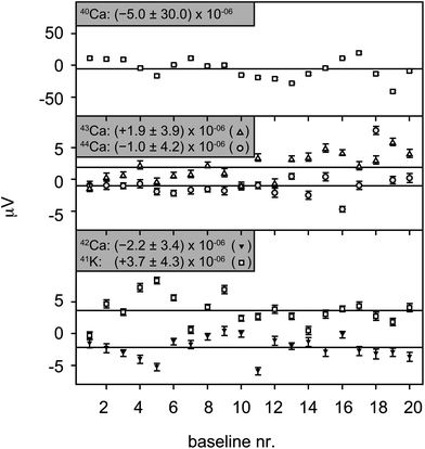Fig. 7 Long term variability of the baseline measurements by TIMS shown for each measured mass separately. The uncertainties for each of the masses are the 2 sd of 20 baselines measured in a single 14 day session with the same gain calibration. Single baselines were measured for 2.4 to 4.6 h, and the uncertainties are the 2 se for each analysis.

3.4 Correction of instrumental mass fractionation

The use of the appropriate mass fractionation law to correct for natural and instrumental mass fractionation is critical to achieve precise and reproducible results. Our data obtained for Ca, both from the Neptune and Triton, show that the kinetic law generally used to correct for mass fractionation is not entirely accurate in describing the true instrumental mass fractionation of these measurements (Fig. 8 and 9). Instead, under stable running conditions (after initial cone conditioning) we observe a mass fractionation for Ca measured with the Neptune MC-ICPMS that closely follows the power law (Fig. 8). A similar effect has previously been observed for Mg isotopes using the same instrument, but with a different sample introduction system and sampler cone.²² Based on this observation, it does not appear that the new Jet cone used in this study or the Apex sample introduction system have any significant influence on the mass fractionation of the machine. Despite the observed power law relationship, however, we use the kinetic law to correct for instrumental mass fractionation of the MC-ICPMS. This is based on the assumption that the kinetic law more likely represents mass-dependent fractionation that occurs in nature. This is important for samples that have a distinct mass-dependent isotopic composition from the standard. In such a case, wrong mass fractionation correction can yield apparent mass-independent effects. Here, we minimize this potential pitfall by using SRM 915b which has a mass-dependent isotopic composition that is closely matched to BSE (Table 2). Because of the long term stability of the mass fractionation of the MC-ICPMS, mass fractionation effects due to incorrect mass fractionation correction of mass fractionation occurring in the machine itself can be negated by standard sample bracketing.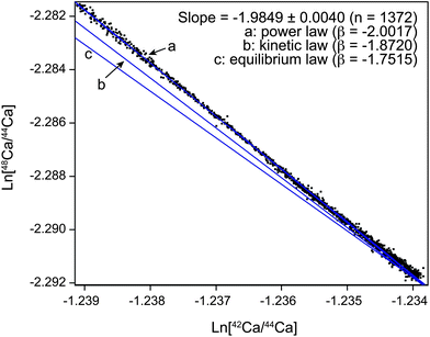

Fig. 8 Ca three isotope diagram illustrating the mass fractionation during a sample run using the Neptune Plus HR-MC-ICPMS with an Apex IR with attached ACM module. Shown are the natural logarithms of 1,372 raw ⁴²Ca/⁴⁴Ca and ⁴⁸Ca/⁴⁴Ca ratios measured as 8.39 s integrations in a single session of 13 h. Also indicated are the expected slopes for mass fractionation that follows a) power, b) kinetic, c) equilibrium type mass fractionation.

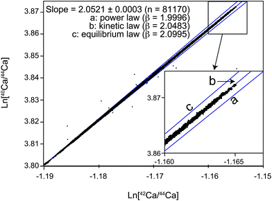Fig. 9 Ca three isotope diagram illustrating the mass fractionation using TIMS with Ca loaded in HCl on a double filament setup. Shown are the natural logarithms of 81,170 raw ⁴⁰Ca/⁴⁴Caversus⁴²Ca/⁴⁴Ca ratios measured as 8.39 s integrations in a single session of ca. 14 days. Also indicated are the expected slopes for mass fractionation that follows a) power, b) kinetic, c) equilibrium type mass fractionation.

The use of the correct mass fractionation law is much more critical for the TIMS, where elemental mass fractionation is changing with time. In agreement with our data, Hart and Zindler²⁸ recognized that Ca mass fractionation can be closely described by the exponential law, although there are observable discrepancies they ascribed to reservoir mixing effects (Fig. 9). In an attempt to reduce scatter in the data resulting from an imperfect mass fractionation correction, we corrected our data using the general power law instead of the exponential law. Treating each analytical session individually, we determined the most appropriate exponent by minimizing the Pearson's correlation coefficient between measured ^42/44Ca and mass fractionation corrected ^40/44Ca ratios for all standards. For the 3 individual sessions during which data was acquired, the β ranged from −0.095 to −0.172, where β of 0 is equivalent to the exponential law and −1 to the equilibrium law. The use of the optimized generalized power law resulted in an improved external reproducibility of the mass fractionation corrected ^40/44Ca by about 10% compared to a correction using the kinetic law. The remaining variability between standards is mostly a result of fractionation effects within a single analysis that cannot be corrected for using the same correction for each sample.

3.5 Reproducibility and comparison with published data

3.5.1 Accuracy and reproducibility of mass-independent data. The limitations to the precision of the mass fractionation corrected isotope data are different for the TIMS and the MC-ICPMS (Fig. 10). This is most obvious for μ⁴³Ca, which has been determined using both techniques. Using the TIMS, the external reproducibility of our data set for μ⁴⁰Ca_TIMS and μ⁴³Ca_TIMS is 80 and 23 ppm, respectively (Table 4). In contrast, the external reproducibilities of the MC-ICPMS data for μ⁴³Ca_MC-ICPMS, μ⁴⁶Ca_MC-ICPMS, and μ⁴⁸Ca_MC-ICPMS are 1.8, 45 and 12.5 ppm, respectively (Table 3).

Table 4 Mass-bias corrected Ca isotope data (using a constant ⁴²Ca/⁴⁴Ca = 0.31221²) for various standards measured relative to SRM 915b by Triton TIMS. Also shown are the measured absolute ⁴⁰Ca/⁴⁴Ca ratios. Where not stated otherwise, each reported value represents a single analysis. The reported uncertainties are the estimated external reproducibility of the method based on the 2 sd of all SRM 915b standard measurements

Sample	μ^40CaTIMS	μ^43CaTIMS	^40/ ^44Ca
BCR-2	+3 ± 80	–3 ± 23	47.1645
BHVO-1	–43 ± 80	+9 ± 23	47.1623
BHVO-2	–88 ± 80	+9 ± 23	47.1602
BIR-1	–124 ± 80	–20 ± 23	47.1585
DNC-1	–126 ± 80	–17 ± 23	47.1584
SARM 40	–34 ± 80	+15 ± 23	47.1633
SGR-1	–39 ± 80	+24 ± 23	47.1635
OSIL AL	–102 ± 80	+16 ± 23	47.1601
average (n = 8)	–69 ± 35	+4 ± 11
SRM 915a (n = 3)	+5 ± 28	+1 ± 10	47.1662 ± 0.0023
SRM 915a^6			47.1525 ± 0.0074
SRM 915a^10			47.1622 ± 0.0016
SRM 915b (n = 26)			47.1645 ± 0.0038

---

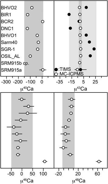Fig. 10 Mass bias corrected isotope data for various rock standards. μ⁴⁰Ca and μ⁴³Ca are mass fractionation corrected TIMS data and μ⁴³Ca, μ⁴⁶Ca and μ⁴⁸Ca are mass fractionation corrected MC-ICPMS data. Grey bars represent the 2 standard deviation of the rock standards. For μ⁴³Ca both datasets, obtained with the TIMS and MC-ICPMS are shown in one graph, where the light grey bar represents the 2 sd of the TIMS data and the dark grey bar represents the 2 sd for the MC-ICPMS data. All data are shown relative to SRM 915b standard.

The main difference in precision is caused by counting statistics, with typical ⁴³Ca currents of 80–100 mV on the TIMS, compared to 4–6 V when measured on the MC-ICPMS. When differences in analysis duration are taken into account, this results in more than ten times more signal measured with the MC-ICPMS than the TIMS. This difference in counting statistics should produce an approximately three-fold enhancement in the precision of μ⁴³Ca_MC-ICPMS relative to μ⁴³Ca_TIMS. However, the observed difference in the reproducibility is about ten times, which requires additional sources of noise in the TIMS data.

One additional source of error could be Johnson-Nyquist noise, which can affect the ⁴³Ca data at signal strengths that are smaller than 100 mV when using a 10¹¹ Ω resistor.²⁵ Because the ⁴³Ca signal was always kept close to this 100 mV threshold, additional variability in the data resulting from this effect should be minor. It cannot be excluded, however, that by using a 10¹² Ω resistor to measure the ⁴³Ca beam a minor improvement of the reproducibility of μ⁴³Ca_TIMS data could be achieved.

However, considering the relatively large external reproducibility for μ⁴⁰Ca_TIMS with respect to ⁴³Ca_TIMS, it becomes clear that counting statistics and amplifier noise are not limiting factors in the reproducibility of the ⁴⁰Ca data acquired by TIMS. We note that the external reproducibility of 80 ppm for the μ⁴⁰Ca data reported here is nearly twice as large as the most precise mass-independent Ca data for this isotope reported so far.¹⁰ However, Caro et al.¹⁰ have used a rejection scheme based on the mass fractionation factor, and excluded standard data with >± 2%/amu to assess the external reproducibility of their method. Using a similar data rejection scheme, we were able to improve the external reproducibility of our standard ⁴⁰Ca data by a factor of two, suggesting that variable fractionation on the filament is a significant source of inter-filament differences. However, it is not clear that the fractionation behavior of standard and sample are necessarily the same. On the contrary, it is perhaps more likely that small differences in the sample preparation and filament loading or minute differences in the matrix result in differences in the evaporation and fractionation behavior of samples and standards. Thus, we believe that using all standard data will provide a more representative estimate of the external reproducibility, which we would still consider a conservative estimate. However, as discussed above, the reproducibility of the TIMS data has been improved by replacing the commonly used exponential law by the general power law with an exponent that closely represents the exponential law, but is optimized for each analytical session. This approach allows us to partially correct for a common fractionation behavior on the filaments of one turret that is not perfectly kinetic, although it still cannot account for variability between single filaments. Remaining inter-filament variability in μ⁴⁰Ca is likely caused by imperfect mass fractionation correction that is a result of small differences in the sample load (amount of Ca, width and thickness of the deposit, matrix component), minute differences in filament geometries (distance between the double filaments, shape of each filament) and multiple reservoir evolution during evaporation as has been demonstrated for Nd (ref. 29).

The reproducibility for the different isotope ratios measured by MC-ICPMS can essentially be explained by counting statistics. However, there are some important additional effects on the reproducibility and accuracy of the μ⁴⁶Ca_MC-ICPMS and μ⁴⁸Ca_MC-ICPMS data. First, the measured signal intensities for both ⁴⁶Ca and ⁴⁸Ca require an interference correction from the ⁴⁶Ti and ⁴⁸Ti isobars. This correction adds additional signal noise from the ⁴⁷Ti collector to each of the ⁴⁶Ca and ⁴⁸Ca signals, as well as an additional uncertainty resulting from the assumption that the instrumental mass fractionation of Ti is identical to that of Ca. Second, the external reproducibility of μ⁴⁸Ca_MC-ICPMS data can also be affected by potential variability in the gas-based ³⁶Ar¹²C⁺ interference, which is only resolved at a 75% level using our approach. This could explain the slightly larger than predicted external reproducibility of μ⁴⁸Ca_MC–ICPMS data, which should be similar to, or better than, the μ⁴³Ca_MC–ICPMS data if the reproducibility were caused solely by counting statistics.

Another potential source of variability is ⁴⁰Ca beam scattering, which results in elevated baselines for all isotopes measured (Fig. 4). This effect would be most noticeable for low intensity beams, such as ⁴⁶Ca, which is typically measured with a signal intensity of 100 mV. However, we did not detect any significant deterioration in the overall quality of μ⁴⁶Ca_MC-ICPMS data that could be related to signal scattering, which we attribute to the close matching of sample and standard signal intensities (i.e., ±2%).

3.5.2 Stable and mass-independent Ca data for standards. The mass-dependent Ca data (expressed as δ⁴²Ca) for the six igneous rock standards measured in this study vary from −0.08 to −0.04‰ relative to SRM 915b, with typical uncertainties of 0.04‰ for individual samples (Table 2; Fig. 11). This suggests that at the resolution of our technique, there is no detectable variation in the Ca isotopic composition of the different igneous rock types (basalt, dolerite and carbonatite) analyzed here. The data reported for these standards are also in very good agreement with previously reported data.^5,13 Because of the lack of resolvable variations between the igneous rock standards, we assume that the observed variability is the result of the reproducibility of the applied technique. Based on the 2 standard deviations of the analyzed igneous rock standards, together with the column processed SRM 915b, we estimate the external reproducibility of the mass-dependent isotope data to be 0.05‰, 0.03‰, 0.10‰, and 0.10‰ for δ⁴²Ca, δ⁴³Ca, δ⁴⁶Ca, and δ⁴⁸Ca, respectively. SGR-1, a carbonate-rich shale from the Green River Formation, is the only sediment analyzed in this study. Its δ⁴²Ca (–0.02 ± 0.02) is indistinguishable from the igneous rocks at the external reproducibility of our method and is also in good agreement with previously published results.¹³

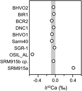Fig. 11 Ca mass-dependent isotope data for various standards representatively shown as δ⁴²Ca. The grey bar is the 2 sd based on the igneous rock standards. Internal errors are smaller than symbols.

Resolvable mass-dependent differences from SRM 915b were only found for the seawater standard OSIL AL (δ⁴²Ca = −0.53 ± 0.02) and SRM 915a (δ⁴²Ca = +0.42 ± 0.02). Both of these results are in agreement with data reported elsewhere^5,13,23 that were obtained by double-spike TIMS techniques. The excellent agreement between our data and earlier results measured using a different technique suggests that the MC-ICPMS approach described here using the standard-sample bracketing method is also well-suited to the precise and accurate determination of mass-dependent Ca isotope fractionation.

The mass-independent Ca isotope composition of the igneous rock standards as well as that of seawater presented here is identical to SRM 915b, whether measured precisely by TIMS (⁴⁰Ca), or by MC-ICPMS (⁴³Ca, ⁴⁶Ca, ⁴⁸Ca) (Table 4). Previously published mass-independent Ca isotope compositions of terrestrial reservoirs are scarce, and have been mostly focused on the study of potential variations in the ^40/44Ca ratio.^7–10 For example, Caro et al.¹⁰ recently reported highly-precise μ⁴⁰Ca data for various geological materials, but they did not present their μ⁴³Ca data. Although our results are in broad agreement with those reported by Caro et al.¹⁰ for mantle-derived rock samples and seawater (considering the external reproducibility of 80 ppm for our μ⁴⁰Ca data), we note an apparent negative offset of ∼70 ppm in our data compared to that of ref. 10, which may not be present in the μ⁴³Ca data. This offset could, in principle, reflect a difference in the ^40/44Ca ratio of the reference standards, given that our data are reported relative to SRM 915b whereas ref. 10 used SRM 915a as a reference standard. Although our analysis of an aliquot of the SRM 915a did not show a resolvable difference in the absolute ^40/44Ca ratio of the two standards (Table 4), the ^40/44Ca ratio for SRM 915a measured here (47.1662 ± 0.0023) is higher by ∼85 ppm compared to that reported by Caro et al.¹⁰ Because this offset is not apparent when comparing the absolute ^40/44Ca ratio of the seawater samples analyzed by Caro et al.¹⁰ and us, we suggest that the ⁴⁰Ca composition of the SRM 915a standard may be heterogenous.

Although comparison with previously published data for the heavy Ca isotopes is difficult considering that the most precise TIMS data reported so far^7,8 has an external reproducibility that is more than an order of magnitude less precise than the data reported here, our data provides a few interesting observations. As we do not expect mass-independent isotope variability on Earth, the data presented here for two fractionated samples (SRM 915a and OSIL AL) allows us to investigate the type of mass fractionation these two samples experienced. This is because all mass fractionation in the sample is assumed to be kinetic and corrected for by the kinetic mass fractionation law. Therefore, if a sample experienced mass fractionation that was non-kinetic by nature, the kinetic mass fractionation law applied here should create an artificial anomaly that is related to the size of the mass-dependent mass fractionation between the sample and standard and the original kind of mass fractionation that produced the difference in mass-dependent isotope composition. The only sample that shows such a resolvable effect is SRM 915a (μ⁴³Ca = +62.7 ± 6.1; Table 3), which can best be explained by equilibrium fractionation effects (see discussion below).

3.5.3 Implications for Ca isotope fractionation in the carbonate cycle. The calcium isotope composition of seawater is a result of isotope fractionation during marine carbonate formation by organic and inorganic processes, as well as from riverine influx.⁴ There has been some debate as to whether Ca isotope fractionation during carbonate precipitation in nature occurs as a kinetic³⁰ or as a equilibrium³¹ process. It can be calculated that Ca isotope fractionation that is the result of pure equilibrium fractionation would create a μ⁴⁸Ca = −12 ppm anomaly per +0.1‰ difference in δ⁴²Ca between standard and sample when mass fractionation is corrected for using the kinetic law. For seawater with a δ⁴²Ca of −0.53‰ this would result in a μ⁴⁸Ca of +64 ppm relative to BSE. However, there is no observable difference in μ⁴⁸Ca between seawater and BSE at the external reproducibility of our technique (±12.5 ppm). This suggests that the dominant mechanism of mass-dependent isotope fractionation between BSE and seawater must follow a kinetic law, which is in agreement with previous suggestions.³⁰

3.5.4 Composition of SRM 915a. SRM 915a has a mass-dependent isotopic composition that is significantly different from BSE (Table 3 and 4). The isotopic composition of SRM 915a relative to SRM 915b has been established to be δ^44/40Ca = −0.72 ± 0.05‰,^13,23 which is in agreement with the data presented here (δ^42/44Ca = +0.42 ± 0.02). The mass-independent composition of SRM 915a relative to SRM 915b differs from those of the rock standards. Explicitly, when SRM 915a is measured by MC-ICPMS and corrected for mass fractionation by the kinetic law, its μ⁴⁸Ca_MC-ICPMS is offset from SRM 915b by +62.7 ± 6.1 ppm (Table 3). However, when the MC-ICPMS data are corrected using the equilibrium instead of the kinetic law, the μ⁴⁸Ca_MC-ICPMS anomaly is reduced to +12.7 ± 5.2 ppm. This significant reduction of the anomaly to a value that is within error of zero suggest that the mass-dependent isotope fractionation relative to Earth experienced by SRM 915a contains a significant component of equilibrium fractionation. Further, the observed small differences in the mass-dependent Ca isotopic composition (⁴⁰Ca/⁴⁴Ca; Table 4) of our data and that of Simon et al.⁸ and Caro et al.¹⁰ suggests that there might be a potential isotope heterogeneity in the NIST SRM 915a standard that seems at least to be detectable in μ⁴⁰Ca.

Because of the resolvable differences in the mass-dependent as well as mass-independent composition of SRM 915a and the observations of much smaller or nonexistent differences between BSE and SRM 915b, we suggest to use SRM 915b as standard for future studies of the mass-dependent as well as mass-independent Ca composition of rock samples.

4 Conclusions

The conclusions of this study can be summarized as follows:

1. A new approach for high-precision Ca measurements using both Neptune Plus (MC-ICPMS) or Triton (TIMS) for sequential isotopic analysis has been described. The technique allows to cover the full mass range from ⁴⁰Ca to ⁴⁸Ca with the best possible precision for each isotope. Estimated external reproducibilities are 80 and 23 ppm for μ⁴⁰Ca_TIMS and μ⁴³Ca_TIMS and 1.8, 45 and 12.5 ppm for μ⁴³Ca_MC-ICPMS, μ⁴⁶Ca_MC-ICPMS, and μ⁴⁸Ca_MC-ICPMS. This represents a more than 45-, 120-, and 18-fold improvement over the most precise μ⁴³Ca, μ⁴⁶Ca, and μ⁴⁸Ca data presented so far.

2. Our mass-dependent isotope data demonstrates that comparable precision can be achieved by MC-ICPMS to the more traditional double-spike TIMS technique while also obtaining information on the mass-independent composition.

3. The mass-independent data presented here suggest that the Ca mass-dependent isotope fractionation of modern seawater predominantly results from kinetic precesses. This implies that the biogenic and inorganic processes of carbonate formation fractionate Ca kinetically from seawater.

4. Precise measurements of SRM 915a indicate that the mass-dependent Ca isotopic composition of this carbonate standard is not only significantly different from BSE (δ^42/44Ca = +0.42 ± 0.02), but also contains a component that cannot be explained by purely kinetic fractionation. Moreover, comparison of our μ⁴⁰Ca data with that of Caro et al.¹⁰ suggests that the SRM 915a standard may be heterogenous, at least in its ⁴⁰Ca composition. These observations indicate that the SRM 915b, which has a Ca mass-dependent and mass-independent isotope composition that is identical to the BSE, is a better reference material to study the Ca isotope composition of terrestrial and non-terrestrial materials.

Acknowledgements

Financial support for this project was provided by the Danish National Research Foundation, the Danish Natural Science Research Council, and the University of Copenhagens Programme of Excellence. The Centre for Star and Planet Formation is funded by the Danish National Research Foundation and the University of Copenhagens Programme of Excellence. We would like to thank A. Eisenhauer for providing a sample of SRM 915a. We are grateful for the helpful comments provided by two anonymous reviewers.

References

1. B. Meyer, Phys. Rep., 1993, 227, 257–267.
2. W. Russell, D. Papanastassiou and T. A. Tombrello, Geochim. Cosmochim. Acta, 1978, 42, 1075–1090.
3. A. Heuser, A. Eisenhauer, N. Gussone, B. Bock, B. Hansen and T. Nagler, Int. J. Mass Spectrom., 2002, 220, 385–397.
4. D. DePaolo, Rev. Mineral. Geochem., 2004, 55, 255–288.
5. M. Amini, A. Eisenhauer, F. Bohm, C. Holmden, K. Kreissig, F. Hauff and K. Jochum, Geostand. Geoanal. Res., 2009, 33, 231–247.
6. J. I. Simon and D. J. Depaolo, Earth Planet. Sci. Lett., 2009, 289, 457–466.
7. F. Moynier, J. I. Simon, F. A. Podosek, B. S. Meyer, J. Brannon and D. J. Depaolo, Astrophys. J., 2010, 718, L7–L13.
8. J. I. Simon, D. J. Depaolo and F. Moynier, Astrophys. J., 2009, 702, 707.
9. K. Kreissig and T. Elliott, Geochim. Cosmochim. Acta, 2005, 69, 165–176.
10. G. Caro, D. A. Papanastassiou and G. J. Wasserburg, Earth Planet. Sci. Lett., 2010, 296, 124–132.
11. E. T. Tipper, J. Gaillardet, A. Galy, P. Louvat, M. J. Bickle and F. Capmas, Global Biogeochem. Cycles, 2010, 24, GB3019.
12. C. Bouman, M. Deerberg and J. B. Schwieters, NEPTUNE and NEPTUNE Plus: Breakthrough in Sensitivity using a Large Interface Pump and New Sample Cone, Thermo Fisher scientific, Bremen, Germany technical report, 2009.
13. F. Wombacher, A. Eisenhauer, A. Heuser and S. Weyer, J. Anal. At. Spectrom., 2009, 24, 627–636.
14. E. T. Tipper, P. Louvat, F. Capmas, A. Galy and J. Gaillardet, Chem. Geol., 2008, 257, 65–75.
15. W. Russell and D. Papanastassiou, Anal. Chem., 1978, 50, 1151–1154.
16. A. Galy, N. Belshaw, L. Halicz and R. O'Nions, Int. J. Mass Spectrom., 2001, 208, 89–98.
17. M. Schiller, J. A. Baker and M. Bizzarro, Geochim. Cosmochim. Acta, 2010, 74, 4844–4864.
18. E. Horwitz, D. McAlister, A. Bond and R. Barrans, Solvent Extr. Ion Exch., 2005, 23, 319–344.
19. A. Pourmand and N. Dauphas, Talanta, 2010, 81, 741–753.
20. M. W. Wilding and D. W. Rhodes, J. Chem. Eng. Data, 1970, 15, 297–298.
21. C. Paton, J. Hellstrom, B. Paul, J. D. Woodhead and J. Hergt, J. Anal. At. Spectrom., 2011 10.1039/C1JA10172B.
22. M. Bizzarro, C. Paton, K. Larsen, M. Schiller, A. Trinquier and D. Ulfbeck, J. Anal. At. Spectrom., 2011, 26, 565–577.
23. A. Heuser and A. Eisenhauer, Geostand. Geoanal. Res., 2008, 32, 311–315.
24. F. Wombacher and M. Rehkämper, J. Anal. At. Spectrom., 2003, 18, 1371.
25. D. Wielandt and M. Bizzarro, J. Anal. At. Spectrom., 2011, 26, 366.
26. K. Newman, P. A. Freedman, J. Williams, N. S. Belshaw and A. N. Halliday, J. Anal. At. Spectrom., 2009, 24, 742–751.
27. L. Halicz, A. Galy, N. Belshaw and R. O'Nions, J. Anal. At. Spectrom., 1999, 14, 1835–1838.
28. S. Hart and A. Zindler, Int. J. Mass Spectrom. Ion Processes, 1989, 89, 287–301.
29. R. Andreasen and M. Sharma, Science, 2006, 314, 806–809.
30. N. Gussone, A. Eisenhauer, A. Heuser, M. Dietzel, B. Bock, F. Bohm, H. J. Spero, D. W. Lea, J. Bijma and T. F. Nagler, Geochim. Cosmochim. Acta, 2003, 67, 1375–1382.
31. C. S. Marriott, G. M. Henderson, N. S. Belshaw and A. W. Tudhope, Earth Planet. Sci. Lett., 2004, 222, 615–624.

---