Studying Smad2 intranuclear diffusion dynamics by mathematical modelling of FRAP experiments

Abstract

We combine Fluorescence Recovery After Photobleaching (FRAP) experiments with mathematical modelling to study the dynamics inside the nucleus of both the TGF-β-sensitive transcriptional regulator Smad2, and Green-Fluorescent Protein (GFP). We show how combining modelling with bleaching strips of different areas allows a rigorous test of whether or not a protein is moving via diffusion as a single species. As noted recently by others, it is important to consider diffusion during the bleaching process. Neglecting it can cause serious error. Also, it is possible to use the bleaching process itself to provide an extra consistency test to the models predicting the recovery. With our method we show that the dynamics of GFP are consistent with it diffusing as a single species in a uniform environment in which flow is negligible. In contrast, the dynamics of the intracellular signal transducer Smad2 are never consistent with it moving as a single species via simple diffusion in a homogeneous environment without flow. Adding TGF-β slows down the dynamics of Smad2 but even without TGF-β, the Smad2 dynamics are influenced by one or more of: association, flow, and inhomogeneity in space of the dynamics. We suggest that the dynamics inside cells of many proteins may be poorly described by simple diffusion of a single species, and that our methodology provides a general and powerful way to test this hypothesis.

---

1. Introduction

Most protein molecules are in constant motion inside a cell, and many need to move across the cell to perform their function. For example, a protein that is part of a signalling pathway may need to find a binding partner and the site on the DNA where it controls transcription. We need to know how proteins move inside cells, both to understand how they function in cells and because changes in mobility provide evidence of changes in protein state, e.g., a slow down suggests that the protein is binding to something. Typically, many proteins not anchored to membranes or other cellular structures are assumed to move via diffusion in the cytoplasm and the nucleus, and are often referred to as “freely diffusible”. Here, we show how to combine Fluorescence Recovery After Photobleaching (FRAP) experiments with modelling to test whether or not a protein's mobility is really diffusive. We find that the cell-signalling protein we study, Smad2, appears never to exist as a single freely diffusing species, suggesting that its dynamics are more complex than previously thought. We believe that understanding cell signalling will require a quantitative understanding of protein dynamics and that our methodology can contribute to this understanding.

FRAP is perhaps the most widely applied experimental technique for studying protein dynamics in vivo.^1–3 Typically, a fluorescent protein such as Green Fluorescent Protein (GFP) is fused to a protein of interest and the resulting fusion protein is expressed in cells. Using a laser scanning microscope, a region of the cell is then bleached. For example, in pioneering studies by Axelrod and co-workers,^4–6 a small region with a size set by the width of the laser beam was bleached. If the dynamics of the protein are diffusive, the diffusion constant D of the protein may be estimated from D ≃ w²/τ. Here w is the width of the beam, and τ is the time for the fluorescence to recover in the bleached region.

However, there are a number of reasons why the dynamics of a protein may not be well described by the solution of the diffusion equation for a single component in a uniform environment. Perhaps the most obvious are:

1. The dynamics and hence the fluorescence recovery can be governed by binding reactions, e.g., to a large static structure. In that case the recovery rate depends on the off-rate of the binding reaction.

2. Recovery can be caused by flow, in which case the recovery time measures the flow rate rather than D.

3. The protein may exist as more than one species with the different species having differing mobility, e.g., as a monomer and a more slowly diffusing dimer, where the dimer formation and breakdown occurs on timescales longer than that of the FRAP experiment.

4. The cell compartment may be inhomogeneous, i.e., consist of regions where the mobility of the protein is high and regions where it is low.

If any of these are true, the dynamics will be more complex than simple diffusion and will be characterised by a number of parameters rather than just a single diffusion constant. In this case, the FRAP curve may not provide enough information to reliably determine all the parameters.⁷ To test whether recovery is due just to simple diffusion, we use the flexibility offered by modern laser-scanning confocal microscopes to bleach areas of different sizes within a cell nucleus. Diffusion has the well known property that the characteristic timescale scales as the length squared. Thus, in the case of diffusion-limited dynamics, the recovery time will depend on the width of the bleaching area,^8,9 but will be independent in the case of dynamics that are, for instance, reaction-limited.

In contrast to earlier studies, we use relatively large bleaching areas. This approach has the advantage of significantly reducing experimental noise and results in slower, and hence easier to measure, fluorescence recovery. Both these effects allow more accurate, more quantitative, experiments. It is also important to notice that when bleaching large areas, we average over any heterogeneities in mobility over smaller lengthscales. The fluorescence recovery curves present us with information of the average properties of the region sampled. The nuclear compartment is known to be heterogeneous, e.g., due to nucleoli, and so we observe an average mobility in and outside of nucleoli. Simply speaking, if regions exclude the protein, then protein has to diffuse around the region. This is known to reduce the effective diffusion constant on lengthscales larger than the excluding regions, but only by relatively small amounts. See for example the work of Hrabe et al.¹⁰ and Ölevsky et al.¹¹ Also, if a region contains a high concentration of binding sites then locally the fluorescence recovery may be dominated by the unbinding rate from these sites.¹² This will only show up in FRAP experiments with large bleaching areas if the number of sites is large enough and the unbinding rate is slow in comparison to recovery by motion across this area.

Since bleaching can take a significant amount of time especially if we wish to bleach large areas, we explicitly model diffusion during the bleaching step, and demonstrate that this can provide additional information on the protein dynamics. Although most previous work has not considered diffusion during bleaching, there are some studies which do. Yang et al.¹³ have shown how a simple correction can account for diffusion during bleaching in their systems of a protein in a glycerol solution and a protein on the surface of a human B cell line. Vinnakota et al.¹⁴ also modelled diffusion during bleaching. Like Yang et al. they did this for a membrane-associated protein, and like Yang et al. found that diffusion was significant during bleaching, despite the rather slow diffusion of a protein associated with a membrane. Castle and Odde¹⁵ have recently found that diffusion during bleaching can also be important in FRAP experiments performed on the larger length scales in Drosophila embryos.

1.1 The intracellular signal transducer Smad2

Here, we combine FRAP experiments and mathematical modelling to study the mobility in the nucleus of Smad2, which transmits signals from TGF-β-type growth factors from the membrane into the nucleus. For an introduction to the mechanism of TGF-β/Smad signalling, see the reviews of Shi and Massagué,¹⁶ and Schmierer and Hill.¹⁷ Briefly, TGF-β binds to the extracellular domain of transmembrane serine-threonine kinase receptors, and leads to the induction of their kinase activity. Once active, these kinases phosphorylate Smad2 at its extreme C-terminus. This phosphorylation triggers complex formation between phospho-Smad2 and Smad4. These complexes accumulate in the nucleus, where they bind to DNA and, through interaction with transcription factors and chromatin modifiers, regulate target gene expression.¹⁸ Unlike other Smads, Smad2 cannot bind to DNA on its own due to a short amino acid insertion in its MH1 domain (the MH1 domain is a functional DNA-binding domain in other Smads but not in Smad2). Thus, Smad2 requires the DNA-binding activity of Smad4 to target the phospho-Smad2/Smad4 complex to suitable binding sites in target gene promoters.

In uninduced cells, very little Smad2 is found in the nucleus, see Fig. 1, and FRAP experiments¹⁹ have shown that Smad2 is very mobile within the nuclear compartment under these conditions. However, in cells treated with the growth factor TGF-β, the nuclear mobility of Smad2 is strongly decreased. This decrease in mobility is presumably due to Smad2 forming a complex with Smad4 and this complex binding to DNA/chromatin, but there may be other, as yet uncharacterised binding interactions. Motivated by the results of earlier work,^19–21 we proposed the following two hypotheses:

Fig. 1 (A) Confocal microscopy images of the nuclei of a HaCaT cell line stably expressing a Smad2-GFP fusion. The top and bottom rows are for uninduced and induced cells, respectively. Note that in uninduced cells the nucleus is darker than the surrounding cytoplasm while in induced cells the nucleus is brighter. This is due to the low nuclear concentration of Smad2-GFP in uninduced cells and its much higher nuclear concentration in TGF-β induced cells. The scale bar is 10 μm. (B) Simulation image of the cell nucleus immediately after the bleach, for a circular nucleus. The nuclear diameter is 17 μm, the width of the bleaching region is W = 2.9 μm, D = 2.5 μm²s⁻¹ and the fraction of the available protein bleached in every scan, P₀, is 0.076. (C) Cross section of the bleached profile in (B). The black circles are the numerical data and the red curve is a Gaussian fit to this data. (D) Schematic of the bleaching process. The bleached region is composed of n lines, one pixel wide and of length L. Note that the laser sweeps the whole length of the field of vision, but the power is modulated to only bleach the region of interest. After sweeping one line, the laser sweeps the next line in the opposite direction. When finished with all the lines, the laser returns to the starting point to begin a new scan.

1. In the absence of TGF-β induction, the nuclear mobility of Smad2 is purely diffusive and is not substantially affected by associative reactions.

2. TGF-β-induced complex formation with Smad4 gives rise to two species, monomeric Smad2 and complexed Smad2.²¹ While the monomeric Smad2 behaviour remains diffusive, the complex has associative reactions. In this case, in cells exposed to TGF-β the dynamics of the total Smad2 concentration is no longer simple diffusion.

In this work we test these hypotheses by combining FRAP experiments with mathematical modelling.

1.2 Confocal microscopy and cell lines

Microscopy was performed using a Zeiss LSM 510 confocal microscope. Imaging was performed with a Plan Apochromat 63x 1.4 NA oil immersion objective using 488 nm excitation and collecting emission using a 500–550 nm bandpass filter. All live cell imaging was performed at 37 °C. The HaCaT keratinocyte cell lines expressing GFP-tagged Smad2 or photoactivatable GFP have been described and characterised in detail previously.¹⁹ The cells express GFP-Smad2 at approximately endogenous levels and show no signs of basal or autocrineTGF-β signalling.¹⁹ Photoactivatable GFP was photoactivated prior to the bleaching experiments using a blue diode laser at 405 nm.

Our FRAP protocol and data normalization are as follows. Ten pre-bleach pictures were taken, then a rectangular bleach area which is the complete width of the nucleus along the y direction and of width W along the x direction was scanned a number of times with 100% laser power. The total bleaching time was 500 ms (780 ms for GFP). See Fig. 1(D) for the path traced out by the bleaching laser beam, and Fig. 1(A) for images of cells during the FRAP experiments. Note that the bleached stripe is always approximately in the middle of the nucleus along the x axis. Directly after the bleach, up to 300 images were taken at a frequency of 5 Hz and a size of 256 × 256 pixels. The laser intensity was such that photobleaching was negligible during image acquisition in all experiments. For normalization, fluorescence of the bleach region and of the entire compartment were both corrected for background fluorescence and normalised to the average pre-bleach fluorescence in the corresponding region. Further normalization was performed by dividing the background-corrected single-normalised fluorescence of the bleach region by the background-corrected single normalised fluorescence of the entire compartment. Data from 10 cells (20 for unfused GFP) were pooled into an average recovery curve, which was then further normalised such that the initial fluorescence after the bleach was zero and full recovery was 1. In control experiments FRAP-curves were recorded over longer time periods and full recovery was observed in all cases, excluding the presence of an immobile nuclear fraction of Smad2. Our average curves are created by pooling 10 curves from different nuclei. The bleaching areas in the different nuclei contained varying fractions of dark regions (nucleoli). No statistically significant differences were observed between these curves.

For cells without TGF-β, stripes of width W = 2.9 μm or 1.16 μm were bleached across the centre of the cell nucleus. TGF-β was used at a concentration of 2 ng ml⁻¹, and for TGF-β-treated cells, the bleached stripes had widths of 2.9 or 0.58 μm. The total bleaching time of 500 ms was kept constant for all the cells expressing GFP fused Smad2. This corresponds to 54 scans across the complete bleaching area in the case of the 2.9 μm wide area, 135 scans for 1.16 μm and 270 scans for 0.58 μm. Each scan is of the complete area we wish to bleach and is composed of a number of sweeps by the laser beam across the full width of the nucleus, approximately 15–20 μm. Thus what we call a sweep is just one movement of the laser beam from left to right, and a scan is composed of however many sweeps are required to bleach a region of the desired width. The width of the beam is taken to be the pixel size, 2w = 0.29 μm. Thus the bleaching area of width 0.58 μm was 2 pixels across and so a scan here was of two sweeps, etc. The beam sweeps across an average nucleus every δt = 0.93 ms. As a control, the dynamics of unfused GFP was studied by bleaching a strip of 2.9 μm for a total time of 780 ms which corresponds to 85 scans of the bleached area.

2. Modelling FRAP data for diffusing proteins

Here, we model a FRAP experiment in two stages which we treat independently, the bleaching stage and the recovery stage. The bleaching stage is modelled as a given number of scans of the bleaching region by the laser. Each scan is assumed to be sufficiently fast to be considered instantaneous however bleaching consists of many scans and we do consider diffusion between one scan and the next. We found that assuming that bleaching occurs instantaneously leads to significant error. Indeed, the fractions bleached both within the bleaching area and within the compartment depend on the diffusion constant, and so we are able to obtain estimates of the diffusion constant from these fractions.

The recovery stage is modelled by calculating the time and space evolution of the profile resulting from the bleaching stage. The resulting recovery curve can then be fit to the experimental recovery curve. In our experiments, stripes of different widths are bleached. These stripes cover the whole length of the cell nucleus. Also, the numerical aperture was such that the complete height of the nucleus is bleached, effectively reducing our problem to one dimension.

We start by assuming that the tagged protein exists as one species that moves via simple diffusion. Then the evolution of the protein concentration, A, is given by

where D is the diffusion constant of the protein and ∇² is the Laplacian operator.

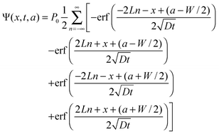
First, we model the nucleus as a square box of side L with zero flux boundary conditions, i.e., we assume that protein transport into and out of the nucleus is negligible on the timescale of the FRAP experiment.¹⁹ In addition, we check that modelling what is an oval nucleus by a square is an innocuous approximation by numerical modelling of a circular nucleus. Bleaching is done across the complete width of the nucleus and the bleaching lines are taken as parallel to the y axis, see Fig. 1(D). The profile is one dimensional, A(x,t), and, using Green's functions,²² can be written as

where G(x,t) is the appropriate Green's function for the problem, x_i is the position of the ith boundary, z_i the boundary conditions at the ith boundary, and F(q) is the spatial distribution at time t = 0.

Following Beck et al.²² we can calculate the Green's functions for our geometry, which is a one-dimensional box with zero-flux boundary conditions at x = 0 and x = L. First, we show the Green's function calculated as an expansion in eigenfunctions of the Laplacian operator that satisfy our boundary conditions:

Where q and τ are the projection coordinates that we have to integrate over to propagate the solution in time and space. Now, the Green's function for the prescribed geometry and boundary conditions using the method of images is: From the factors involving time in both functions we can see that the first expression has a better convergence for longer times, while the second one is more suitable for smaller time intervals. With these expressions in hand, we can proceed to model both stages of the experiment.

2.1 The bleaching stage

Within our square-nucleus model, we can describe the concentration A(x,t) at point x and time t of the bleachedprotein by the reaction-diffusion equationWhere D is the diffusion constant and K is the space and time dependent bleaching rate. The point spread function and path followed by the laser are encoded in K, which as a result is a complex function of time and space. With this K, eqn (5) is very complicated and so impossible to solve analytically. However, it can be solved numerically,^14,23 or a simple correction term for diffusion during bleaching can be used.¹³ In this work, we take advantage of the linearity of the diffusion equation and model the bleaching process as the superposition of multiple instantaneous individual bleaches.

In our model, the bleach process consists of N scans of the complete width of the nucleus along the y-axis and of length W along the x-axis. This region is in the centre of the nucleus, i.e., from x = L/2 − W/2 to x = L/2 + W/2. Each scan of the bleaching region consists of n = W/(2w) line sweeps of the laser beam, where 2w is the 1/e² width of the laser beam (=one pixel). Scanning of the region is performed line by line moving in a zigzag pattern as shown in Fig. 2. Thus there are three timescales: (1) the time for a single sweep across the width of the nucleus, δt = 0.93 ms, (2) the time for a complete scan of the bleaching region, Δt = nδt, and (3) the bleaching time nNδt.

Fig. 2 (A) Comparison between the profiles obtained from an instantaneous bleach of the entire bleaching region, and a bleach of n line sweeps. In both panels, the black curve is the resulting bleached profile after n = 10 line sweeps (from left to right) of the Gaussian point spread function at δt = 0.93 ms intervals. Each line sweep is of width w = 0.29 μm. In the left panel, each individual sweep is shown (in different colours). The spread of the older (on the left) lines is readily visible. In the right panel, the red curve is at a time Δt = 9.3 ms after an instantaneous bleach of the entire bleaching region of width W = 2.9 μm with a step function profile. The nucleus is square with sides of length 17 μm. The bleaching depth P₀ = 0.04 and we take a typical value for D of D = 5.25 μm²s⁻¹. (B) The half-life of fluorescence recovery in the bleached region is plotted as a function of D. The black curve is the result of numerical calculations, and the red curve is a fit to this data of a function of the form t_1/2 = c/D. The half-life is defined by normalizing the fluorescence so that the initial fluorescence in the region is 0, the final is 1 and then the half recovery time is the time when the fluorescence is 0.5. The calculations are for a circular nucleus of diameter 17 μm. The bleaching strip across the centre of the nucleus is W = 2.9 μm wide. The bleaching parameter is kept fixed at P₀ = 0.02, and we use the typical value for D of D = 5.0 μm²s⁻¹.

In our system, the bleaching time of 500 or 780 ms is two orders of magnitude larger than the sweep time. The sweep time is so short that diffusion cannot keep up with the scanning beam, which crosses a nucleus in less than 1 ms. Indeed, as the largest width we bleach (2.9 μm) is only 10 line sweeps, a scan takes at most 10 times longer, i.e. less than 10 ms. Even assuming a very large diffusion constant of 100 μm²s⁻¹ a protein will only diffuse a micrometre in that time. However, in the bleaching time which is of order 1 s, even if D is only 10 μm²s⁻¹, it will diffuse several micrometres, which is comparable to the width of the bleached area. Thus, as we will see, we can neglect diffusion over the timescale of a scan, Δt < 10 ms, but not over the total bleaching time.

2.1.1 Diffusion during a scan can be neglected. Here, we will explicitly calculate diffusion during a scan, and consider the effect of the point spread function (psf) of the laser beam, in order to show that both can be neglected. Having done so we will treat each scan as being instantaneous, and each bleach as being a top-hat function, when we fit to the experimental data for bleaching.

We calculate the resulting profile after a single scan as follows. We can split a single scan into the individual contributions of each line sweep. Each line sweep is modelled as instantaneous and separated by a time interval δt. Now, we need to know how much of the previously bleached protein will diffuse into the region that is going to be bleached next. This is accomplished by solving the diffusion equation for an individual sweep, approximating the psf of the laser with a Gaussian function,

Here Ω(x,t,x₀) is the resulting profile after time t when the point spread function Ω(x,0,x₀) centred in x₀ is bleached at t = 0. Using the Green's function in the previous section, eqn (3), we calculate the solution asNow, if we take into account diffusion from a previously swept line to the next ones, we can approximate the resulting distribution after sweeping all the lines once, S(x,Δt), as:Here P₀ is the bleach depth. The coefficient Γ_j is the average of the remaining unbleached protein over the width of the jth line (the line being bleached), so effectively, we are bleaching our point spread function every time with an amplitude proportional to the protein left. Now, the amount of protein bleached at every step depends on previous steps. We can calculate sequentially the coefficients Γj aswhere the brackets indicate that the average is taken over the width of the jth line.

Using eqn (8), we have calculated the resulting profile after one scan of the bleaching area (of 10 line sweeps) which is shown in Fig. 2(A). In the right panel of Fig. 2(A), we can see that the resulting profile (black curve) is well approximated by the profile obtained by bleaching a step function covering the whole width of the bleach area (red curve). This is after only one scan, the difference after many scans will be smaller. Thus, diffusion during a scan can be neglected and from now on we will do so.

2.1.2 Modelling bleaching as a series of instantaneous scans of the bleaching region. To obtain bleached fractions to compare to experiment, we model bleaching as a series of N instantaneous scans of the bleaching region. The bleaching function for a scan is taken to be a step function of depth P₀. So the fraction of protein bleached at point x isFor a bleaching region centred at a. Here we will only use a = L/2.

We calculate the distribution of the fraction of protein after bleaching using the Green's function method described above. Then the distribution of the fraction of protein bleached at time t after the profile F is bleached at time t = 0, is given by

This gives the fluorescence distribution after one scan. In the right-hand panel of Fig. 2(A) we have plotted the fraction bleached a time Δt after an assumed instantaneous scan of 10 lines wide (red curve), and compared it with the fraction bleached after 10 individual instantaneous line bleaches, each taking δt = Δt/10 s (black curve). Note that the two curves are very similar except on the right of the bleaching region where the last line sweep occurred. After multiple scans, the difference between the curves with instantaneous sweep bleaches and instantaneous scan bleaches becomes very small—much smaller than in Fig. 2(A). Thus for the diffusion constants we consider, our approximation of taking scans to be instantaneous introduces very little error.

We can now proceed to calculate the final distribution of the fraction of protein bleached after N scans, H(x,N). In the first scan, the fraction bleached is just F(x,L/2). However, in the second scan the bleaching is reduced due to the fact that we have less protein in the bleaching region due to the first scan. Also, there will be diffusion of the protein between the first and the second scans, which we must take into account. For the third scan we need to account for the bleaching in the first two scans plus diffusion, and so on.

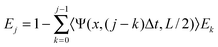
To calculate the profile bleached after N scans we define the average of the fraction remaining in the bleached region after j bleaches as E_j, which is given for j ≥ 1 by

where the average 〈〉 is taken over the bleaching region from L/2 − W/2 to L/2 + W/2. Also, E₀ = 1.

Again, using the fact that the equations are linear we can simply sum the contributions to the final bleached fraction as a function of position H(x,N), taking into account the diffusion that takes place between each scan and the end of the bleaching stage,

2.1.3 Numerical modelling of a circular nucleus. As discussed in the previous section, approximations were made to obtain the formulas presented. In particular we assumed each scan was instantaneous, and we also assumed the nucleus was square, when it is closer to oval, see Fig. 1. Numerical simulation allows us to simulate more accurately the bleaching process, and so to check our assumptions. We can do this by specifically bleaching line by line in the same way the laser does in the actual experiment. Given these conditions, the diffusion equation was solved in a circle of the same size as the cell nucleus using the finite-difference method on a two dimensional 100 × 100 site lattice. We obtained the pair of parameters (D and P₀) that best fit the experimental measures of total amount of fluorescence lost and average fluorescence in the bleached region at time zero of the recovery stage. To calculate the error, we calculated the biggest deviation in the parameters that would still predict values inside one standard deviation of the mean of the experimental data.

2.2 The recovery curves

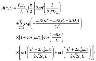
We model the profile of the bleached fraction at the end of the bleaching process as a Gaussian: B₀exp[−(x − x₀)²/(2c²₀)]. This is a very good approximation to the true distribution, see Fig. 1(C). This function has two parameters, maximum bleaching depth, B₀, and width, c₀. The experiments yield two numbers: the average fraction of protein bleached in the complete nucleus, E_n, and the average fraction of protein bleached in the bleaching region of width W, E_W. These are related to our Gaussian profile viaThus, we take the values of E_n and E_W from experiment and fit B₀ and c₀ to them. This gives us our bleaching profile at the start of the recovery.

If we set this as time t = 0 for the recovery stage, then again using a Green's function method the protein concentration as a function of position x at time t > 0 is given by

The average reduction in fluorescence at time t in the bleaching region isThe standard FRAP curve is a plot of the average fluorescence in the bleached region as a function of time, normalised so that it tends to one at long times, and is zero at time t = 0.

As the fraction bleached in the bleaching region starts at E_W and ends as E_n the normalised fluorescence in the bleached region is given by

Finally, we note that it is essential to take the finite size of the nucleus into account. For the larger values of D we consider, the FRAP timescale is comparable to the timescale for diffusion across the complete nucleus. This is illustrated in Fig. 2(B), where we have plotted the half-life for fluorescence recovery as a function of D. For a bleaching region of fixed size, the half-life for FRAP in an infinite volume should simply scale as 1/D as that provides the only relevant timescale. However, in Fig. 2(B) we see large deviations from this simple scaling, due to the finite size of the nucleus.

2.3 Comparison with earlier modelling work

Here, we have focused on modelling the details of the FRAP experiments, including the bleaching stage. We have shown how to model analytically and extract information from the bleaching stage. This is not only useful as a check for diffusive behaviour, because bleaching occurs on shorter timescales than recovery, it allows us to obtain information on protein mobility on those shorter timescales. Diffusion during bleaching also needs to be taken into account when modelling FRAP of larger regions.

In earlier work diffusion during bleaching has been studied both via numerical simulations of the whole recovery experiment,¹⁴ analytically by correcting the half recovery time to take into account the spread of the bleached profile¹³ and following semi-analytically the bleaching process and the spreading of the bleaching profile.²⁴ Taking into account diffusion during bleaching allow us to bleach larger regions and model the behaviour correctly. Bleaching larger regions is also useful as it reduces the noise to signal ratio, thus allowing more accurate studies. These advantages thus apply to the work here as well as that of Yang et al.¹³ and Vinnakota et al.¹⁴ Yang et al.'s simple correction is useful if a simple correction for diffusion during bleaching is required, whereas Vinnakota et al.'s methodology allows simultaneous fitting of the bleaching and recovery stages. Here we will fit to bleaching and recovery separate in order to obtain two values for D, which acts as a consistency check. We have only considered diffusion, not reaction and diffusion.

Earlier work on diffusion has derived useful analytical results for the bleaching of some geometries such as disks and rectangles,^25,26 and also done the calculations numerically.²⁷ However, many proteins of interest are believed to bind to other proteins—which may either be diffusing themselves or be part of larger structures. To model these proteins, reaction-diffusion models are used. There has been work that has considered species that both react and diffuse. See for example the work of Sprague et al.,^9,28,29 and of others^7,30 And for multiple species binding and diffusing.³¹ However, Zadeh et al.⁷ showed that it is not possible to determine simultaneously the diffusion constant and the two reaction parameters (on and off rate constants) from a single recovery curve.

Some earlier work used inverse Laplace transforms, which can be computationally demanding, especially when fitting. An alternative is to model the diffusion out of the bleached region as interchange between two compartments, simplifying the analytical solution.¹ This approach has been shown to be equivalent to the solving the full reaction-diffusion equations.³² It is always possible to solve the diffusion equation numerically. This approach is flexible but generally requires more computational time.^33,34

In addition to simple one-component reaction-diffusion models, other models have been tried. For example, models with two or more reacting and diffusing components,^35,36 models with a continuous distributions of diffusion constants,³⁷ and models with an interchange between free monomers and immobile polymerised filaments.³⁸ Whichever model we choose, FRAP experiments can be used to monitor the change in the dynamics in response to a change such as that provided by an external stimulus^39,40

3. Results

To test if the fluorescence recovery is dominated by diffusion, we bleached stripes of different widths as suggested by Gribbon and Hardighan,⁸ and by Sprague and McNally.⁹ If the behaviour is purely diffusive, both recovery curves should be fitted by the same diffusion constant. Also, in the bleaching stage, the diffusion constant that best fits the total amount of fluorescence lost in the nucleus and in the bleached area should be the same for different widths. Thus bleaching and recovery of two areas give four values of the diffusion constant, and if the protein dynamics is truly simple diffusion then the four values should be the same, within the error bars. Fitting was done with the Mathematica™ function Nonlinear Fit.

3.1 Bleaching

Diffusion is significant during the 500 or 780 ms that bleaching takes, thus both the fraction of fluorescence lost in the bleached region itself and the fraction of fluorescence lost in the nucleus as a whole depend on the value of the diffusion constant. Thus we can fit the diffusion constant D, and P₀, to these two fractions. We have done so and the results are in Table 1. The experimental values of the bleached fractions are in Table 2. Note that we show results both for a numerical calculation for a circular nucleus and for our one-dimensional approximation. These two sets of results are entirely consistent, the error bars always overlap. We have not tested for the effect of variations in the geometry along the z axis, e.g., differences between say relatively spherical nuclei, and a nucleus that is more like the yolk of a fried egg. However, we expect them to be approximately as small as the difference between square and circular nuclei.

Table 1 Best fit parameters. The second to fifth columns show the parameters obtained from the bleaching stage. The values in the second and third column are obtained via numerical simulation of a circular nucleus. The values in the fourth and fifth columns are calculated using our one-dimensional approximations. The error shown in these columns is the largest deviation in the parameters that still predicts values within one standard deviation of the measured fluorescence at the end of the bleaching stage. The sixth column shows the best fit diffusion constant obtained from the recovery curve, using a one-dimensional distribution in a 2-D square nucleus. The last column is the absolute sum of squares of the difference between the fitted recovery curve and the experimental points. This provides an indication of the goodness of fit of the recovery curve

	Bleaching
Data set	Circle		Square		Recovery
	D [μm^2s^−1]	P 0	D [μm^2s^−1]	P 0	D [μm^2s^−1]	Sum of squares
GFP(2.9)	25.1 (±8)	0.016 (±0.002)	30 (±5)	0.020 (±0.004)	23.6 (±2.5)	0.10
Unind.(1.16)	8.4 (±2.5)	0.031 (±0.007)	11.5 (±1.6)	0.039 (±0.004)	4.26 (±0.20)	0.84
Unind.(2.9)	3.5 (±1.5)	0.040 (±0.007)	5.2 (±1.2)	0.040 (±0.004)	2.62 (±0.13)	0.43
Ind.(0.58)	3.3 (±0.8)	0.051 (±0.01)	4.5 (±0.9)	0.053 (±0.012)	0.80 (±0.018)	0.26
Ind.(2.9)	2.5 (±0.9)	0.076 (±0.01)	4.3 (±1.0)	0.081 (±0.010)	0.87 (±0.018)	0.36

---

Table 2 Experimental measurements of the fraction bleached in the nucleus, and the values of our Gaussian profiles that are fit to these measurements. The second column shows the average fraction of fluorescence lost in the whole nucleus, for 10 cells, ± one standard deviation. The third column is the average fluorescence lost in the bleach region, ± one standard deviation. The fourth and fifth columns are the values of the parameters of the Gaussian function that best fit this data

Data set	Fraction of Smad2 bleached in all of nucleus	Fraction of Smad2 bleached in bleached region	B 0	c 0 [μm]
GFP	0.16(±0.05)	0.24 (±0.05)	0.25	4.7
Unind.(1.16)	0.21(±0.04)	0.60 (±0.03)	0.62	2.25
Unind.(2.9)	0.24(±0.03)	0.71 (±0.03)	0.83	1.97
Ind.(0.58)	0.17(±0.04)	0.79 (±0.04)	0.79	1.47
Ind.(2.9)	0.30(±0.03)	0.88 (±0.02)	0.96	2.07

---

For GFP, fitting to the bleached amounts gives a D ≃ 20 to 35 μm²s⁻¹. This is consistent with earlier work.³³ Turning to Smad2-GFP, for induced cells the best fit is with D ≃ 2 to 5 μm²s⁻¹ and the values obtained from bleaching narrow and wide strips are consistent. This is only just the case for Smad2 in uninduced cells, here we find D ≃ 6 to 12 μm²s⁻¹ for the 1.16 μm strip and D ≃ 2 to 7 μm²s⁻¹ for the 2.9 μm strip. The estimates for the two widths only barely overlap, it is likely that the effective diffusion constant is slower on the larger length and timescales associated with the wider bleaching strip.

A final point to note is that it is clearly necessary to take into account diffusion during bleaching. Even for our slowest system, Smad2 in induced cells, a protein is expected to diffuse a distance ≃ (4 × 0.5)^1/2 ≃ 1 μm in the 500 ms bleaching time. This is actually larger than our narrowest strips (W = 0.58 μm).

3.2 Recovery

Fits of our model to the experimental data are shown in Fig. 3 for GFP and Fig. 4 and 5 for Smad2. The best fit D values are in Table 1. Our model assumes a Gaussian profile at the start of recovery, the parameters of the Gaussian are in Table 2.

Fig. 3 FRAP curve for unfused GFP. The black circles are the average of the experiments on 10 cells. The red curve is the fit to this data of a single-component simple diffusion model, with D = 23.6 μm²s⁻¹. The recovery curves were measured up to 18 s but only the first 8 s are shown.

Fig. 4 FRAP for Smad2 in uninduced cells (no TGF-β). (A) and (B) are for bleaching areas W = 1.16 and W = 2.9 μm wide, respectively. The black circles are experimental data, and the curves are from our one dimensional square-nucleus model of diffusion of a single component. In (A) the red curve is the curve for the value of D that best fits the data, and the blue curve is the curve for the value of D that best fits the W = 2.9 μm data. In (B) the blue curve is the curve for the value of D that best fits the data, and the red curve is the curve for the value of D that best fits the W = 1.16 μm data.

Fig. 5 FRAP for Smad2 in induced cells (exposed to TGF-β). (A) and (B) are for bleaching areas W = 0.58 and 2.9 μm wide, respectively. The black circles are experimental data. In both graphs, the black curve is the fit of the single-component diffusion model to the experimental data in the graph, and the green and orange curves are fits of the two-component model. The green curve is the fit of a two-component model with fixed composition (0.68, 0.32). The two parameters fitted are the two diffusion constants. The orange curve is for one diffusion constant fixed at 3.44 μm²s⁻¹, and the remaining diffusion constant and the composition fitted.

Let us consider GFP first. We see that the fit to the experimental data in Fig. 3 is good. The best fit value of D is 21 to 26 μm²s⁻¹. This is consistent with the value of D we obtained by fitting to the fractions bleached. Thus we have obtained two estimates for D and they agree, so we conclude that the data for GFP are consistent with GFP moving as a single component via diffusion in a uniform medium. This value is also not very different to the value of 40.6 ± 3.8 μm²s⁻¹ obtained for GFP in the nucleus by Beaudouin et al.³³ Other work²⁸ has also obtained similar values for GFP in the cytoplasm.

Now we turn to Smad2 in uninduced cells. The experimental data and fits are in Fig. 4, and the diffusion constants obtained are in Table 1. For the narrower bleached region we obtain D ≃ 4.3 μm²s⁻¹ and for the wider region D ≃ 2.6 μm²s⁻¹. These values are not consistent with each other and they are not consistent with the values obtained by fitting to the fractions bleached. In Fig. 4(A) we see that the fit to the data at this bleaching width (the red curve) is quite good, but that the recovery curve for the value of D that best fits the data for the wider bleaching strip (the blue curve) is far from the data. One value of D cannot fit both data sets. So we conclude that the Smad2-GFP fusion does not move in the nucleus of uninduced cellsvia diffusion of a single component. Note that as with bleaching, the effective D is smaller for the wider region. The dynamics of Smad2 appear to be subdiffusive, i.e., the timescale of the dynamics increases faster than the square of the lengthscale.

Finally, we consider Smad2 in induced cells. The experimental data and fits are in Fig. 5, and the diffusion constants obtained are in Table 1. For the narrower bleached region we obtain D ≃ 0.80 μm²s⁻¹ and for the wider region D ≃ 0.87 μm²s⁻¹. So, the two diffusion constants are similar, although their error bars do not overlap. The values for D obtained from the recovery are much lower than those we obtained by fitting to the bleaching stage, so the behaviour of Smad2 in induced cells is also not consistent with diffusion of a single component.

Note that in the induced cells the fits are better than for the uninduced cells; they have smaller residuals, see Table 1. This may be due to diffusion being a better model for the induced cells, however our results could be affected by the larger amount of noise in the data for the uninduced cells. This larger amount of noise may be due to the lower Smad2 concentration in the nucleus of the uninduced cells.

In summary, we conclude that with or without TGF-β, Smad2 does not appear to move via simple diffusion as a single component. However, in the presence of TGF-β when Smad2 is phosphorylated, it is slower. Thus our hypothesis 1 is wrong, but hypothesis 2 may be correct. To further test 1 we will consider two-component models.

3.3 Two-parameter models

So far we have fitted only a one-parameter (D) model to the FRAP curves. We will now briefly consider two-parameter models, and apply them to our data for induced cells. We only consider models where the Smad2 is assumed to exist as two diffusing species that do not interconvert on the timescale of the FRAP experiment. This model has three parameters, two diffusion constants and the composition. However, we can estimate that in induced cells Smad2 is roughly 32% monomeric with the remaining 68% in complexes.²¹

We can fix the relative concentrations of Smad2 at the estimated values and vary the two diffusion constants to fit the FRAP curves for induced cells. The fits are in Fig. 5, and the parameter values are in Table 3. We see that this model fits the data almost perfectly. Also the values of the two diffusion constants are similar for both widths. However, these values are 0.6 and 6 μm²s⁻¹, which are not consistent with the values in uninduced cells. Thus, although the fits are good, they do not provide evidence that on exposure to TGF-β some fraction of the Smad2 remains unaffected while the remainder becomes part of a larger complex.

Table 3 Best fit parameter values for two-parameter fits to Smad2 recovery curves for induced cells. Values are shown for two different two-parameter fits. In the first, we have fixed the composition at a 68% : 32% mixture²¹ and then fitted the two diffusion constants to obtain the values in the second column. For the second fit, we fixed one of the diffusion constants to be the average value in uninduced cells, 3.44 μm²s⁻¹, and then fit the composition and the other diffusion constant. The composition and fitted D are in the third and fourth columns, respectively

Data set	D values fixed composition (68% : 32%) [μm^2 s^−1]	D value fitted [μm^2s^−1]	Composition fitted
Ind.(0.58)	0.59, 5.8	0.35	54% : 46%
Ind.(2.9)	0.55, 5.9	0.44	50% : 50%

---

We also tried forcing one of the two diffusion constants to equal 3.44 μm²s⁻¹ (the average value of the fitted Smad2 diffusion constant in the uninduced case) and then fitting by varying the other diffusion constant and the composition. As can be seen in Fig. 5 the fits are just as good. However, the composition and the fitted diffusion constant are different to those obtained when we fixed the composition, see Table 3.

It is clear that more than one set of the three parameters of a two-component model can fit the data almost perfectly. Equally obviously it is not possible that more than one set is meaningful. We conclude that the FRAP curves do not have enough information in them to usefully fit a two-component model. This does not mean that a two-component model is wrong, just that with this data we can neither prove nor disprove this model. This conclusion is very similar to that obtained (with much greater rigour) by Zadeh et al.,⁷ who showed that their FRAP curves did not provide enough information to usefully fit a reaction-diffusion model.

4. Conclusion

Earlier work on Smad2 looked at shuttling between the nucleus and the cytoplasm.^19,20,41 In the absence of TGF-β cells, the dynamics were consistent with a simple kinetic model in which the rate of export from the nucleus is proportional to the concentration in the nucleus.¹⁹ This and the uniform concentration of Smad2 in the nucleus are perfectly consistent with all or almost all the Smad2 being freely diffusing in the nucleus. If, for example, there was a Smad2 species that bound strongly to chromatin, then we would expect more complex kinetics for the shuttling between the nucleus and the cytoplasm. Also, unphosphorylated Smad2 is known to bind neither to Smad4 nor directly to DNA. Putting together this information we put forward the hypothesis that in the nucleus of uninduced cells Smad2 exists as a single, freely diffusing species.

TGF-β-treatment causes Smad2 phosphorylation, and phosphorylated Smad2 binds Smad4. Smad2/Smad4 complexes are formed, which accumulate in the cell nucleus, where they are directly involved in the regulation of gene expression. The mobility of Smad2 is significantly lower in TGF-β-treated cells than in untreated cells.^19,20 Nuclear accumulation requires complex formation, because the Smad2 mutant D300H, which cannot form complexes, does not accumulate in the nucleus in response to TGF-β.^21,42 The decrease in nuclear mobility is also thought to be a direct consequences of complex formation between phosphorylated Smad2 and Smad4.¹⁹ In contrast to uncomplexed Smad2, which does not bind to DNA directly,⁴³ the Smad2/Smad4 complex is targeted to promoter sites by the DNA-binding activity of Smad4. The complex can then interact with transcription factors and chromatin associated proteins, and so regulate transcription.¹⁸ Our second hypothesis is based on these observations and can be restated as: In induced cells, the fluorescence recovery is due to two species: Monomeric Smad2, which is diffusing freely, and complexed Smad2, which is not.

Our combination of modelling and experiments show that with or without TGF-β, Smad2 does not exist in the nucleus as a single freely diffusing species. In cells not exposed to TGF-β this is a surprise. It also means that we are not able to test our second hypothesis: that in induced cells Smad2's dynamics are due to a mixture of monomers, and complexes that bind to chromatin. As the dynamics in uninduced cells are complex we can say little about complex formation driven by TGF-β signalling. We can only say that TGF-β signalling reduces the overall mobility of Smad2 in the nucleus, which is consistent with complex formation, and with binding to chromatin.

Deviations from simple diffusive behaviour can also be caused by heterogeneities in space. Now we do see darker patches, the nucleoli, where the Smad2-fusion concentration is lower in both uninduced and induced cells, see Fig. 1(A). However, the slowdown caused by diffusing round small (with respect to our lengthscale—the size of the bleaching region) obstacles is not large.^10,11 Thus it is unlikely that the nucleoli can cause large deviations from simple diffusive behaviour over our micrometre lengthscales. Also, we observe foci that are brighter than their surroundings in induced cells (only). Other work on a different cell line has previously found an inhomogeneous distribution of Smad2 in the nucleus.⁴⁴ However, the foci we observe are much smaller than our bleaching regions and they recover after bleaching so are clearly dynamic. They may make a contribution to the slowdown in Smad2 mobility on exposure of the cells to TGF-β. However as they are absent in uninduced cells they cannot explain the non-diffusive behaviour found there.

In uninduced cells, Smad2 is quite mobile in the nucleus, however this mobility is not consistent with simple diffusion. We found effective diffusion constants that tend to increase with the length and timescale over which they were measured. It seems likely that even unphosphorylated Smad2 binds to other proteins in the nucleus; these other proteins may or may not be bound to chromatin. The binding partners for unphosphorylated Smad2 are not known, but transcription factors or other chromatin-associated proteins are potential candidates.

For instance, overexpression of the forkhead transcription factor FoxH1 is known to target Smad2 to the nucleus in the absence of TGF-β,⁴³ and in this case the mobility of Smad2 is decreased even more strongly than in the case of TGF-β treatment.¹⁹ These experiments demonstrate that the interaction of unphosphorylated Smad2 with transcription factors (and likely also with other DNA or chromatin binding proteins) can slow down the dynamics of Smad2. Described nuclear interactors of unphosphorylated Smad2 include the already mentioned forkhead transcription factors FoxH1a and FoxH1b, as well as the Mix family of transcription factors, which contain a Smad-interacting motif (SIM) and bind Smad2 irrespective of its phosphorylation status.^45,46 However, expression of these proteins is confined to embryonic cell lineages,⁴⁶ and they are not present in HaCaT cells. Moreover, the Smad2 mutant W368A, which does not interact with the SIM,⁴⁵ shows the same recovery characteristics as wildtype Smad2.¹⁹ In summary, there are transcription factors that are known to bind and slow down Smad2, but it appears that none of them is responsible for the non-diffusive dynamics that we have found for unphosphorylated Smad2.

As we have discussed in section 3.3, FRAP curves do not contain enough information to either prove or disprove that a three parameter (2D's and a composition) model is correct. This is consistent with earlier work.⁷ However, our results for the pairs of diffusion constants consistently give values for the two diffusion constants separated by around an order of magnitude, see Table 3. This is a large difference: if both species are inert (i.e., not reacting with anything in the nucleus), and if both species diffuse as ideal spheres in a dilute environment, then D ∼ (MW)^−1/3, with MW the molecular weight. Thus, D's differing by a factor of 10 implies a mass ratio of 10³. Even if we suppose that the slower diffusing proteins form oligomers that are stiff rods, then D ∼ (MW)⁻¹, for MW the molecular weight of the oligomer.⁴⁷ In this case D's differing by a factor of 10 implies a mass ratio of 10. This seems possible, but no evidence of oligomers of such size has been found. Binding to, for example, chromatin, is perhaps more probable.

We have demonstrated that unfused GFP moves by simple diffusion, while Smad2 never does. Presumably there is some specific feature of the dynamics of Smad2 that means it does not move just as a single freely diffusing species. This prompts the following question: How many proteins move inside the nucleus (or cytoplasm) in a way that is well described by simple diffusion of a single component in a uniform medium? We do not know the answer but we suggest that answering it is important to understanding cell signalling.

Most models of cell signalling assume that the protein binding reactions that transmit information along the signalling pathways are the result of simple diffusion of uniform well-mixed proteins. It seems likely that this assumption is frequently wrong. It is an open question how big an error this false assumption causes, especially if the reaction-rate constants are effective constants that are obtained by fitting to experimental data. More work is needed to understand the true dynamics of proteins inside cells. We would like to suggest that FRAP experiments with bleaching domains of more than one size, together with modelling, is a powerful way to study the important problem of the dynamics of proteins inside cells.

References

1. G. Carrero, D. McDonald, E. Crawford, G. de Vries and M. J. Hendzel, Methods, 2003, 29, 14–28.
2. T. K. L. Meyvis, S. C. De Smedt, P. Van Oostveldt and J. Demester, Pharm. Res., 1999, 16, 1153–1162.
3. J. White and E. Stelzer, Trends Cell Biol., 1999, 9, 61–65.
4. D. Axelrod, D. E. Koppel, J. Schlessinger, E. Elson and W. W. Webb, Biophys. J., 1976, 16, 1055–1069.
5. D. Soumpasis, Biophys. J., 1983, 41, 95–97.
6. D. E. Koppel, Biophys. J., 1979, 28, 281–292.
7. K. S. Zadeh, H. J. Montas and A. Shirmohammadi, Theo. Biol. Med. Mod., 2006, 3 : 36.
8. P. Gribbon and T. Hardighan, Biophys. J., 1998, 75, 1032–1039.
9. B. L. Sprague and J. G. McNally, Trends Cell Biol., 2005, 15, 84–91.
10. J. Hrabe, H. S and S. K, Biophys. J., 2004, 87, 1606–1617.
11. B. P. Ölveczky and V. A. S, Biophys. J., 1998, 74, 2722–2730.
12. J. C. Bulinski, D. J. Odde, B. J. Howell, T. D. Salmon and C. M. Waterman-Storer, J. Cell Sci., 2001, 114, 3885–3897.
13. J. Yang, K. Köhler, D. M. Davis and N. J. Burroughs, J. Microsc., 2009, 238, 240–253.
14. K. C. Vinnakota, D. A. Mitchell, R. J. Deschenes, T. Wakatsuki and D. A. Beard, Phys. Biol., 2010, 7, 026011.
15. B. Castle and D. Odde, Private Communication.
16. Y. Shi and J. Massagué, Cell, 2003, 113, 685–700.
17. B. Schmierer and C. S. Hill, Nat. Rev. Mol. Cell Biol., 2007, 8, 970–980.
18. S. Ross and C. S. Hill, Int. J. Biochem. Cell Biol., 2008, 40, 383.
19. B. Schmierer and C. S. Hill, Mol. Cell. Biol., 2005, 25, 9845–9858.
20. F. J. Nicolás, K. De Bosscher, B. Schmierer and C. Hill, J. Cell Sci., 2004, 117, 4113–4125.
21. B. Schmierer, A. L. Tournier, P. A. Bates and C. S. Hill, Proc. Natl. Acad. Sci. U. S. A., 2008, 105, 6608–6613.
22. J. V. Beck, K. D. Cole, A. Haji-Sheikh and B. Litkouhi, Heat Conduction Using Green's Functions, Hemisphere Publishing Corporation, London, 1992.
23. U. Kubitscheck, P. Wedekind and R. Peters, J. Microsc., 1998, 33, 126–138.
24. J. Braga, J. M. P. Desterro and M. Carmo-Fonseca, Mol. Biol. Cell, 2003, 15, 4749–4760.
25. K. Braeckmans, L. Peeters, N. N. Sanders, S. C. De Smedt and J. Demester, Biophys. J., 2003, 85, 2240–2252.
26. D. Mazza, K. Braeckmans, F. Cella, I. Testa, D. Vercauteren, J. Demeester, S. De Smedt and A. Diaspro, Biophys. J., 2008, 95, 3457–3469.
27. P. Wedekind, U. Kubitscheck, O. Heinrich and R. Peters, Biophys. J., 1996, 71, 1621–1632.
28. B. Sprague, R. L. Pego, D. A. Straveva and J. G. McNally, Biophys. J., 2004, 86, 3473–3495.
29. B. Sprague, F. Müller, R. L. Pego, P. M. Bungay, D. A. Straveva and J. G. McNally, Biophys. J., 2006, 91, 1169–1191.
30. G. Tsibidis and J. Ripoll, J. Theor. Biol., 2008, 253, 755–768.
31. J. Braga, J. G. McNally and M. Carmo-Fonseca, Biophys. J., 2007, 93, 2694–2703.
32. G. Carrero, E. Crawford, M. J. Hendzel and G. de Vries, Bull. Math. Biol., 2004, 66, 1515–1545.
33. J. Beaudouin, F. Mora-Bermdez, T. Klee, N. Daigle and J. Ellenberg, Biophys. J., 2006, 90, 1878–1894.
34. A. Lopez, L. Dupou, A. Altibelli, J. Trotard and J. Tocanne, Biophys. J., 1988, 53, 963–970.
35. G. Gordon, B. Chazotte, X. F. Wang and B. Herman, Biophys. J., 1995, 68, 766–778.
36. S. Coscoy, F. Waharte, A. Gautreau, M. Martin, D. Louvard, P. Mangeat, M. Arpin and F. Amblard, Proc. Natl. Acad. Sci. U. S. A., 2002, 99, 12813–12818.
37. N. Periasamy and A. S. Verkman, Biophys. J., 1998, 75, 557–567.
38. Y. Tardy, J. L. McGrath, J. H. Hartwig and C. F. Dewey, Biophys. J., 1995, 69, 1674–1682.
39. A. B. Houtsmuller, S. Rademakers, A. L. Nigg, D. Hoogstraten, J. H. J. Hoeijmakers and W. Vermeulen, Science, 1999, 284, 958–961.
40. A. W. Henkel, L. L. Simpson, R. M. A. P. Ridge and W. J. Betz, J. Neurosci., 1996, 16, 3960–3967.
41. L. Xu, Y. Kang, S. Cöl and J. Massagué, Mol. Cell, 2002, 10, 271–282.
42. J.-W. Wu, R. Fairman, J. Penry and Y. Shi, J. Biol. Chem., 2001, 276, 20688–20694.
43. K. Yagi, D. Goto, T. Hamamoto, S. Takenoshita, M. Kato and K. Miyazono, J. Biol. Chem., 1999, 274, 703–709.
44. S. K. Zaidi, A. J. Sullivan, A. J. van Wijnen, J. L. Stein, G. S. Stein and J. B. Lian, Proc. Natl. Acad. Sci. U. S. A., 2002, 99, 8048–8053.
45. R. A. Randall, M. Howell, C. S. Page, A. Daly, P. A. Bates and C. S. Hill, Mol. Cell. Biol., 2004, 24, 1106–1121.
46. R. A. Randall, S. Germain, G. J. Inman, P. A. Bates and C. S. Hill, EMBO J., 2002, 21, 145–156.
47. M. Doi and S. Edwards, The Theory of Polymer Dynamics, Clarendon Press, 1999.

---

Footnote

† Present address: Oxford Centre for Integrative Systems Biology, Department of Biochemistry, South Parks Road, Oxford OX1 3QU, United Kingdom. E-mail: bernhard.schmierer@bioch.ox.ac.uk

---