An investigation of the RWPE prostate derived family of cell lines using FTIR spectroscopy
M. J.
Baker
a,
C.
Clarke
b,
D.
Démoulin
a,
J. M.
Nicholson
f,
F. M.
Lyng
b,
H. J.
Byrne
b,
C. A.
Hart
c,
M. D.
Brown
c,
N. W.
Clarke
cde and
P.
Gardner
*a
aManchester Interdisciplinary Biocentre, Centre for Instrumentation and Analytical Science, School of Chemical Engineering and Analytical Science, The University of Manchester, 131 Princess Street, Manchester, UK M1 7DN. E-mail: peter.gardner@manchester.ac.uk; Tel: +44 (0)161 306 4463
bFOCAS Research Institute, Dublin Institute of Technology, Kevin Street, Dublin, 8, Ireland
cGenito Urinary Cancer Research Group, School of Cancer, Enabling Science and Technology, Paterson Institute for Cancer Research, University of Manchester, Manchester Academic Health Science Centre, The Christie NHS Foundation Trust, Manchester, UK M20 4BX
dDepartment of Urology, The Christie NHS Foundation Trust, Manchester, UK M20 4BX
eDepartment of Urology, Salford Royal NHS Foundation Trust, Salford, UK M6 8HD
fSTFC Daresbury Laboratory, Daresbury, Warrington, UK WA4 4AD
First published on 4th March 2010
Abstract
Interest in developing robust, quicker and easier diagnostic tests for cancer has lead to an increased use of Fourier transform infrared (FTIR) spectroscopy to meet that need. In this study we present the use of different experimental modes of infrared spectroscopy to investigate the RWPE human prostate epithelial cell line family which are derived from the same source but differ in their mode of transformation and their mode of invasive phenotype. Importantly, analysis of the infrared spectra obtained using different experimental modes of infrared spectroscopy produces similar results. The RWPE family of cell lines can be separated into groups based upon the method of cell transformation rather than the resulting invasiveness/aggressiveness of the cell line. The study also demonstrates the possibility of using a genetic algorithm as a possible standardised pre-processing step and raises the important question of the usefulness of cell lines to create a biochemical model of prostate cancer progression.
Introduction
Cell lines are powerful models for Fourier transform infrared (FTIR) spectroscopic studies due to the relatively greater phenotypic homogeneity than their corresponding heterogeneous tissue and primary cell specimens.1 Prostate cancer (CaP) cell lines have been successfully discriminated based on their infrared (IR) spectra2 as well as their Raman spectra.3–5 However, these studies have utilised cell lines from different anatomical positions so it is arguable as to whether the spectroscopic discrimination was due to the malignancy or to the different origin of the cell lines. As the cell lines have been exposed to different environments with different levels of biomolecular compositions, the environmental effect on the cellular biochemistry cannot be controlled.Such environmental factors can be reduced by using cell models comprising of a family of cell lines derived from a single source but with differing phenotypes/characteristics. Here we present data utilising the RWPE prostate epithelial cell line family.
Epithelial cells derived from the peripheral zone of a histologically normal adult prostate were transformed with a single copy of the human papillomavirus 18 (HPV-18) to establish the non-tumourigenic RWPE-1 cell line.6 RWPE-1 cells were further transformed by Ki-ras using the Kirsten murine sarcoma virus (Ki-MuSV) to establish the tumourigenic RWPE-2 cell line.6 Exposing RWPE-1 cells to N-methyl-N-nitrosourea (MNU) created a family of tumourigenic cell lines (WPE1-NA22, WPE1-NB14, WPE1-NB11 and WPE1-NB26) that show increasing invasiveness. This family of cell lines (represented schematically in Fig. 1) with a common lineage represents a unique and relevant model which mimics stages in progression from localised malignancy to invasive cancer, and can be used to study carcinogenesis, progression, intervention and chemoprevention.7
 | ||
| Fig. 1 A schematic showing the RWPE family cell line lineage. | ||
Spectroscopy is being increasingly used in biomedical applications with high degrees of success. IR spectroscopy is a non-destructive method for the analysis of cells, tissues and fluids.8 IR spectroscopy coupled with advanced computational methods has been used to detect/differentiate between different diseases and stages/grades of malignancy from tissue biopsies. These include benign and malignant prostate,2,9–11 colon12,13 and cervical14 tissues, all of which have been evaluated using IR and have resulted in high classification accuracies. However, most laboratories or projects use or require different pre-processing methods. The imagined end user of these methods is quite often not a spectroscopist, statistician or chemometrician, etc. but a clinical pathologist. For this reason, for the successful translation of biomedical spectroscopy to the clinical environment a move towards standardisation of pre-processing methods is needed.
In this study we present the use of FTIR spectroscopy, laboratory and synchrotron based, combined with multivariate analysis for the investigation of a family of cell lines derived from the same anatomical position. We also discuss the use of a machine learning genetic algorithm (GA) as a potential source of pre-processing standardisation to allow end users maximum flexibility in using spectroscopy in the clinical environment.
Materials and methods
Cell culture and sample preparation
The RWPE-1, RWPE-2, WPE1-NA22, WPE1-NB14, WPE1-NB11 and WPE1-NB26 cell lines were all obtained from the American Type Culture Collection (ATCC) and were cultured according to identical ATCC protocols. Cells were cultured onto 2 cm × 2.5 cm MirrIR slides (Kevley Technologies, OH, USA) until 80% confluent, fixed in 4% formalin in phosphate buffered saline and air-dried before use.15 Thirty slides per cell line representing thirty different cultures per cell line were prepared.Invasion assay
Invasion assays were conducted according to Hart et al.16 Basically 1 × 10⁵ cells in 0.25 ml RPMI 1640–0.1% fatty acid free BSA were seeded into cell culture inserts (8 µm pore size) coated with phenol red free Matrigel™ diluted 1 : 25 with phenol red free RPMI 1640 medium. The inserts were placed in a 24 well plate containing 1 ml of RPMI 1640 (w/o phenol red)–0.1% fatty acid free BSA–10 mM HEPES over tissue culture plastic (TCP) or human bone marrow stroma (BMS). 18 h post-incubation at 37 °C 5% CO2 in humidified air, the inserts were washed in PBS and non-invading cells removed by wiping with a cotton bud. Inserts were stained with 2% crystal violet–20% methanol for 10 minutes prior to washing and allowed to air dry. Invading cells were counted using a graticule according to manufacturer's instructions.Data acquisition
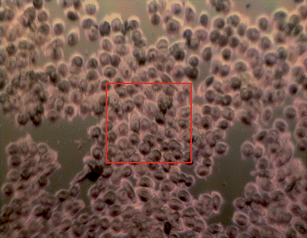 | ||
| Fig. 2 RWPE-1 cultured cells on a MirrIR slide with the aperture area 150 × 150 µm2 shown by the red square. | ||
Data analysis
Two different analyses were performed. The datasets acquired using synchrotron and laboratory based microspectroscopy were analysed in a typical fashion i.e. with the analyst choosing the pre-processing procedures and multivariate model to use, whereas the laboratory based broadbeam spectroscopic study was analysed using genetic algorithm fed support vector machines and principal component analysis. For the microspectroscopic study the cell lines used were RWPE-1, RWPE-2, WPE1-NA22, WPE1-NB26 and WPE1-NB11. The broadbeam spectroscopic study used these cell lines as well as WPE1-NB14.The spectral range 900–1800 cm−1 was used, resulting in 467 spectral data points for principal component analysis (PCA) and principal component–discriminant function analysis (PC–DFA). PCA is a common unsupervised multivariate method for finding patterns/structures within high dimensionality datasets. PCA was computed using the Non-linear Iterative Partial Least Squares (NIPALS) algorithm. PC–DFA utilises PCA to reduce the dimensionality of the data prior to discriminant function analysis (DFA). DFA then discriminates between groups on the basis of the resultant PCs and the a priori knowledge of the group membership that are fed into the DFA algorithm. Maximising the inter-group variance and minimising the intra-group variance achieve this. The maximum number of discriminant functions available is the number of groups minus one.20 The optimum number of PCs was determined iteratively. Prior to DFA, the dataset was split into a training set and an independent test set. The spectra were randomly assigned to either set, with the constraint that 20% of the spectra collected on each cell line should belong to the independent test set. As PC–DFA is a supervised technique and the model is supplied with information about group membership, any result produced by the model needs to be tested. This testing was carried out by supplying the model with the independent test set and observing where the model places the spectra on a graphical output. Confidence ellipses or ellipsoids are added to the discriminant function plots. These are, respectively, 2D and 3D visualisation of the 95% confidence interval. This was achieved using error_ellipse.m written by A. J. Johnson and obtained from Matlab central file exchange.21 Covariance matrices were calculated from the discriminant function analysis score matrix for each grouping, where the centroid was defined as the mean of each discriminant function analysis score matrix for each grouping.
| Cell line | Training set | Validation set | Test set | Total |
|---|---|---|---|---|
| a Number of cultures shown in brackets. | ||||
| RWPE-1 | 150 (15) | 30 (3) | 120 (12) | 300 (30) |
| RWPE-2 | 150 (15) | 30 (3) | 100 (10) | 280 (28) |
| WPE1-NA22 | 150 (15) | 30 (3) | 70 (7) | 250 (25) |
| WPE1-NB11 | 150 (15) | 30 (3) | 110 (11) | 290 (29) |
| WPE1-NB14 | 150 (15) | 30 (3) | 70 (7) | 250 (25) |
| WPE1-NB26 | 150 (15) | 30 (3) | 60 (6) | 240 (24) |
The blind test set was used as a double blind set as the analysis was performed at the Focas Research Institute, Dublin, Ireland and the identity of the spectra in the blind test set was kept by MJB.
The genetic algorithm (GA), principal component analysis (PCA), support vector machine (SVM) and implementation of pre-processing functions were carried out using Matlab™. All analyses were performed using a dual quad core (Zenon) with 16 GB RAM.
Genetic algorithm (GA) implementation. A GA was used to discover the optimum pre-processing technique from a range of pre-processing techniques (Table 2). Optimisation was implemented using a modified version of the Genetic Algorithm Optimisation Toolbox for Matlab™.22
| Processing | Type | Range |
|---|---|---|
| Derivatisation | None | NA |
| 1st Order | NA | |
| 2nd Order | NA | |
| Smoothing | Savitzky–Golay 5th order | 5 7 9 11 13 15 17 19 21 |
| Moving average | 3 5 7 9 11 13 15 17 19 | |
| Scaling | Auto-scaling | NA |
| Range-scaling | NA | |
| EMSC | NA | NA |
50 independent genetic algorithm runs were conducted retaining the highest cross-validation score, which depends upon the number of correctly classified spectra in the validation set. Using the optimum solution from each independent run, a support vector machine (SVM) was trained using the selected pre-processing regimes and selected SVM meta-parameters. Jarvis and Goodacre have successfully demonstrated the genetic algorithm optimisation approach for the selection of pre-processing methods and discriminatory spectral regions.23
Support vector machine (SVM) implementation. Support vector machines were constructed using the LibSVM package.24 Binary versions of LibSVM's svmtrain and svmpredict programs were controlled from Matlab™.
Results and discussion
Invasion assay
The results of the invasion assay towards tissue culture plastic (TCP, blue) or bone marrow stroma (BMS, red) are shown in Fig. 3.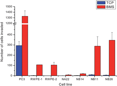 | ||
| Fig. 3 Graph showing the propensity of the different cell lines for invasion towards tissue culture plastic (TCP, blue) and bone marrow stroma (BMS, red). | ||
The invasion towards TCP is very low as expected, whereas when a strong chemoattractant such as BMS is introduced the invasive abilities of the cells are revealed. Bone is the most common metastatic site for prostate cancer and as such bone marrow stromal cells have been shown to enhance prostate cancer cell invasions.25 The invasiveness of the cell line is compared to the invasiveness of PC-3, a cell line established from a bone metastatic site.26 Previous studies have shown a range of invasiveness for these cell lines; RWPE-1 was found to be non-tumourigenic/invasive whilst WPE1-NA22, WPE1-NB14, RWPE-2, WPE1-NB11 and WPE1-NB26 displayed increasing tumourigenic and invasive characteristics. The results of our invasion assay (Fig. 3), importantly, show RWPE-1 and the slow growing/tumour forming RWPE-2 to have about equal invasiveness capacity towards BMS and the WPE1 cell lines follow the general increase as reported in the literature, however, the error bars of the WPE1-NB11 and WPE1-NB26 cell lines do overlap significantly.
Laboratory based and synchrotron based microspectroscopic study
The PCA score plot is shown in Fig. 4. Utilising the first two principal components (PCs) yielded the best separation of the cell lines, PC1 accounted for 56% and PC2 21% of the variance. Explaining 8% of the variance, PC3 did not provide any better separation.
 | ||
| Fig. 4 PCA score plot of the whole dataset (PC1 vs. PC2). A different coloured circle as per the legend of the figure represents each spectrum of the cell lines. | ||
Spectra from the RWPE-1 cell line (yellow circles) formed the most discernible cluster. PC1 generally separates the non-tumourigenic RWPE-1 and low invasiveness cell line WPE1-NA22 from the slow tumour forming RWPE-2 and the more invasive cell lines (WPE1-NB11 and WPE1-NB26), whereas PC2 generally separates RWPE from WPE cell lines. Observing both PC1 and PC2 together, three distinct groupings can be seen: (1) RWPE-1, (2) RWPE-2 and WPE1-NA22 and (3) WPE1-NA11 and WPE1-NB26. However, as the clusters are not wholly clear, a supervised method of multivariate analysis, such as PC–DFA, will be used to illuminate difference between the cell lines.
Fig. 5(A) shows the discriminant function plot of DF1 vs. DF2 for the multiple cell spectral model based upon the training set (coloured filled circles) and independent test set (coloured empty squares), as per the figure legend, with a 95% confidence limit drawn and Fig. 5(B) shows the discriminant function plot of DF1 vs. DF3 with the 95% confidence limit drawn. The discrimination in the plots shows different separations based upon different characteristics with Fig. 5(A) showing discrimination along DF1 based upon genetic (RWPE) versus genetic plus chemical (WPE1) transformation and DF2 has separated two different types of genetic transformation, HPV-18 for RWPE-1 compared with HPV-18 plus Ki-Ras for RWPE-2. Fig. 5(B) shows the same separation along DF1 however DF3 is separating WPE1-NA22 from WPE1-NB11 and WPE1-NB26. However, it is not clear if this separation is based upon invasiveness or the difference in amount of MNU used to achieve the chemical transformation.
 | ||
| Fig. 5 Discriminant function plots showing (A) DF1 vs. DF2 and (B) DF1 vs. DF3 for the multiple cell spectral model based upon the training set (coloured filled circles) and independent test set (coloured empty squares), as per the figure legend, with a 95% confidence ellipse drawn. | ||
As 3 discriminant functions have been used it was relevant to use a pseudo-3D discriminant function plot. Fig. 6(A) shows a 3D discriminant function plot of DF1 vs. DF2 vs. DF3 based upon the training set data (coloured filled circles) and independent test set (coloured empty squares), as per the figure legend.
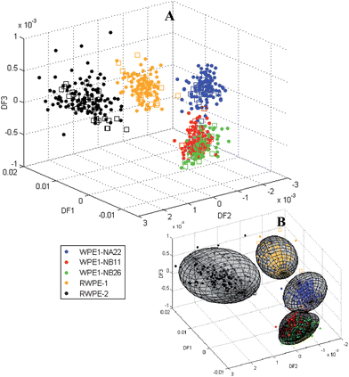 | ||
| Fig. 6 (A) Pseudo-3D discriminant function plot of DF1 vs. DF2 vs. DF3 based upon the training set (coloured filled circles) and independent test set (coloured empty squares) and (B) pseudo-3D discriminant function plot with 95% confidence ellipsoids. | ||
To assess the quality of discrimination the measures of sensitivity and specificity are used. Sensitivity measures the ability of the model to correctly classify whereas specificity measures the ability of the model to not misdiagnose. The sensitivities and specificities for the multiple cell spectral model based upon the pseudo-3D discriminant function plot are shown in Table 4.
| Cell line | True positives | False negatives | Sensitivity (%) | True negatives | False positives | Specificity (%) |
|---|---|---|---|---|---|---|
| RWPE-1 | 23 | 4 | 85.2 | 108 | 0 | 100.0 |
| RWPE-2 | 29 | 1 | 96.7 | 105 | 0 | 100.0 |
| WPE1-NA22 | 25 | 0 | 100.0 | 109 | 1 | 99.1 |
| WPE1-NB11 | 27 | 2 | 93.1 | 87 | 19 | 82.1 |
| WPE1-NB26 | 22 | 2 | 91.7 | 86 | 25 | 77.5 |
| WPE1(NB11 + 26) | 50 | 3 | 94.3 | 82 | 0 | 100.0 |
The sensitivities and specificities (Table 4) and the pseudo-3D discriminant function plot (Fig. 6) reveal that all the false positives for WPE1-NB11 were from WPE1-NB26 spectra and all the false positives for WPE1-NB26 were from the WPE1-NB11 spectra. Due to this, a new group comprising of cells from both cell lines was tested for sensitivity and specificity. Invasion assay results (Fig. 3) show that WPE1-NB26 and WPE-NB11 are very close in their invasiveness. The pseudo-3D model is able to discriminate 4 groups of cell lines RWPE-1, RWPE-2, WPE1-NA22 and WPE1-NB(11 and 26), to a high degree of accuracy, with the average sensitivity and specificity of 94% and 99.8% respectively. The specificity was exceptional in illuminating the robustness of the discrimination. Test spectra which did not fall within the confidence ellipsoid did not fall into the wrong ellipsoid.
Discriminant function 1 separated the RWPE cell lines from the WPE1 cell lines whilst discriminant functions 2 and 3 provide separation within these two groups (Fig. 5 and 6). The model is able to adequately differentiate cell lines from the RWPE and WPE families. Clusters corresponding to the chemically modified cell lines lay close to each other and the more aggressive clusters (WPE1-NB11 and WPE1-NB26) clustered together. WPE1-NA22 cells were derived from cells exposed to MNU at a concentration of 50 µg l−1 whereas WPE1-NB11 and WPE1-NB26 originated from the same batch of cells exposed to MNU at 100 µg l−1 and were separated from each other only after successive steps of growth in culture and injection into immunodeficient mice.7 Although, cell lines are separated, there is no systematic order of separation according to level of invasiveness and thus it appears to be primarily dependent on the method of transformation rather than the difference in invasiveness which raises questions on the usefulness of cell lines in modelling cancer. Erukhimovitch et al.27 have previously questioned the use of cell lines to model non-malignant cells in their study on human and mouse cell lines, cancer cells and primary cells. This study suggests that cell lines should all be considered as premalignant cells due to the immortal character achieved by the transformation. Our study takes this further by suggesting that biochemical changes induced by different transformation methods are primarily responsible for the discrimination of the RWPE family of cell lines and it is not possible, as was the research aim, to model biochemical changes associated with invasiveness using FTIR spectroscopy in prostate cancer using these cell lines.
A study by Romeo et al.1 on human oral mucosa cells and canine cervical cells resulted in the different cell types grouping together. This was thought to be due to the nucleus to cytoplasm ratio of the cells being more discriminatory than biochemical changes. However, a recent study28 has shown that the major reason for discrimination of prostate cancer cell lines, albeit ones from different anatomical positions, by FTIR is the biochemical differences between the cell lines. Thus we can be confident that we are observing discriminatory biochemical differences between the RWPE family of cell lines but it should be stressed that these differences appear to derive from the method of transformation rather than the degree of invasiveness.
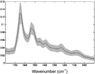 | ||
| Fig. 7 The average spectrum (black) ± standard deviation (grey) of the whole single-cell spectral dataset after vector normalisation and EMSC correction and of the spectral range 900–1800 cm−1 used for analysis. | ||
To assess the preliminary data collected on single cells a PC–DFA analysis was performed. However, in this analysis instead of splitting the data into a training set and independent test set 10 separate analyses were performed with 7 randomly chosen spectra from each cell line in the training set and the remaining spectra in the independent test set each time. Fig. 8(A) shows a pseudo-3D discriminant function plot of DF1 vs. DF2 vs. DF3 based upon one of the ten analyses performed with the training set data (coloured filled circles) and independent test set (coloured empty squares). Fig. 8(B) shows the discriminant function plot with 95% ellipsoids drawn.
 | ||
| Fig. 8 (A) Pseudo-3D discriminant function plot of DF1 vs. DF2 vs. DF3 based upon the training set (coloured filled circles) and independent test set (coloured empty squares) and (B) pseudo-3D discriminant function plot with 95% confidence ellipsoids. | ||
Spectra from the preliminary single-cell model did not cluster as well as the multiple cell spectra. Spectra from RWPE-1 and RWPE-2 are clearly distinguishable from each other along discriminant function 2 and from the WPE1 cell lines along discriminant function 1, whereas the WPE1 cell lines are less distinguishable. Due to the increased variability in the spectra and the small size of the dataset, 95% confidence ellipsoids were large and overlapped. The average sensitivities and specificities for the single-cell model are shown in Table 5.
| Cell line | Sensitivity (%) | Specificity (%) |
|---|---|---|
| RWPE-1 | 27.1 | 87.1 |
| RWPE-2 | 60.0 | 93.7 |
| WPE1-NA22 | 70.6 | 78.6 |
| WPE1-NB11 | 88.6 | 66.6 |
| WPE1-NB26 | 90.0 | 73.1 |
The overall average sensitivity and specificity are 67.3% and 79.8%, respectively, for this preliminary single-cell dataset. The model was able to adequately separate RWPE-1 from RWPE-2 and the RWPE cell lines from WPE1 cell lines.
The results from the preliminary single-cell spectral model are consistent with those from the multiple cell spectral model in that the same 3 main clusters consisting of HPV-18 transformed RWPE-1, HPV-18 and Ki-ras transformed RWPE-2 and HPV-18 and chemically transformed WPE1 cells are isolated. However, discrimination between the WPE1 cells could not be achieved. The standard deviation observed among the single-cell spectra was larger than that observed for the multiple spectra, attesting the large variability between single cells. A study by German et al. utilising synchrotron and laboratory based infrared radiation has shown that both techniques highlight similar spectral characteristic despite the increased intra-variability observed with synchrotron FTIR microspectroscopy.29 Importantly this preliminary study on single cells has concurred with the multiple cell spectral study, which was performed on a different instrument with a different experimental protocol and on a different scale.
Laboratory based broadbeam spectroscopic study
| A | |||||||
|---|---|---|---|---|---|---|---|
| Derivatisation | EMSC | Filter type | Window | Normalisation | Scaling | SVM penalty (C) | RBF gamma |
| 1st order | None | MA | 9 | None | Auto | 9.6017 | 9.6626 |
| B | ||||||||
|---|---|---|---|---|---|---|---|---|
| IR assignment | RWPE-1 | RWPE-2 | WPE-NA22 | WPE-NB11 | WPE-NB14 | WPE-NB26 | Sensitivity (R) | |
| Actual Cell Line | RWPE-1 | 108 | 1 | 10 | 0 | 1 | 0 | 90.00 |
| RWPE-2 | 0 | 100 | 0 | 0 | 0 | 0 | 100.00 | |
| WPE-NA22 | 0 | 0 | 69 | 0 | 0 | 1 | 98.57 | |
| WPE-NB11 | 0 | 0 | 0 | 110 | 0 | 0 | 100.00 | |
| WPE-NB14 | 0 | 0 | 0 | 0 | 67 | 3 | 95.71 | |
| WPE-NB26 | 0 | 0 | 0 | 0 | 0 | 60 | 100.00 | |
| Specificity (S) | 100.00 | 99.70 | 97.83 | 100.00 | 99.78 | 99.15 | ||
The genetic algorithm fed SVM is able to discriminate the RWPE family of cell lines to an average overall sensitivity and specificity of 97.37% and 99.41% respectively. The main errors in the model arise from RWPE-1 cells misclassified as WPE1-NA22 and WPE1-NB14 misclassified as WPE1-NB26. Although these misclassifications are small in number they are important since they are to cell lines with very different degrees of invasiveness.
As the imagined end user of these technologies will not be a spectroscopist or chemometrician and the ultimate aim is to translate this research into the clinical environment it is necessary to generate a robust set of pre-processing functions into which the pathologist can easily input spectral data and acquire a clinically relevant output. The use of genetic algorithms (GAs) to select pre-processing conditions and/or discriminatory regions of the spectrum can allow this research community to provide a standard list of options which are acceptable to be supplied to the GA and hence allow optimum separation.
 | ||
| Fig. 9 PCA score plot of the dataset processed using the optimum GA chosen pre-processing methods (PC1 vs. PC2). A different coloured circle as per the legend of the figure represents each spectrum of the cell lines (ellipses drawn as a guide to the eye). | ||
Observing the score plot (Fig. 9) for the GA fed SVM, it can again be seen that the groups are not differentiating on invasiveness of the cell line but appear similar to the PC–DFA results obtained on the laboratory based microspectrometer study with a differentiation being made between the RWPE cell lines (genetically transformed) and the WPE1 cell lines (genetically and chemically transformed) along PC1. General clustering can be seen for all cell lines apart from WPE1-NA22.
Conclusions
Laboratory based and synchrotron based microspectroscopic study
FTIR microspectroscopy has been used to distinguish between cells derived from the same origin, same anatomical position, having a close genetic background but differing on tumourigenic behaviour and as such we have further demonstrated the use of FTIR as a sensitive tool for evaluating biological samples and processes. The discrimination has been achieved to a high degree of classification accuracy and repeated with a preliminary study on single cells. The differentiation classification accuracy is better within the laboratory based study compared to the synchrotron based study, primarily due to significantly higher variance in single-cell data and the smaller datasets available. It should be remembered, however, that the single-cell data provide information concerning cell populations and not just the average which can be a significant advantage. The model presented here, however, discriminates based upon differences between the way these closely related cell lines have been transformed and not their invasiveness, showing their unsuitability to model prostate cancer using FTIR and raising important questions on the use of cell lines as cancer models.Laboratory based broadbeam spectroscopic study
This study has shown the use of a genetic algorithm to select optimum pre-processing methods. This allows us to determine the pre-processing methods which can be used whilst allowing the determined end user maximum flexibility in the application of the technologies and methods concerned with this research. Importantly it has also validated discrimination results observed in the other studies presented in this paper.Overall, the study demonstrates the potential of FTIR coupled with multivariate analysis technique for pathological screening applications although further studies involving primary cells and tissue are clearly required. The use of genetic algorithms (GAs) to selecting pre-processing conditions and/or discriminatory regions of the spectrum can allow the research community to provide a standard list of options which are acceptable to be supplied to the GA and hence allow optimum separation. Once all the issues regarding spectral correction and pre-processing have been resolved there is no reason why this technology cannot be used routinely in a clinical environment to augment current practice.
Acknowledgements
The authors would like to acknowledge the EPSRC Life Science Interface Scheme (grant reference: EP/E039855/1) and MIMIT™ (Manchester: Integrating Medicine and Innovative Technology) for financial support.References
- M. Romeo, B. Mohlenhoff, M. Jennings and M. Diem, Biochim. Biophys. Acta, 2006, 1758, 915–922 CAS.
- E. Gazi, J. Dwyer, P. Gardner, A. Ghanbari-Siahkali, A. P. Wade, N. P. Lockyer, J. C. Vickerman, N. W. Clarke, J. H. Shanks, L. J. Scott, C. A. Hart and M. Brown, J. Pathol., 2003, 201, 99–108 CrossRef.
- P. Crow, N. Stone, C. A. Kendall, J. S. Uff, J. A. M. Farmer, H. Barr and M. P. J. Wright, Br. J. Cancer, 2003, 89, 106–108 CrossRef CAS.
- T. J. Harvey, C. Hughes, A. D. Ward, E. Correia Faria, A. Henderson, N. W. Clarke, M. D. Brown, R. D. Snook and P. Gardner, Biophotonics, 2009, 2, 47–69 Search PubMed.
- T. J. Harvey, E. Correia, E. Gazi, A. D. Ward, N. W. Clarke, M. D. Brown, R. D. Snook and P. Gardner, J. Biomed. Opt., 2008, 13, 064004 CrossRef.
- D. Bello, M. M. Webber, H. K. Kleinman, D. D. Wartinger and J. S. Rhim, Carcinogenesis, 1997, 18(6), 1215–1223 CrossRef CAS.
- M. M. Webber, S. T. Quader, H. K. Kleinmann, D. Bello-DeOcampo, P. D. Storto, G. Bice, W. DeMendonca-Calaca and D. E. Williams, Prostate, 2001, 47(1), 1–13 CrossRef CAS.
- R. K. Sahu and S. Mordechai, Future Oncol., 2005, 1(5), 635–647 Search PubMed.
- E. Gazi, J. Dwyer, N. Lockyer, J. C. Vickerman, J. Miyan, C. A. Hart, M. Brown, J. H. Shanks and N. Clarke, Faraday Discuss., 2004, 126, 41–59 RSC.
- E. Gazi, M. Baker, J. Dwyer, N. P. Lockyer, P. Gardner, J. Shanks, R. S. Reeve, C. A. Hart, N. W. Clarke and M. D. Brown, Eur. Urol., 2006, 50, 750–761 CrossRef.
- M. J. Baker, E. Gazi, M. D. Brown, J. H. Shanks, P. Gardner and N. W. Clarke, Br. J. Cancer, 2008, 99(11), 1859–1866 CrossRef CAS.
- P. Lasch, W. Haensch, E. Neil Lewis, L. H. Kidder and D. Naumann, Appl. Spectrosc., 2002, 56, 1–9 CrossRef CAS.
- P. Lasch, M. Diem, W. Haensch and D. Naumann, J. Chemom., 2007, 20, 209–220.
- B. R. Wood, L. Chiriboga, H. Yee, M. A. Quinn, D. McNaughton and M. Diem, Gynaecol. Oncol., 2004, 93, 59–68 Search PubMed.
- E. Gazi, J. Dwyer, N. P. Lockyer, P. Gardner, J. Miyan, C. A. Hart, M. D. Brown, J. H. Shanks and N. W. Clarke, Biopolymers, 2005, 77, 18–30 CrossRef CAS.
- C. A. Hart, M. Brown, S. Bagley, M. Sharrad and N. W. Clarke, Br. J. Cancer, 2005, 92, 503–512 CAS.
- H. Martens, J. Pram Nielsen and S. Balling Engelsen, Anal. Chem., 2003, 75(3), 394–404 CrossRef CAS.
- P. Bassan, H. J. Byrne, F. Bonnier, J. Lee, P. Dumas and P. Gardner, Analyst, 2009, 134, 1586–1593 RSC.
- P. Bassan, A. Kohler, H. Martens, J. Lee, H. J. Byrne, P. Dumas, E. Gazi, M. Brown, N. Clarke and P. Gardner, Analyst, 2010, 135, 268–277 RSC.
- W. R. Klecka, Discriminant Analysis (Quantitative Applications in the Social Science), Sage Publications, Beverly Hills, CA, USA, 1st edn, 1980 Search PubMed.
- Matlab Central File exchange, http://www.mathworks.com/matlabcentral/fileexchange/4705, accessed 3rd September 2009.
- C. Houck, J. Joines and M. Kay, A genetic algorithm for function optimization: a Matlab implementation, North Carolina State University, Raleigh, NC, 1995 – Technical Report NCSU-IE-TR-95-09 Search PubMed.
- R. M. Jarvis and R. Goodacre, Bioinformatics, 2005, 21(7), 860–868 CAS.
- C. C. Chang and C. J. Lin, LIBSVM: a library for support vector machines, 2001, http://www.csie.ntu.edu.tw/%7Ecjlin/libsvm.
- H. Ide, T. Yoshida, N. Matsumoto, K. Aoki, Y. Osada, T. Sugimura and M. Terada, Cancer Res., 1997, 57, 5022–5027 CAS.
- M. E. Kaighn, K. S. Narayan, Y. Ohnuki, J. F. Lechner and L. W. Jones, Invest. Urol., 1979, 17(1), 16–23 Search PubMed.
- V. Erukhimovitch, M. Talyshinsky, Y. Souprun and M. Huleihel, Photochem. Photobiol., 2002, 76(4), 446–451 CrossRef CAS.
- T. J. Harvey, E. Gazi, A. Henderson, R. D. Snook, N. W. Clarke, M. Brown and P. Gardner, Analyst, 2009, 134, 1083–1091 RSC.
- M. J. German, A. Hammiche, N. Ragavan, M. J. Tobin, L. J. Cooper, S. S. Matanhelia, A. C. Hindley, C. M. Nicholson, N. J. Fulwood, H. M. Pollock and F. L. Martin, Biophys. J., 2006, 90(10), 3783–3795 CrossRef CAS.
| This journal is © The Royal Society of Chemistry 2010 |