Ethanol fuel use in Brazil: air quality impacts

Abstract

Brazil has a long history in the development of ethanol for use as a liquid fuel for vehicles. They have developed one of most efficient and economical systems for producing ethanol in the world. Brazil provides an example that many other countries would like to emulate. Using ethanol as a vehicle fuel has significant potential air quality impacts. This paper will review the available air quality and vehicle emissions data in Brazil, specifically focusing on vehicle related pollutants that may be impacted by the use of large quantities of ethanol in the fuel. The atmospheric concentrations of acetaldehyde (CH₃CHO) and ethanol in Brazil are much higher than those in other areas of the world, while the concentrations of the single ring aromatic compounds and small carboxylic acids are more typical of observations elsewhere. Acetaldehyde and ethanol increase in vehicle emissions and nitrogen oxides (NO_x) may increase when ethanol fuels are used. Both CH₃CHO and NO_x are very important contributors to photochemical air pollution and ozone (O₃) formation. There are very significant O₃ air quality problems in Brazil, most studied in the larger cities of São Paulo and Rio de Janeiro. These are issues that must be evaluated for other areas of the world that are considering the use of high ethanol content vehicle fuels.

---

Broader context

Brazil has a long history of using ethanol as a vehicle fuel, and has developed one of most efficient and economical systems for producing ethanol in the world. Brazil is an example that many other countries would like to emulate. Using large quantities of ethanol as a vehicle fuel has significant potential air quality impacts. This paper will review the available air quality and vehicle emissions data from Brazil, specifically focusing on vehicle related pollutants that may be impacted by the use of large quantities of ethanol in the fuel. Acetaldehyde and ethanol emissions increase in vehicles using ethanol fuels, and the atmospheric concentrations of these compounds are higher than most other areas of the world. Nitrogen oxides emissions may also increase when ethanol fuels are used. Both acetaldehyde and nitrogen oxides are important contributors to photochemical air pollution and ozone formation. There are very significant ozone problems in and around the larger cities of São Paulo and Rio de Janeiro, Brazil. This review is intended to highlight issues that must be considered and evaluated for other areas of the world that are considering the use of high ethanol content vehicle fuels.

Introduction

Over the years, many articles have appeared in the popular press extolling the virtues of ethanol fuel use. Dickerson¹ has published one such article. The article suggests that Brazil is on a path to independence from foreign oil, by developing its own oil reserves and by investing heavily in renewable energy from ethanol. About 40% of the fuel Brazilians use in their vehicles is ethanol (ton of oil equivalent (toe) basis). In addition, we are told that “environmentalists support the expansion of this clean, renewable fuel that has helped improve air quality in Brazil's cities.” What do we really know about air quality in Brazil? In this paper, we will review the available data on the air quality and vehicle emissions in the only area of the world (Brazil) that has used high ethanol content fuels for many years. The issues discussed should be considered by other countries that are considering the use of high ethanol content fuels.

Niven² has recently reviewed the environmental impacts and sustainability of ethanol in gasoline. Niven reviews data available on five environmental aspects of using ethanol blended with gasoline as a vehicle fuel. These include: (1) the effects on the emissions of air pollutants during the use of these fuels; (2) the impact of the fuels on subsurface soils and groundwater; (3) the effects of blending ethanol with the fuels on greenhouse gas emissions; (4) the energy efficiency of ethanol; and (5) the overall sustainability of ethanol production. Much of the discussion focuses on the use of 10% by volume blends of ethanol with gasoline (E10), the most commonly used blend globally. The conclusion of this work was that “E10 is of debatable air pollution merit (and may in fact increase the production of photochemical smog); offers little advantage in terms of greenhouse gas emissions, energy efficiency or environmental sustainability; and will significantly increase both the risk and severity of soil and groundwater contamination.”² In order to supplant significant quantities of petroleum use as a vehicle fuel for light duty vehicles, high ethanol concentration blends such as 85% ethanol and 15% gasoline (E85) are the most likely alternative in the short term. Niven² goes on to conclude that “E85 offers significant greenhouse gas benefits, however, it will produce significant air pollution impacts, involves substantial risks to biodiversity, and its groundwater contamination impacts and overall sustainability are largely unknown.” These latter conclusions for the high ethanol content fuels are based on very little data, because little data are available. It is generally believed that high ethanol content fuels will have less impact on groundwater than the fuels that they replace. The greenhouse gas benefits of high ethanol content fuels is also subject to considerable added uncertainty due to the impacts of land-use changes.³

Jacobson⁴ has constructed a model to evaluate the air quality and related health impacts of E85 fuel use in southern California and the US. Jacobson⁴ concludes that ozone (O₃) would increase in southern California and the northeastern part of the US, which “may increase O₃ related mortality, hospitalization, and asthma by about 9% in Los Angeles and 4% in the US as a whole, relative to 100% gasoline. E85 also increased peroxyacetyl nitrate (PAN) in the US but was estimated to cause little change in cancer risk.” Furthermore, “because of the uncertainty in future emission regulations, it can be concluded with confidence only that E85 is unlikely to improve air quality over future gasoline vehicles.”⁴ In addition, “unburned ethanol emissions from E85 may result in a global scale source of acetaldehyde larger than that of direct emissions.” The results of this work increased the controversy surrounding ethanol fuel use.

History of ethanol fuel use in Brazil

The use of ethanol as fuel for automobile engines in Brazil started in the 1920s. The mandatory use of 5% ethanol with gasoline as a blend was established by the Government in 1931 both because of the decline in international sugar prices and because all of the gasoline consumed in the country was imported.⁵ In 1933, the Sugar and Alcohol Institute (IAA) was created with the goal of expanding alcohol production capacity in order to deal with the overproduction of sugar.⁵ During World War II, the use of alcohol increased due to gasoline rationing. The use of alcohol declined in the 1950s and 1960s due to rising sugar prices, the decline in gasoline prices and PETROBRAS (Brazilian Petroleum Company) achieving self-sufficiency in oil refining.⁵

In the early 1970s, Brazil's exports of sugar increased dramatically, with international sugar prices reaching a peak in November 1974.⁵ This was followed by a long and pronounced decline in sugar prices. At about the same time there was a sharp increase in oil prices which threatened the military dictatorship's ability to rule.^6,7 At that time 90% of the gasoline was imported, causing fuel shortages, inflation, and diminished hard currency reserves. In November 1975, the National Alcohol Program (PNA), commonly known as “ProAlcool”, was set up to use domestic sources as a substitute for imported petroleum. The goal was to allow continued energy consumption and maintain economic growth.⁸ The program required use of 10% anhydrous ethanol as an additive to gasoline, with a voluntary component using 100% hydrated ethanol (95% ethanol + 5% water) in modified Otto cycle engines.⁷ During the first few years of the program, the objective was to install distilleries adjacent to existing sugar mills to produce anhydrous ethanol to be blended with gasoline.⁸

By 1979, the international oil crisis forced the Brazilian government to launch a second phase of the PNA. The goal was to use hydrous ethanol to completely substitute gasoline in automobiles.⁵ Agreement was reached between the government and automobile industry that allowed the program to proceed. With strong Government oversight, new distilleries were constructed for the large scale production of hydrous ethanol.⁸ This shift from anhydrous ethanol to hydrous ethanol production and the scale of the substitution had important repercussions on the balance of payments, on the automobile market, on oil refining and on the agricultural sector.⁵Fig. 1 shows new light duty vehicle production in Brazil as related to fuel used. This figure dramatically illustrates the growth in hydrous ethanol fueled vehicle production during the 1980s.

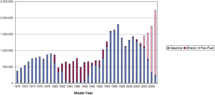Fig. 1 New light duty vehicle sales (non-diesel) by fuel type: gasoline (including gasohol), ethanol (hydrous) and flex fuel. Source: http://www.unica.com.br/downloads/estatisticas/eng/VEHICLES SALES IN BRAZIL.xls.

Between 1975 and 1985, the production of sugarcane quadrupled and alcohol became a very important fuel used in the country.⁹ In 1984, the new civilian administration (the first after the military regime) cut public investment and subsidies.⁸ Due to the PNA program, about 94% of the new passenger vehicles were fueled by ethanol. By the late 1980s serious problems had developed. Large off-shore oil and natural gas reserves were discovered in the south and in the northeast of the country. There was a large drop in gasoline and fuel oil consumption in Brazil between 1973 and 1985 that was not easily accommodated by the refineries (see Fig. 2). As a result one-third of gasoline production, and one-fourth of fuel oil production, had to be exported at low prices. During 1989–1990 the surplus of gasoline, together with a combination of factors—economic recession; high inflation and alcohol producer debts; international debt crisis; the increase of international prices of sugar; the continued fall in international prices of petroleum; the lack of a coherent strategy for balancing the supply and demand for alcohol and gasoline; and the reduction in part of the subsidies to the program—national alcohol production changed from overproduction to a situation of deficit production.⁵ In 1990, a combination of bad climatic conditions together with a rise in the international price of sugar forced the Government to import alcohol (including methanol) for the first time to meet the national demand.⁵ Consumers had serious difficulties in getting alcohol to fill the tanks of their cars. In that year the production of alcohol-powered cars dropped from about 47% of new cars produced, to about 11%.

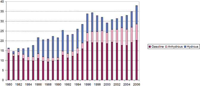Fig. 2 Annual production (in 10⁶ m³ year⁻¹) of gasoline, anhydrous ethanol and hydrous ethanol in Brazil. Source: ref. 8, http://www.unica.com.br/and and http://www.anp.gov.br/.

In 1993, the government passed a law in which all gasoline marketed in Brazil would be blended with 20–25% of ethanol.⁶ In 1994 the Plan Real was launched with the objective of stabilizing the Brazilian economy and reducing inflation rates to single digits. The Federal Government policy was to force the sugar and ethanol industry to cut costs through higher productivity.⁸ In 1995 only 2.5% of all new cars were fueled by ethanol, but 35% (4.2 million) of the total number of cars were still powered with ethanol engines, the remaining 65% using a blend of ethanol with gasoline in amounts of about 22% ethanol.⁵ In 1995 Brazilian ethanol production again did not meet the national demand.⁵ In that year, 13.1 billion litres of alcohol were produced from 62% of the sugarcane crop and 1.8 billion litres of alcohol were imported, 40% as methanol and 60% as ethanol.

At the end of 1995, the Government officially launched the program, now called ‘new PNA’.⁵ Its new goal is to protect the environment, not to reduce oil dependence. Sugarcane prices, including freight to mills and distilleries, and all ethanol prices were deregulated and determined by market forces starting 1 January 1997.⁶ A special investment program was made available as an incentive for the continuation and the expansion of ethanol fuel production, to increase the research and production of new and improved engines, to reduce ethanol production costs, to increase the productivity of the ethanol industries and to reduce the amount of wastes.⁵

Currently the government's role in ethanol fuels is much less and much different than in earlier times. Its role is to ensure that the market-driven controls proceed smoothly, and to help improve the industry's environmental performance.⁶ Problems continue with the competition between the food and fuels sectors for sugarcane. In March 2006, the country's fuel blenders (e.g. BR (PETROBRAS), Shell, Exxon, Ipiranga) had to cut ethanol content to 20% of its blended fuel because of ethanol shortages.⁶ Sugar prices had risen to their highest levels in five years.

In March 2003, flexible (flex) fuel vehicles were introduced into the market in Brazil (see Fig. 1). These vehicles are designed to be fueled with gasohol, or ethanol, or any blend of gasohol and ethanol. For the customers, the value of the flex fuel vehicle is to allow the choice of fuel (each time the vehicle is refueled) according to characteristics of price, quality, performance and fuel availability. The vehicle uses special electronic sensors and an on-board computer to recognize the fuel composition and properly adjust the engine combustion parameters, without any interference from the driver. Fig. 1 shows the rapidly increasing importance of the flex fuel vehicle in Brazil's new car market.

Vehicle emissions

Vehicle emission standards

In the late 1980s, Brazil adopted regulations on vehicle emissions. The Vehicle Air Pollution Control Program (PROCONVE) established emission standards for new vehicles in Brazil. Table 1 shows the emissions limits set for new gasoline/ethanol fueled automobiles in Brazil.

Table 1 Light duty vehicle emissions limits (PROCONVE)^5,10–12

Pollutant^a	Phase I	Phase II	Phase III	Phase IV	Phase V
	1988	1992	1997	2007	2009
a CO—carbon monoxide; HC—hydrocarbon; NMHC—non-methane hydrocarbon; NOx—nitrogen oxides; PM—particulate matter.
CO/g km^−1	24.00	12.00	2.00	2.00	2.00
HC/g km^−1	2.10	1.20	0.30	0.30	0.30
NMHC/g km^−1	—	—	—	0.16	0.05
NOx/g km^−1	2.00	1.40	0.60	0.25	0.12
PM/g km^−1	—	—	0.05	0.05	0.05
Aldehyde/g km^−1	—	0.15	0.03	0.03	0.02
Evaporative/g test^−1	6.00	6.00	6.00	2.00	2.00

---

The addition of ethanol to gasoline increases the octane rating of gasoline, prevents pre-ignition, and can be used as a replacement for the tetraethyl lead additive used in gasoline.⁵ The widespread introduction of unleaded fuels throughout Brazil in 1975 allowed the level of lead in the air in urban areas to decrease by about 72% by the mid-1990s.¹³

Vehicle emission measurements

The vehicle emissions data described in this work are those which are available in the open literature. These data may not be representative of results that would be applicable to vehicles in widespread use.

Onursal and Gautam¹² have presented data for the average emissions of new light duty vehicles in the São Paulo metropolitan region. The vehicle emissions data show that the average emissions for the new vehicles are substantially below the emissions standards. The average carbon monoxide (CO) emissions for the gasohol fueled vehicles are higher than for the ethanol fueled vehicles. The hydrocarbon (HC) and nitrogen oxides (NO_x) emissions are nearly the same for both fuel types, and the average aldehyde emissions are considerably higher for the ethanol fueled vehicles compared to gasohol. For the ethanol fueled vehicles, the HC emissions were about 70% ethanol, 10% aldehydes and 20% other organics, while for gasohol vehicles, the HC emissions were less than 10% each of ethanol and aldehydes, and more than 80% of the emissions were other organics. The aldehyde emissions from ethanol fueled vehicles were about 85% CH₃CHO, 14% formaldehyde (CH₂O) and 1% other aldehydes, while for gasohol vehicles CH₂O was about 60% of the aldehyde emissions. These data have been updated and extended to model year 2007 vehicles, as shown in Table 2.¹⁴ Emissions data from flex fuel vehicles are included for the most recent years.

Table 2 Average emissions for new light duty vehicles in the São Paulo metropolitan region^12,14

Model year	Fuel type	Exhaust emissions/g km^−1				Evaporative/g test^−1
		CO	HC	NOx	Aldehydes
a na—not available.
Pre-1980	Gasoline	54.0	4.7	1.2	0.050	na^a
1980–1983	Ethanol	18.0	1.6	1.0	0.160	na^a
	Gasohol	33.0	3.0	1.4	0.050	na^a
1984–1985	Ethanol	16.9	1.6	1.2	0.180	10.0
	Gasohol	28.0	2.4	1.6	0.050	23.0
1986–1987	Ethanol	16.0	1.6	1.8	0.110	10.0
	Gasohol	22.0	2.0	1.9	0.040	23.0
1988–1989	Ethanol	13.1	1.6	1.3	0.110	10.0
	Gasohol	16.9	1.6	1.7	0.040	23.0
1990–1991	Ethanol	9.6	1.2	1.1	0.110	1.8
	Gasohol	12.4	1.4	1.4	0.040	2.7
1992–1993	Ethanol	3.9	0.6	0.6	0.038	1.0
	Gasohol	6.2	0.6	0.7	0.018	1.9
1994–1995	Ethanol	4.6	0.7	0.7	0.042	0.9
	Gasohol	5.4	0.6	0.6	0.030	1.6
1996–1997	Ethanol	2.4	0.5	0.5	0.026	1.0
	Gasohol	2.5	0.3	0.4	0.013	1.1
1998–1999	Ethanol	0.63	0.18	0.23	0.014	1.48
	Gasohol	0.77	0.17	0.27	0.006	0.80
2000–2001	Ethanol	0.64	0.16	0.15	0.015	1.33
	Gasohol	0.60	0.12	0.17	0.004	0.70
2002–2003	Ethanol	0.75	0.16	0.09	0.018	na^a
	Gasohol	0.41	0.11	0.12	0.004	0.68
2004–2005	Ethanol	0.82	0.17	0.08	0.016	na^a
	Gasohol	0.35	0.10	0.07	0.004	0.69
	Flex-eth	0.42	0.14	0.12	0.014	na^a
	Flex-gas	0.42	0.10	0.05	0.003	na^a
2006	Ethanol	0.67	0.12	0.05	0.14	na^a
2006–2007	Gasohol	0.33	0.08	0.08	0.002	0.46
	Flex-eth	0.47	0.11	0.07	0.014	1.27
	Flex-gas	0.48	0.10	0.05	0.003	0.62

---

Emissions measurements have been made on two different three-way catalyst equipped cars (1980 GM Opala and 1982 VW Gol) operating on hydrated ethanol.^15,16 Acetaldehyde is the major carbonyl emission from these vehicles, contributing 88–99% of the sum of CH₂O and CH₃CHO emitted during different phases of the emissions tests for the two vehicles. The mass emissions for the GM Opala were 0.046 g km⁻¹ and 0.246 g km⁻¹ for CH₂O and CH₃CHO without a catalyst, and 0.014 g km⁻¹ and 0.044 g km⁻¹ with the catalyst installed. The emissions from the VW Gol were 0.019 g km⁻¹ and 0.143 g km⁻¹ for CH₂O and CH₃CHO without a catalyst, and 0.005 g km⁻¹ and 0.023 g km⁻¹ with the catalyst installed. On a molar basis the CH₂O/CH₃CHO ratio in emissions were 0.26 and 0.19 without the catalyst, and 0.45 and 0.30 with the catalyst.¹⁷

Coutrim et al.¹⁸ have reported emissions from two test engines without catalysts for aldehydes from ethanol blended fuels. One test engine was fueled with an ethanol rich fuel (82% hydrous ethanol with 18% gasoline) and the second with gasohol (22% anhydrous ethanol with 78% gasoline). The higher ethanol fueled engine produced about 1.7 times as much CH₂O and 3.5 times as much CH₃CHO as did the gasohol engine. The molar CH₂O/CH₃CHO ratio for these two fuels was 0.42 for the ethanol rich fuel, and 0.86 for the gasohol fuel.

Correa et al.¹⁹ performed emissions tests on three ethanol fueled vehicles (1992, 1994, and 1995 model years) and three gasohol fueled vehicles (1996, 1997, and 2000 model years) running at a constant 800 rpm. The ethanol fueled vehicles are older which is typical of this portion of the vehicle fleet. The molar CH₂O/CH₃CHO ratio in emissions from the ethanol fueled vehicles was 0.68, and 0.75 for the gasohol fueled vehicles. In these tests, the emissions of aldehydes were lower for the older ethanol fueled vehicles than for the newer gasohol fueled vehicles.

Sales and Sodre²⁰ modified the cold start system for an ethanol fueled vehicle in an attempt to reduce exhaust emissions for the vehicle. It was found the HC and CO emissions could be reduced by up to 8.6 and 17.2% and allowed a faster start with the implementation of changes in the cold start system. Essentially no change in NO_x and aldehyde emissions was found as a result of these tests. The average emissions from this 1.0 L four-cylinder engine-powered vehicle operated on the FTP-75 test cycle ranged from 1.68 to 1.84 g km⁻¹ for HC, from 7.29 to 8.80 g km⁻¹ for CO, from 0.34 to 0.35 g km⁻¹ for aldehydes, and from 1.32 to 1.36 g km⁻¹ for NO_x for the four test configurations studied in this work.

Lucon et al.²¹ have presented CETESB (the state environmental agency in São Paulo) emissions data for model year 2003 and 2004 new vehicles. These vehicles consisted of three types: conventional vehicles designed for gasohol use; conventional vehicles designed for ethanol use; and flex fuel vehicles. The flex fuel vehicles were tested on both gasohol and ethanol. Since conventional vehicles that operate on ethanol fuels are such a small part of the new vehicle market, comparisons of emissions of flex fuel vehicles with the two different fuels with conventional gasohol vehicles will be discussed. The emissions of HC, NO_x and total aldehydes were lower for flex fuel vehicles operating on gasohol than conventional gasohol vehicles by 41%, 56% and 12% respectively, but CO emissions were higher by 18%. For the flex fuel vehicles operating on ethanol compared to conventional gasohol vehicles, the emissions of CO, HC and NO_x increased by 30–36%, while the total aldehyde emissions increased by an average of over 300%. The average emissions for all of these new vehicles are lower than the emissions standards for these vehicles. The fuel economy of flex fuel vehicles operating on gasohol was about 6% lower, and operating on ethanol was about 37% lower, than for conventional vehicles operating on gasohol.

de Abrantes et al.²² have reported results of the measurements of emissions of polycyclic aromatic hydrocarbons (PAHs) from vehicles fueled with gasohol and with ethanol. The average emissions of PAHs from gasohol fuel use were higher than those with ethanol fuel use, averaging 0.832 µg TEQ km⁻¹ (BAP eq) (TEQ—toxicity equivalences; BAP eq—benzo(a)pyrene equivalences) for the gasohol tests and 0.016 µg TEQ km⁻¹ (BAP eq) for the ethanol tests. Fuel additives and oil composition had a significant effect on PAH emissions with the gasohol fuel, but no significant effect with ethanol fuel.

Diesel vehicles contribute significantly to the total vehicle emissions and hence to air quality in Brazil. de Abrantes et al.^23,24 present results of standard dynamometer FTP-75 emissions tests on four Brazilian light duty diesel vehicles. The average CH₃CHO emission for two tests on all four vehicles was 15.5 mg km⁻¹ and the average CH₂O emission was 43.2 mg km⁻¹. For these diesel vehicle emissions tests the average molar CH₂O/CH₃CHO ratio was 3.9. All of the vehicles tested met the vehicle emissions standards for the years they were produced, but none met the 2009 aldehyde emission standard of 20 mg km⁻¹. The CH₂O/CH₃CHO emissions ratios from diesel vehicles in Brazil are much higher that the corresponding ratios for gasohol and ethanol fueled vehicles. Molar ratios of CH₂O/CH₃CHO are used throughout this paper to aid in identifying the source of these compounds, from emissions and in the ambient air.

Correa and Arbilla have reported results of aromatic HC²⁵ and carbonyl²⁶ emissions with diesel and biodiesel fuels from a heavy duty diesel engine typical of that used in buses in Brazil. The fuels tested were commercial diesel, and 2%, 5%, and 20% (B2, B5, B20) biodiesel blends with diesel. The biodiesel was made by esterification of castor oil with ethanol. The use of the biodiesel blends led to significant reductions in the emissions of the monocyclic aromatic HCs, including the BTEX compounds (benzene, toluene, ethylbenzene and xylenes), by about 5%, 9% and 22% relative to the diesel fuel. Similar reductions in PAH emissions were found with increasing concentration of biodiesel. The tests for effects on carbonyl emissions included a 10% (B10) biodiesel blend in addition to the fuels identified above.²⁵ The emissions of the aliphatic carbonyl compounds increased systematically with increasing biodiesel in the blends. Guarieiro et al.²⁷ have found different results from their study of carbonyl emissions from diesel and biodiesel blends. The fuels studied ranged from pure diesel to pure biodiesel. The data show no significant trend in the CH₂O emissions as fuel composition changed, but CH₃CHO emissions decreased slightly with increasing biodiesel. The sampling techniques for carbonyl compounds used in this study were different than the previous study and these tests were conducted on a small two-cylinder diesel engine. In addition, the biodiesels used were different—a methyl soy biodiesel and a methyl residual oil biodiesel.

Merritt et al.²⁸ have reported emissions measurements from ethanol–diesel blends. This may become an important petroleum substitute in Brazil, but there are some technical barriers that must be overcome prior to its use. The test data were collected from three non-road diesel engines using a base diesel fuel, and diesel fuel blended with 7.7%, 10% and 15% ethanol by volume. Formaldehyde emissions for the three ethanol blended fuels increased slightly by an average of 3.6%, 6.7% and 22%, while CH₃CHO emissions increased by an average of 41%, 57% and 104% respectively. The only other emissions to change significantly were those of ethanol which was the largest of the measured emissions, and it increased in proportion to the quantity of ethanol blended with the fuel. The emissions of benzene decreased slightly with increasing ethanol, but other aromatic HC emissions varied both up and down.

Compressed natural gas (CNG) is a fuel that is being used in increasing quantities as a vehicle fuel in Brazil. Many CNG vehicles are dual fueled vehicles which can use CNG or gasohol. Correa and Arbilla²⁹ performed emissions tests on 20 of these dual fueled vehicles operating at a constant 2500 rpm. When natural gas was used as the fuel, the average CH₂O/CH₃CHO ratio was 3.42. When these same vehicles were run on gasohol fuel, the average CH₂O/CH₃CHO ratio was 0.24. Consistently, the CNG fueled test emitted more CH₂O and less CH₃CHO than the gasohol fuel test.

Martins et al.³⁰ have reported the results of extensive measurements of CO, CO₂, NO_x, sulfur dioxide (SO₂) and individual HC and carbonyl compounds both inside and outside of tunnels in São Paulo, Brazil. Samples were collected in the Janio Quadros Tunnel during late March 2004 and in the Maria Maluf Tunnel in early May 2004. On average 95% of the vehicles passing through the Janio Quadros Tunnel use either gasohol or hydrous ethanol, with the remaining vehicles being light duty vehicles burning diesel fuel. On average 13% of the vehicles using the Maria Maluf Tunnel are heavy duty diesel fueled, with the remaining fueled by gasohol or hydrous ethanol. These data were used to determine emission factors for various compounds from the vehicle fleet. For the light duty vehicles the emissions factors for CO and NO_x were found to be 14.6 ± 2.3 g km⁻¹ and 1.6 ± 0.3 g km⁻¹ respectively, while for the heavy duty vehicles these emissions factors were found to be 20.6 ± 4.7 g km⁻¹ and 22.3 ± 9.8 g km⁻¹ respectively. The average emission factors for the following organic compounds in the Maria Maluf Tunnel were: CH₂O 48.4 ± 35.1 mg km⁻¹; CH₃CHO 45.7 ± 29.1 mg km⁻¹; benzene 78.3 ± 72.0 mg km⁻¹; toluene 134.5 ± 135.4 mg km⁻¹; ethylbenzene 31.1 ± 33.0 mg km⁻¹; m,p-xylene 62.0 ± 62.8 mg km⁻¹; and o-xylene 44.4 ± 39.8 mg km⁻¹. The average molar CH₂O/CH₃CHO ratio in emissions from these vehicles is 1.5.

Teixeira et al.³¹ have done an evaluation of mobile source emissions for the metropolitan area of Porto Alegre. This work shows that gasohol fueled vehicles contribute the largest portions of CO and HC emissions, while diesel vehicles contribute the largest portions of NO_x, sulfur oxides (SO_x) and particulate emissions. Gasohol and ethanol fueled vehicles are the major contributors to aldehyde emissions. This study generated total annual vehicle emissions for these pollutants from the early 1980s through to 2004. The emission of CO, NO_x, HC and particulates showed a significant growth through the early 1990s, followed by a gradual decline from the mid-1990s through to 2004. It was also shown that aldehyde emissions increased gradually through the entire period. The average emissions for ethanol fueled vehicles in 2004 exceeded the emissions standards for CO and HC, while the average emissions of diesel vehicles exceeded the emissions standards for NO_x.

The CETESB³² has presented average emissions data for the fleet of vehicles operating on gasohol and ethanol in the São Paulo metropolitan region. For the fleet of gasohol fueled vehicles the average CO emissions decreased from about 17 g km⁻¹ in 1997 to about 11 g km⁻¹ in 2006, the average HC emissions decreased from about 1.5 g km⁻¹ in 1997 to about 1.1 g km⁻¹ in 2006, and the average NO_x emissions decreased from about 0.9 g km⁻¹ in 1997 to about 0.7 g km⁻¹ in 2006. During this same time period for the fleet of ethanol fueled vehicles the average CO emissions increased from about 16 g km⁻¹ to 20 g km⁻¹ by 2006, the average HC emissions increased from about 1.9 g km⁻¹ to 2.1 g km⁻¹ by 2006, and the average NO_x emissions increased from about 1.1 and 1.3 g km⁻¹ between 1997 and 2006. These data show that the fleet average emission rates for CO, HCs and NO_x for the ethanol fueled vehicles are higher than those from the gasohol fueled fleet. As can be seen from Fig. 1, very few new ethanol fueled vehicles have been sold since 1997, hence this portion of the fleet is getting older and many of the old ethanol fueled vehicles are still in the fleet. The gasohol fueled portion of the fleet has continued to grow with the addition of new gasohol-powered vehicles. Domingues and Gatti³³ have reported some speciated volatile organic compound (VOC) data for emissions from gasohol vehicles, analyzing 75 individual VOC compounds. They found that the top ten VOC compounds in emissions (excluding the carbonyl compounds) were: toluene; p-xylene; 2-methylbutane; 2,2,3,3-tetramethyl-butane; benzene; pentane; ethane; 1,3-butadiene; m-xylene and o-xylene.

A recent emission inventory (2005) for the city of São Paulo concluded that CH₃CHO and CH₂O account for 3% and 4% respectively of the VOC emissions.²⁵ The recent increases in the emissions of these compounds may be due to the use of ethanol, gasohol and natural gas fuels, but the increased use of biodiesel may also be contributing to these emissions changes.^19,26,29

Air quality effects

Romieu et al.³⁴ discuss some of the early air quality impacts of increased use of ethanol fuels in São Paulo, Brazil. About 84 000 cars used ethanol fuel in 1981 which increased to about 500 000 by 1985. At the same time there was an 18.2% decrease in the number of vehicles using gasoline. The main impacts on air quality indices due to the shift in fuel consumption were: decreased SO₂; maximum CO values tended to be lower, but still exceeded standards at all monitoring locations; lead in the air decreased from 1 µg m⁻³ in 1978 to 0.3 µg m⁻³ in 1983.³⁴ More recently, the annual average concentrations of lead in São Paulo ranged from a high of 0.17 µg m⁻³ to a low of 0.06 µg m⁻³ at the four sites monitored during 1997 and 2003.¹⁴ It was suggested that O₃ exposure may not be properly assessed in the early years due to the small number of monitoring stations in the area. The high levels of HCs, the levels of nitrogen dioxide (NO₂) and geographical factors suggest high production of oxidants. Romieu et al.³⁴ suggested that the shift towards increased ethanol fuel use increases the emissions of aldehydes to the air which could lead to an increase in O₃ production.

Gurjar et al.³⁵ have evaluated emissions and air quality in 18 mega-cities, based on World Bank and United Nations data. They have used a multi-pollutant index based on three criteria pollutants: total suspended particulates (TSP), SO₂, and NO₂. Two of the mega-cities in this evaluation are in Brazil—São Paulo and Rio de Janeiro. Based on this multi-pollutant index, Rio de Janeiro ranks as the 12th most polluted and São Paulo ranks as the 17th most polluted. None of the pollutants in this index are part of the specific discussions of air quality impacts of ethanol fuel use.

In this paper, atmospheric measurements will be reported that are available in the open literature. These measurements may include very small data sets, widely varying sampling locations, sampling periods and seasonality, and differing sampling and analysis techniques. These differences will make it difficult to compare results from these studies.

Atmospheric aldehydes

The results of early measurements of total aldehyde concentrations in São Paulo have been reported.³⁶ These measurements of total aldehydes were made using the 3-methyl-2-benzothiazolinone hydrochloride (MBTH) method. This method measures total aldehydes, not individual compounds. The concentration results are presented as CH₂O. Long-term monitoring was reported for four sites in São Paulo. This long-term monitoring consisted of 24 h sampling periods on weekdays (Monday–Friday) at each of the four sites from July 1980 to June 1981. The average concentrations of the total aldehydes reported at each of these sites over the year are shown in Table 3. The Praça do Correio and Congonhas sites are believed to be more heavily influenced by primary aldehydes, directly emitted from motor vehicles, since the mean CO concentrations were highest at these two sites. These concentrations are quite high compared to measurements in other areas of the world. Table 3 summarizes the measurements of CH₂O and CH₃CHO made in the São Paulo area.

Table 3 Summary of ambient CH₂O, CH₃CHO and CH₂O/CH₃CHO ratio data in São Paulo, Brazil

Month/year	Location	CH2O/ppb	CH3CHO/ppb	CH2O/CH3CHO ratio	Number of samples	Sample period/h	Ref.^a
a Thesis and CETESB refer to a thesis or CETESB report cited in the numbered reference.
Jul. 1980–Jun. 1981	Praça do Correio	Total aldehydes	42	—	∼260	24	36
Jul. 1980–Jun. 1981	Parque Dom Pedro	Total aldehydes	20	—	∼260	24	36
Jul. 1980–Jun. 1981	Mooca	Total aldehydes	15	—	∼260	24	36
Jul. 1980–Jun. 1981	Congonhas	Total aldehydes	27	—	∼260	24	36
Oct. 1986	Praça do Correio	5.4	16.1	0.3	3	2	39
Jun.–Jul. 1988	Univ. São Paulo	8.8	7.6	2.5	8	2–4	39
Jul. 1988	CETESB	13.5	8.1	2.2	4	1.5	39
Dec. 1988	Congonhas	14.5	24.2	0.6	26	—	Thesis-50
1988	—	16.3	30.6	0.5	47	—	Thesis-61
Jul. 1989	—	4.5	10.5	0.4	32	—	Thesis-61
Sep.–Oct. 1989	Congonhas	10.8	22.3	0.5	17	—	CETESB-50
Mar.–Apr. 1990	Cerqueira César	15.5	24.3	0.6	23	—	CETESB-50
Apr. 1990	Mooca	8.5	16.2	0.5	12	—	CETESB-50
Aug. 1990	Cerqueira César	21.8	27.3	0.8	6	—	CETESB-50
Jan. 1993	Six locations	7.8	11.3	0.7	6	3–8	40
1993	Mooca	4.2	6.1	0.7	179	—	CETESB-50
1993	Cerqueira César	7.6	10.6	0.7	180	—	CETESB-50
Oct. 96–Jan. 97	Cerqueira César	5.4	7.5	0.7	132	—	CETESB-50
Oct. 96–Jan. 97	Univ. São Paulo	1.3	2.8	0.5	60	—	CETESB-50
Jan.–Jul. 1997	Several sites	9	10	—	39	3	46
Jul.–Sep. 1997	Cerqueira César	7.0	11.7	0.6	155	—	CETESB-50
Jul.–Sep. 1997	Univ. São Paulo	4.2	9.2	0.5	130	—	CETESB-50
Feb. 1998	Univ. São Paulo	5	5.4	0.9	11	1	47
Aug. 1999	Água Funda	12.3	11.3	1.3	32	2	49
Aug. 1999	Cidade Universitária	13.9	12.5	1.2	34	2	49
Nov. 2000	Univ. São Paulo	4.2	—	—	18	2	51
Aug. 2001	Janio Quadros Tunnel	24–31	34–35	0.9	—	2	52
Aug. 2001	Ambient-Janio Quadros	3.3–46	1.2–57	1.4	—	2	52
Oct. 2001	Maria Maluf Tunnel	28–39	25–32	1.0	—	2	52
Oct. 2001	Ambient-Maria Maluf	1.0–46	4.2–51	1.4	—	2	52
Aug. 2002	Univ. São Paulo	4.0	—	—	30	1	51
Mar.–Apr. 2004	Fourteen locations	18.1	15.4	1.2	14	1	59
Jul.–Oct. 2006	Cerqueira César	5.7	5.6	1.0	141	2	32
Feb. 2007	Univ. São Paulo	13.5	—	—	5	2	51

---

Tanner et al.³⁷ have reported results of CH₂O and CH₃CHO measurements made using the 2,4-dinitrophenylhydrazine (DNPH) coated cartridge technique. Twelve-hour samples were collected for a four day period (1–5 July, 1985) at the Vila Isabel site in Rio de Janeiro, Brazil. In addition, 1- or 2-h samples were collected at this site on 2 and 4 July, and at the Pontifical Catholic University of Rio de Janeiro (PUC/RJ) site on 9 July. The CH₂O and CH₃CHO concentrations for Rio de Janeiro are shown in Table 4. For the 12 h data, the nighttime average ratio of CH₂O/CH₃CHO = 0.57 ± 0.12, which was lower than the daytime ratio of 0.80 ± 0.07. This nighttime ratio agrees well with the ratio of CH₂O/CH₃CHO = 0.60 ± 0.02 measured in the Santa Barbara Tunnel in Rio de Janeiro during April 1985. The average of the 1 h and 2 h daytime aldehyde concentration measurements made at the Vila Isabel site were much higher than the daytime average concentration measurements made at the PUC/RJ site. The measurements at this site were influenced by a strong sea-breeze, and were much lower than data collected at the downtown site, but still well above the marine background levels reported by Lowe and Schmidt³⁸ in the south Atlantic. These results suggest that aldehyde concentrations, particularly CH₃CHO, are increased considerably by additional primary emission sources in Rio de Janeiro that are not common in other countries. These sources are likely to be ethanol fueled and gasohol fueled motor vehicles.

Table 4 Summary of ambient CH₂O, CH₃CHO and CH₂O/CH₃CHO ratio data in Rio de Janeiro, Brazil

Month/year	Location	CH2O/ppb	CH3CHO/ppb	CH2O/CH3CHO ratio	Number of samples	Sample period/h	Ref.^a
a Thesis and Conf. refer to a thesis or conference report cited in the numbered reference. b Period when the sample was collected is not stated in the reference.
Apr. 1985	Santa Barbara Tunnel	10.6	17.1	0.6	8	—	37
Jul. 1985	Villa Isabel	9.8	13.5	0.7	7	12	37
Jul. 1985	Villa Isabel	26	37	0.7	15	1–3	37
Jul. 1985	Gávea (PUC)	1.8	3.7	0.5	10	1–2	37
Jan. 1987	Gávea	4.6	6.2	0.8	2	—	Thesis-50
Jan. 1987	Santa Barbara Tunnel	65	236	0.3	2	1	39
Jan. 1987	Rebouças Tunnel	154	307	0.5	1	—	Thesis-61
Sep. 1987	R. Cosme Velho	4.1	4.7	0.9	6	2–7	39
Jan. 1993	Six locations	9.7	28	0.5	6	6–8	40
Dec. 1995	One location	11.8	9.9	1.2	11	6	42
1997??^b	Prédio Centro	5.8	6.3	—	—	—	Conf.-43
1997??^b	FIOCRUZ	2.7	9.3	—	—	—	Conf.-43
Dec. 1998	Av. Presidente Vargas	19.5	21.2	1.0	4	2	19
1998??^b	FIOCRUZ	4.0	2.7	—	—	—	Conf.-43
Aug. 1999	Av. Presidente Vargas	3.4	4.9	0.7	15	2	19
May–Nov. 2000	Av. Presidente Vargas	8.8	5.8	1.5	13	2–3	50
Aug.–Nov. 2000	Av. Presidente Vargas	16.8	15.3	1.2	6	2–3	19
Jan. 2001	Av. Presidente Vargas	51	41	1.2	3	2	19
Aug.–Dec. 2001	Av. Presidente Vargas	52	38	1.4	6	3	29
Feb.–Dec. 2002	Av. Presidente Vargas	68	15.8	4.7	18	1.5–3	29
Apr.–Nov. 2002	FIOCRUZ	132	35	4.0	45	2	54
Apr. 2002–Feb. 2003	Tijuca District	151	30	4.9	86	2	55
Dec. 2003	Eight locations	10.1	11.1	0.9	8	1	58
Nov. 2005–Aug. 2006	Bus, air-conditioned	39	32	1.6	6	—	60
Nov. 2005–Aug. 2006	Bus station	118	89	1.4	5	—	60
2008	Praça Saens Peña	53.0	16.9	3.1	28	2	63
2008	Entrada Floresta da Tijuca	22.7	6.9	3.3	40	2	63
2008	Interior Floresta da Tijuca	9.4	3.1	3.0	40	2	63
2008	Alto Floresta da Tijuca	13.1	4.5	2.9	34	2	63

---

Grosjean et al.³⁹ present results of carbonyl sampling studies during the late 1980s using DNPH coated cartridges conducted at three sites in São Paulo, two sites in Rio de Janeiro, and one site in Salvador. The results of these measurements made in the different areas of Brazil are presented in Table 3 for São Paulo, Table 4 for Rio de Janeiro and Table 5 for Salvador. The sampling was done during the winter and early spring to minimize the contribution of photochemistry, and one of the sites in Rio de Janeiro was in a tunnel which would be more representative of on-road vehicle emissions. It was concluded³⁹ that CH₂O concentrations measured in Brazil are as high as those measured elsewhere in the world, but not substantially higher, while CH₃CHO concentrations were substantially higher, and the CH₂O/CH₃CHO ratio was consistently lower than that measured elsewhere. Furthermore, the tunnel data clearly show very high levels of vehicle emissions of CH₃CHO compared to CH₂O. The very high ambient concentrations of CH₃CHO are likely due to the large scale use of ethanol as a vehicle fuel.

Table 5 Summary of ambient CH₂O, CH₃CHO and CH₂O/CH₃CHO ratio data in other urban areas of Brazil

Month/year	Location	CH2O/ppb	CH3CHO/ppb	CH2O/CH3CHO ratio	Number of samples	Sample period/h	Ref.
a Period when the sample was collected is not stated in the reference.
Salvador
Sep. 1988	Vitoria street	8.9	19	0.5	3	1	39
1993??^a	Bus station	18.5	5.8	4.5	12	1	41
Feb. 1992	Tunnel	80	75	1.1	4	1	41
Jan. 1992	Bus station	52	12	4.4	11	1–2	44
1995??^a	Mall park-enclosed	8.3	13	0.7	5	1–2	44
1995??^a	Business park-enclosed	44	69	0.7	7	1–2	44
1995??^a	Tunnel	80	72	1.2	4	1–2	44
Apr. 1992	Rio Vermelho	2.9	3.5	1.0	17	1–2	44
Dec. 1991	Baixa dos Sapateiros	11	6.3	1.8	24	1–2	44
1995??^a	Lagoa Verde	1.5	2.1	0.8	17	1–2	44
1995??^a	Cacha-Pregos	1.2	1.2	1.1	20	1–2	44
Porto Alegre
Apr. 1997	Rodoviaria	15.7	17.7	0.9	6	1	45
Apr. 1997–Apr. 1999	Rodoviaria-morning	7.2	3.5	2.26	111	3	48
Apr. 1997–Apr. 1999	Rodoviaria-evening	5.0	3.0	1.75	22	3	48
May–Sep. 1999	Rodoviaria-morning	4.6	3.85	1.25	24	3	48
May–Sep. 1999	Rodoviaria-evening	4.8	4.7	1.07	21	3	48
Fortaleza
2003	Federal Univ. of Ceará	18.2	15.4	1.2		2	56
Nov.–Dec. 2004	Federal Univ. of Ceará	2.3	0.4	4	12	1.5–2	57
Londrina
Jan.–Feb. 2002	Bus station	7.9	1.3	6.3	14	24	53
Jan.–Feb. 2002	Central	4.1	3.0	1.4	16	24	53
Jul. 2002	Central	5.1	5.7	0.9	15	24	53
Jul. 2002	Agricultural	1.0	0.4	2.5	14	24	53

---

Several authors have reported measurements of CH₂O and CH₃CHO made both in indoor and outdoor air.^{40,42,46,56,57,60} The outdoor data collected in these studies and measurements made in bus stations and parking garages are included in the data tables (Tables 3, 4 and 5).

de Andrade et al.⁴¹ have reported the measurements of both gas phase and aerosol phase CH₂O and CH₃CHO in two source rich areas of Salvador, Brazil: (1) a bus station where the predominant traffic is diesel fueled buses; and (2) a tunnel where about 41% of the traffic is fueled by hydrous ethanol, about 50% by gasohol (approx. 22% ethanol) and about 8% by diesel fuel. The gas phase CH₂O and CH₃CHO concentrations measured in the bus station averaged 18.5 ppb and 5.8 ppb, while the aerosol concentrations averaged 0.014 µg m⁻³ and 0.038 µg m⁻³ for n = 12 samples. The gas phase CH₂O and CH₃CHO concentrations measured in the tunnel averaged 79.5 ppb and 75.0 ppb, while the aerosol concentrations averaged 0.163 µg m⁻³ and 0.060 µg m⁻³ for n = 4 samples. This work confirmed that more than 99% of the CH₂O and CH₃CHO are present in the gas phase. The gas phase CH₂O/CH₃CHO ratio for the bus station data was 4.5 ± 3.0 and for the tunnel was 1.1 ± 0.2 (Table 5). The high CH₂O/CH₃CHO ratio in the bus station is due to the much higher emissions of CH₂O from the diesel fueled buses.

de Andrade et al.⁴⁴ have reported results for measurements of CH₂O and CH₃CHO at six sites in Salvador, a fishing village and rural area in the vicinity of Salvador. There is no indication in the paper when these measurements were made. Four of the sites were enclosed. One of these was a bus station which served diesel fueled buses. The average concentration for CH₂O was 52 ppb, for CH₃CHO was 12 ppb, and the average CH₂O/CH₃CHO ratio was 4.4. Sampling was done in an enclosed mall parking lot and an enclosed business parking lot. For the mall lot, the average concentration of CH₂O was 8.3 ppb, that for CH₃CHO was 13 ppb, and the average CH₂O/CH₃CHO ratio was 0.66. For the business lot the average concentration for CH₂O was 44 ppb, that for CH₃CHO was 69 ppb, and the average CH₂O/CH₃CHO ratio was 0.65. The traffic in the parking facilities were light duty vehicles, using ethanol blended fuels for which CH₃CHO emissions are more important. Sampling was done in a tunnel and the average CH₂O concentration was 80 ppb, the average CH₃CHO was 72 ppb, and the average CH₂O/CH₃CHO ratio was 1.2. This CH₂O/CH₃CHO ratio is consistent with a mix of 82% light duty and 18% heavy duty vehicles in the traffic counts for the tunnel. Sampling done in a residential area found an average CH₂O/CH₃CHO ratio of 1.0, while sampling done in a commercial area found an average ratio of 1.8. Sampling was also done in a rural area (Lagoa Verde) about 250 km from Salvador where the average CH₂O/CH₃CHO ratio was 0.8, and a fishing village (Cacha-Pregos) about 20 km from Salvador where the average ratio was 1.1. The authors concluded that the CH₂O/CH₃CHO ratio can be described fairly reliably by considering the vehicle fleet mix of heavy duty (diesel) vehicles and light duty (ethanol/gasohol) vehicles and the CH₂O/CH₃CHO ratio in emissions for these fuel types.⁴⁴

Nguyen et al.⁴⁷ have reported CH₂O and CH₃CHO measurements in São Paulo, Brazil and in Osaka, Japan. Aldehyde measurements were made in Osaka from May to December 1997, resulting in average CH₂O and CH₃CHO concentrations of 1.9 ppb and 1.5 ppb, and the average CH₂O/CH₃CHO ratio was 1.3. The São Paulo measurements were collected near the University of São Paulo campus on four days in February 1998. The average CH₂O and CH₃CHO concentrations were 5.0 ppb and 5.4 ppb respectively, and the average CH₂O/CH₃CHO ratio was 0.94. The use of the ethanol fuels in Brazil led to the higher CH₃CHO concentrations relative to CH₂O.

Grosjean et al.⁴⁸ have reported CH₂O and CH₃CHO concentrations for an extensive set of measurements from Porto Alegre (April 1997–September 1999). From April 1997 to April 1999, 82% of the light duty vehicle fleet was fueled by gasoline mixed with 15% methyl tert-butyl ether (MTBE), while the remaining 18% was fueled by hydrous ethanol. In April 1999, the MTBE blended fuel was replaced by the conventional gasohol fuel used throughout the remainder of Brazil, a mixture of 20–25% ethanol and gasoline. Grosjean et al.⁴⁸ had the unique opportunity to study the effects of this fuel change on the ambient atmospheric concentrations of CH₂O and CH₃CHO in Porto Alegre. As shown in Table 5, 3 h average concentrations were measured in the morning (0700–1000) and evening (1700–2000) periods both before and after the fuel change. The atmospheric concentrations are highly variable and do not show a large change, but the average CH₂O/CH₃CHO ratio does show a significant change from 2.26, when MTBE blended fuels were used, to 1.25 after the switch to gasohol for the morning samples, and a change from 1.75, when MTBE blended fuels were used, to 1.07 after gasohol fuels were used for the evening samples. These data make it clear that the CH₃CHO emissions increase relative to CH₂O emissions as the fuel changes from an MTBE blend to gasohol.

Montero et al.⁴⁹ have reported measurements of CH₂O and CH₃CHO at two sites in São Paulo during August 1999. Two-hour samples were collected on consecutive days during morning (0800–1000), midday (1200–1400) and evening (1600–1800) time periods. The average CH₂O/CH₃CHO ratio varied with the time period of the day: for the Água Funda site the ratio was 0.9, 1.3, and 1.6 for the morning, midday and evening periods, while for the Cidade Universitária site the ratio was 0.7, 1.3 and 1.5 for these same periods. These data suggest that the morning measurements are predominately affected by direct vehicle emissions, while the midday and evening measurements have significant contribution from photochemically generated aldehydes as well. The CH₂O/CH₃CHO ratio is lowest in the morning sampling period, and increases as the day progresses. This is consistent with faster photochemical production of CH₂O than CH₃CHO.⁴⁹

Correa et al.^19,29 have collected samples for CH₂O and CH₃CHO at a site in Rio de Janeiro from December 1998 to December 2002. There was an attempt to look for trends in the annual average data. Insufficient samples were collected under similar conditions to allow identification of a trend. They suggested that CH₂O concentrations increased and CH₃CHO remained largely unchanged.²⁹ This is consistent with the results of the small number of observations made in December through the years. Correa and Arbilla²⁹ present data suggesting that the number of vehicles converted from gasohol to dual fueled with CNG increased from about 2% to about 12% of the fleet operating in Rio de Janeiro between 1998 and 2002 with the much higher CH₂O/CH₃CHO ratio in emissions for CNG vehicles as discussed earlier. This may be contributing to the increase in CH₂O with relatively little change in CH₃CHO.

Grosjean et al.⁵⁰ collected a series of 3 h carbonyl samples during the morning rush hour from May to November 2000 at a downtown location in Rio de Janeiro. These samples were analyzed for up to 61 carbonyl compounds. The measurements were made at the FEEMA (state environmental agency in Rio de Janeiro) air monitoring site near Avenida Presidente Vargas. The average CH₂O concentration for these measurements was 8.8 ppb, the average CH₃CHO concentration was 5.8 ppb, and the average CH₂O/CH₃CHO ratio was 1.5. All of the other carbonyl compounds except acetophenone correlated well with CH₂O and CH₃CHO, suggesting similar sources. In this paper, it was noted that the CH₂O/CH₃CHO ratio has been increasing in more recent years. It was suggested that this is due to the fact that no new vehicles are being sold that run on pure ethanol, and that there is increasing use of gasohol fueled vehicles. This may change with higher ethanol content fuels used in flex fuel vehicles.

Vasconcellos et al.⁵² have reported the results of carbonyl measurements in tunnels and in the ambient air nearby during August and October 2001 in São Paulo. Only light duty vehicles are allowed to use the Janio Quadros Tunnel (JQT), while both light duty and heavy duty vehicles use the Maria Maluf Tunnel (MMT). Hence the JQT is used by gasohol and ethanol fueled vehicles and the MMT is used by gasohol, ethanol and diesel fueled vehicles. The CH₂O/CH₃CHO ratios in the tunnels averaged 0.9 for JQT and 1.0 for MMT and were slightly lower than the ambient samples near the tunnels which averaged 1.4. The higher CH₂O/CH₃CHO ratio in MMT than JQT is due to the larger fraction of emissions from the diesel vehicles allowed to operate in that tunnel.

Pinto and Solci⁵³ have reported atmospheric measurements of CH₂O and CH₃CHO at two urban and one rural site in the area of Londrina (population about 500 000). Londrina is located about 500 km west of São Paulo and about 800 km west of Rio de Janeiro. Measurements of CH₂O and CH₃CHO were reported for a central bus station site and at a downtown site during January and February 2002. The CH₂O/CH₃CHO ratio was 6.3 at the bus station, and 1.4 at the downtown site. The higher ratio at the bus station site is consistent with the much larger contribution of CH₂O from diesel vehicles. Measurements were also reported for the downtown site and at a rural site during July 2002. The CH₂O/CH₃CHO ratio was 0.9 at the downtown site, and 2.5 at the rural site. This paper suggests that secondary sources are the most important for both aldehydes in rural areas, while primary sources are relatively important in urban areas.

Martins et al.⁵⁵ have reported atmospheric measurements of aldehydes in the Tijuca district of Rio de Janeiro between April 2002 and February 2003. A total of 86 samples were collected and analyzed for CH₂O, CH₃CHO, propionaldehyde, butyraldehyde and pentanaldehyde. The average concentrations of CH₂O and CH₃CHO were found to be 151 ± 64 ppb and 30 ± 14 ppb and the average CH₂O/CH₃CHO ratio was 4.9. The CH₂O concentration and the CH₂O/CH₃CHO ratio are much higher than observed in most previous studies. The vehicular traffic in this area was mainly light duty vehicles which use hydrous ethanol (14.6%), gasohol (78%), and CNG (7.4%). Depending on the time of day, diesel fueled buses represent 7–20% of the fleet in this area. The higher CH₂O concentrations relative to CH₃CHO are believed to be due to the increased use of CNG as a fuel for light duty vehicles. The dominant aldehyde emitted from diesel fueled buses is also CH₂O. These results are similar to those reported in another area of Rio de Janeiro during a similar time period by Rodrigues et al.⁵⁴

de Andrade et al.⁶¹ reviewed data on atmospheric carbonyls through the 1990s. The range of concentrations measured for CH₂O and CH₃CHO in Brazil are similar to those measured elsewhere (largely in the US), but the average concentrations of both compounds are generally higher in Brazil. The differences between the measurements in Brazil and those elsewhere is more obvious in the CH₂O/CH₃CHO ratio which is often less than one, unlike that seen elsewhere in the world. This is due to the increased emissions of CH₃CHO when ethanol is a fuel component.

Carvalho et al.⁶² have studied the biogenic emissions of HCs and carbonyl compounds from trees in forested areas of São Paulo. The emissions of CH₃CHO from trees was the largest of all of the carbonyl compounds studied, being about 2.5 times the CH₂O emission in one case, and no CH₂O emission was detected in the other case. Biogenic contributions to carbonyl compounds in the atmosphere may be significant under some conditions.

The CETESB³² conducted an aldehyde measurement campaign between July and October 2006 at the Cerqueira César site in São Paulo. The average concentrations reported for the 141 samples of 2 h duration were 5.7 ppb for CH₂O and 5.6 ppb for CH₃CHO. These concentrations are somewhat lower than those reported at the same site during a similar time period in 1997, which found average concentrations of 7.0 ppb and 11.7 ppb, for CH₂O and CH₃CHO respectively.³² The analytical methodology changed, making the results for CH₂O not directly comparable to the earlier results.

Jorge et al.⁶³ have explored the relative importance of biogenic emissions of CH₂O and CH₃CHO from trees in forested areas of Rio de Janeiro. Samples were collected at four different sites: Praça Saens Peña, a heavy traffic area near the forest; the entrance to the forest; a scenic overlook in the forest and an additional interior site. The concentrations of CH₂O and CH₃CHO were highest where there was the most vehicle traffic. The CH₂O/CH₃CHO ratio decreased slightly at the lower traffic sites, possibly suggesting a slight increase in biogenic contributions to these compounds.

Some more recent papers^29,54,55 have reported ambient data with CH₂O/CH₃CHO ratios that are high (4–5). Most of the earlier data have a CH₂O/CH₃CHO ratio of 1.5 or less. It is clear from these papers that the cause for the increase in the CH₂O/CH₃CHO ratio was an increase in ambient CH₂O concentration, not a decrease in CH₃CHO. The average CH₂O is 68 ppb (n = 18),²⁹ 151 ppb (n = 86)⁵⁴ and 132 ppb (n = 45)⁵⁵ for 1.5–3 h average samples (Table 4). These very high concentrations have been observed at some sites in Rio de Janeiro, but not in the other areas. These concentrations are sufficiently high to be of significant concern. Some of the increase in CH₂O concentration may be related to the increase in diesel fuel production relative to gasoline in Brazil, and to the increased use of CNG. Between 1998 and 2007, diesel fuel production in Brazil increased at a rate of about 2.0% year⁻¹, while gasoline production only increased at a rate of about 0.4% year⁻¹.⁶⁴

Atmospheric ethanol

Schilling et al.⁶⁵ developed a continuous enzymatic–fluorimetric method for the measurement of ethanol in ambient air. This method was used for ambient measurements of ethanol in Cubatão in the state of São Paulo during May 1996. Cubatão is located near the coast about 50 km southeast of the city of São Paulo. The diurnal character of the ethanol concentration was found to peak in the morning 0900–1000 at an average concentration of about 80 ppb and again in the evening at about 1800 at an average concentration of about 65 ppb. The diurnal average concentration of ethanol was found to remain relatively high (30–40 ppb) even through the nighttime hours. Table 6 shows a summary of these data and other measurements of methanol and ethanol in urban areas of Brazil.

Table 6 Summary of ambient methanol and ethanol measurements in Brazilian cities

Month/year	Location	Methanol/ppb	Ethanol/ppb	Number of samples	Sample period	Ref.
a nd—not detectable; na—not available. b Can—Summa canister grab sample; Sorbent—sorbent tube integrated sample. c 1, 2 and 4 h samples. d 1 and 2 h samples. e 1 h sample.
Rio de Janeiro
1996–1997	Muniz Barreto St.	14.0	66.4	12	0.25–0.50 h	66
Jun. and Nov. 1999	Eight urban tunnels	nd^a	95.3	8	1 min	69
Jun. and Nov. 1999	Four underground parking	nd^a	371	4	1 min	69
Jun. 1999–May 2000	Thirteen locations	nd^a	26.4	13	1 min	70
May–Nov. 2000	(FEEMA) Av. Presidente Vargas	nd^a	16.4	6	1 min	71
Dec. 2003	Eight locations	nd^a	6.8	8	1 h	58
São Paulo
1996–1997	Rebouças	19.6	36.2	9	0.25–0.50 h	66
Feb. 1998	Univ. São Paulo	34.1	176	11	1 min	47
Nov. 1998	Cerqueira César	9.2	468	6	Can^b^,^c	68
Nov. 1998	Cerqueira César	nd^a	11	16	Sorbent^b^,^c	68
Nov. 1998	Ibirapuera Park	12.9	397	6	Can^b^,^c	68
Nov. 1998	Ibirapuera Park	5.9	60	16	Sorbent^b^,^c	68
Nov. 1998	Lapa	13.4	313	6	Can^b^,^c	68
Nov. 1998	Lapa	nd^a	103	12	Sorbent^b^,^c	68
Nov. 1998	Congonhas	6.4	526	6	Can^b^,^c	68
Nov. 1998	Congonhas	nd^a	43	6	Sorbent^b^,^c	68
Nov. 1998	Parque Dom Pedro	6.9	138	4	Can^b^,^d	68
Nov. 1998	Parque Dom Pedro	nd^a	16	4	Sorbent^b^,^d	68
Nov. 1998	Tunel 9 de Julho	12.6	1018	2	Can^b^,^e	68
Nov. 1998	Tunel 9 de Julho	nd^a	105	2	Sorbent^b^,^e	68
Mar.–Apr. 2004	Fourteen locations	nd^a	13.9	14	1 h	59
Salvador
1996–1997	Garibaldi Av.	9.8	65.4	21	0.25–0.50 h	66
1996–1997	Institute of Chemistry	nd^a (<7.6)	17.9	5	0.25–0.50 h	66
Porto Alegre
Mar. 1996–Apr. 1997	Rodoviaria	na^a	12.1	43	1 min	67
Apr. 1997	Rodoviaria	na^a	31.6	6	1 min	45
Cubatão
May 1996	Industrial complex	na^a	20–360	Continuous (11 day)	3 min	65
May 1996	Industrial complex	na^a	30–80	Diurnal average	1 h	65

---

Pereira et al.⁶⁶ have developed a technique using sorbent cartridge collection of alcohols, followed by extraction and gas chromatography-flame ionisation detector (GC-FID) analysis. Ambient samples were collected on florisil cartridges at sites in Rio de Janeiro, São Paulo and Salvador. For all of these samples the ethanol concentrations are much higher than methanol.

Grosjean et al.^45,67 have reported ambient measurements of ethanol for samples collected in Summa canisters in Porto Alegre between 1996 and 1997. The samples were analyzed by GC-mass spectrometry (MS) and GC-FID. During this period in the Porto Alegre area about 17% of the vehicles used hydrous ethanol fuel, 74% used a mixture of 85% gasoline and 15% MTBE and 9% were buses and trucks using diesel fuel without either ethanol or MTBE. All other areas of Brazil used gasohol instead of MTBE blended fuels. The ambient concentrations of ethanol ranged up to 68.2 ppb and averaged 12.1 ± 13.3 ppb.

Nguyen et al.⁴⁷ have reported methanol, ethanol and isopropanol measurements by the alkyl nitrite formation reaction and product analysis by GC-electron capture detector (ECD) in São Paulo, Brazil and in Osaka, Japan. Alcohol measurements were made in Osaka every 2 h for one day a month from May to December 1997. The average methanol and ethanol concentrations were 5.8 ± 3.8 ppb and 8.2 ± 4.6 ppb respectively. Eleven samples were collected for alcohol analysis near the University of São Paulo campus on four days in February 1998. The average methanol and ethanol concentrations were 34.1 ± 9.4 ppb and 176.3 ± 38.1 ppb respectively. The average ratio of ethanol/methanol in São Paulo during the summer measurements was 5.2, while the average of the summer measurements of this ratio in Osaka was 0.9. The atmospheric concentrations of ethanol reported for São Paulo were about 20 times higher than those for Osaka. The use of ethanol fueled vehicles in São Paulo has led to extraordinarily high atmospheric concentrations of ethanol in the air.

Colon et al.⁶⁸ collected and analyzed VOC samples from six different sites in São Paulo during November 1998. This was part of a joint USEPA and CETESB study of VOCs in São Paulo. For each sample day, samples were collected using sorbent tubes and also in Summa canisters. These samples were analyzed by GC-MS. It is believed that the alcohols were lost from the sorbent tubes during sample shipping prior to analysis. The methanol and ethanol concentrations were quantified in all of the canister samples. The VOC mix observed in São Paulo was dominated by ethanol. The methanol concentrations observed in the canisters in São Paulo are comparable to similar observations in the US, but the ethanol concentrations observed in São Paulo are about 40 times larger than previous observations in the US. This study should make the importance of measuring alcohol concentrations in the atmosphere quite clear.

Grosjean et al.⁶⁹ have reported VOC and ethanol concentration data for canister grab samples collected in eight tunnels and four underground parking garages during June and November 1999 in Rio de Janeiro. These samples were analyzed by GC-MS. Grosjean et al.⁷⁰ have reported VOC and ethanol concentration data for grab samples collected at 13 sites in Rio de Janeiro between June 1999 and May 2000. Grosjean et al.⁷¹ have reported VOC and ethanol concentration data for grab samples collected every two weeks at the FEEMA (state environmental agency) station near Avenida Presidente Vargas in Rio de Janeiro between May and November 2000.

Very limited data are available for ethanol concentrations in the atmosphere in Brazil. Ethanol concentrations of over 100 ppb were commonly reported in the urban areas where large quantities of ethanol were used.

Atmospheric BTEX

Gee and Sollars⁷² have reported some of the earliest measurements of benzene, toluene, ethylbenzene and xylenes (BTEX) compounds collected as 2 h samples on sorbent tubes and analyzed by GC-FID for São Paulo in 1995–1996. This study reported concentrations for several Latin American and Asian cities. Table 7 summarizes the measurements of the BTEX concentrations that have been reported for various urban areas in Brazil.

Table 7 Summary of ambient BTEX concentrations in urban areas of Brazil

Month/year	Location	B/ppb	T/ppb	E/ppb	m,p-X/ppb	o-X/ppb	Number of samples	Sample period	Ref.^a
a Rept—Report cited in numbered ref. b Total X—total xylenes. c nd—not detectable. d Can—Summa canister grab sample; Sorbent—sorbent tube integrated sample. e 1, 2 and 4 h samples. f 1 and 2 h samples. g 1 h sample.
Rio de Janeiro
Dec. 1995	One location	2.9	10.2	1.4	Total X^b	3.3	11	—	41
Nov. 1996	Praça Saens Peña	1.7	3.9	0.7	2.4	0.9	—	1 h	Rept-55
Dec. 1998–Mar. 1999	Alto da Boa Vista	0.1	0.6	—	Total X^b	0.0	3	24 h	77
Dec. 1998–Mar. 1999	Ilha do Governador	0.7	2.9	—	Total X^b	0.6	3	24 h	77
Dec. 1998–Mar. 1999	Central business district	1.0	3.6	—	Total X^b	0.7	3	24 h	77
Dec. 1998–Mar. 1999	Brasil Ave.	2.8	4.5	—	Total X^b	2.1	3	24 h	77
Jun. and Nov. 1999	Eight urban tunnels	11.8	17.9	5.0	12.4	4.4	8	1 min	69
Jun. and Nov. 1999	Four underground parking	27.8	64.7	11.1	26.8	9.5	4	1 min	69
Jun. 1999–May 2000	Thirteen locations	5.7	11.5	2.3	5.7	2.2	13	1 min	70
May–Nov. 2000	(FEEMA) Av. Presidente Vargas	3.5	7.6	2.0	3.8	1.4	13	1 min	71
Apr. 2002–Nov. 2002	FIOCRUZ	0.6	2.4	1.5	5.0	1.4	13	6 h	54
Apr. 2002–Feb. 2003	Tijuca district	0.3	1.3	0.8	2.4	0.7	30	6 h	55
Dec. 2003	Eight locations	1.8	8.7	nd^c	4.2	nd^c	8	1 h	58
Jun. 2004	Service station	45	42	8.2	28	11	6	2 min	78
Jun. 2004	200 m from Service stat.	4.4	12	2.6	7.2	2.7	2	2 min	78
2004–2005	Av. Presidente Vargas	4.5	6.1	2.1	4.4	2.0	94	6 h	79
Oct. 2005	Rebouças Tunnel #1	9.1	12	2.8	8.3	1.8	5	1 h	80
Oct. 2005	Rebouças Tunnel #2	25	32	7.6	22	5.3	5	1 h	80
São Paulo
1995–1996	One location	5.2	7.5	1.4	4.3	1.4	—	2 h	72
Nov. 1998	Cerqueira César	3.5	11.9	2.3	5.3	2.0	6	Can^d^,^e	68
Nov. 1998	Cerqueira César	0.8	6.4	2.0	5.8	2.0	16	Sorbent^d^,^e	68
Nov. 1998	Ibirapuera Park	1.4	7.4	1.4	2.5	0.9	6	Can^d^,^e	68
Nov. 1998	Ibirapuera Park	0.8	6.3	1.4	2.9	1.0	16	Sorbent^d^e	68
Nov. 1998	Lapa	1.4	11.7	3.1	6.0	1.6	6	Can^d^,^e	68
Nov. 1998	Lapa	1.5	12.2	3.6	7.1	1.8	12	Sorbent^d^,^e	68
Nov. 1998	Congonhas	3.5	6.5	1.3	4.6	1.6	6	Can^d^e	68
Nov. 1998	Congonhas	2.9	5.8	1.1	4.0	1.4	6	Sorbent^d^,^e	68
Nov. 1998	Parque Dom Pedro	0.9	4.4	0.8	1.6	0.5	4	Can^d^,^f	68
Nov. 1998	Parque Dom Pedro	nd^c	1.5	0.5	1.4	0.4	4	Sorbent^d^,^f	68
Nov. 1998	Tunel 9 de Julho	11.0	13.7	3.0	10.8	4.1	2	Can^d^,^g	68
Nov. 1998	Tunel 9 de Julho	0.4	5.2	1.7	7.3	2.7	2	Sorbent^d^,^g	68
Aug. 2001	Janio Quadros Tunnel	13.9–24.8	—	—	21.6–36.4	—	3	5 min	52
Aug. 2001	Ambient-Janio Quadros	0.2–2.1	—	—	2.2–8.4	—	—	5 min	52
Oct. 2001	Maria Maluf Tunnel	13.7–16.6	—	—	21.4–24.8	—	6	5 min	52
Mar.–Apr. 2004	Fourteen locations	0.5	1.1	0.4	0.7	—	14	1 h	59
Porto Alegre
Mar. 1996–Apr. 1997	Rodoviaria	3.7	5.5	1.3	3.2	1.3	46	1 min	74
Apr. 2002–Feb. 2003	Background site	0.1	0.2	0.05	0.1	0.05	2	1 min	74
Volta Redonda
Dec. 1995–May 1996	Five locations	22	6.1	—	Total X^b	0.6	42	24 h	73
Apr.–May 1999	Two locations	7.2	1.1	—	Total X^b	0.1	11	24 h	73
Tubarão
Dec. 1997	Vila Moema	1.8	0.6	0.1	Total X^b	0.5	—	24 h	76
Dec. 1997	São Bernardo	1.1	2.8	0.3	Total X^b	0.4	—	24 h	76
Capivari de Baixo
Dec. 1997	Capivari de Baixo	1.2	1.8	0.1	Total X^b	0.2	—	24 h	76

---

Gioda et al.⁷³ have reported measurements of atmospheric concentrations of BTX compounds (ethylbenzene was not reported) in Volta Redonda city in the state of Rio de Janeiro. The largest steel producing facility in Brazil is located in Volta Redonda. The city is located about halfway between the cities of São Paulo and Rio de Janeiro. BTX concentrations were measured at five different sites during the first sampling (December 1995–May 1996) and at two different sites during the second sampling (April–May 1999). Certain industrial emissions control measures were implemented after the first sampling and prior to the second sampling.

Grosjean et al.⁷⁴ have reported 48 ambient measurements of VOCs collected in electropolished stainless steel canisters between 20 March 1996 and 16 April 1997. Forty-six of these samples were collected in downtown Porto Alegre and two were collected at a background location. Grosjean et al.⁷⁵ found strong correlations between each of the BTEX compounds and CO (correlation coefficients between 0.88 and 0.95). This suggests that these compounds arise largely from vehicle emissions in the Porto Alegre area.

dos Santos et al.⁷⁶ have reported BTEX measurements at three sites in the cities of Tubarão and Capivari de Baixo in the state of Santa Catarina surrounding the largest coal-fired power plant in Latin America. The samples were 24 h average samples. The unusually high benzene/toluene ratio at the Vila Moema is believed to be due to the relatively larger emissions of benzene from the power plant.

Colon et al.⁶⁸ collected and analyzed VOC samples from six different sites in São Paulo during November 1998. Samples were collected both in Summa canisters and with sorbent tubes. The BTEX concentrations observed in the canisters and sorbent tubes in São Paulo were similar. The mean concentrations of the BTEX compounds measured in São Paulo were 2–3 times higher than those measured in a similar USEPA study in the Los Angeles basin.

de Oliveira et al.⁷⁸ reported measurements for 56 VOCs 200 m from a service station and 80 VOCs near the service station pumps during June 2004 in Rio de Janeiro. The concentrations of the BTEX compounds measured near the pumps were 3–4 times higher than those 200 m away, except for benzene which was about 10 times higher.

Correa and Arbilla⁷⁹ have reported the results of an extensive set of atmospheric measurements of the BTEX compounds and two trimethylbenzenes at the Avenida Presidente Vargas site in the downtown area of Rio de Janeiro. Samples were collected on sorbent tubes for 94 days during 2004 and 2005 at this site. The samples were collected between 0900 and 1500, with 66 samples collected on Wednesdays, 13 on Thursdays and 15 on Fridays. The mean concentrations of O₃, NO_x and methane increased at the Avenida Presidente Vargas site between 2001 and 2004. The mean non-methane HC concentration remained largely unchanged during this period.

Machado et al.⁸⁰ have reported concentrations of BTEX compounds in and near a light duty vehicle tunnel in Rio de Janeiro during October 2005. Five samples were collected at each of the two sites, one about 500 m from the tunnel inlet and the other about 1000 m further into the tunnel, about 500 m from its exit. The concentrations at the second sampling site were about 2.5 times those at the first. The mass ratio of benzene/toluene in this tunnel study was 0.62–0.66, which is similar to that found in tunnel studies in the US.

There are limited modern data for the BTEX compound concentrations in the urban areas of Brazil (Table 7). These data are not greatly different from those concentrations observed in many other areas of the world. One would expect the concentrations of the BTEX compounds from vehicle emissions to be lower than in other areas, due to the much greater fraction of ethanol in vehicle fuels in Brazil.

Atmospheric carboxylic acids

Andreae et al.⁸¹ have reported gaseous formic and acetic acid measurements made during the dry season (July–August 1985) in the central Amazon region of Brazil. Table 8 summarizes the measurements of formic and acetic acids made in Brazil. Talbot et al.⁸² reported 2.7 ± 1.4 ppb and 1.8 ± 1.0 ppb for formic and acetic acid (n = 50) for measurements made during the summer in the eastern US. The formic/acetic acid ratio was reported as 1.3 during the growing season and 0.9 during the non-growing season. From a tunnel study in the US, it was found that the mean ratio of formic/acetic acid in conventional vehicle exhaust was 0.5.⁸²

Table 8 Summary of ambient formic and acetic acid measurements in Brazil

Month/year	Location	Formic acid/ppb	Acetic acid/ppb	Formic/acetic acid ratio	Number of samples	Sample period/h	Ref.
Central Amazon
Jul.–Aug. 1985	Ducke Forest Reserve	1.4	1.8	0.6	14	0.25	81
São Paulo
Jan. 1993	Four sites	3.8	3.6	1.1	4	3–6	83
Sep. 1994	Cidade Universitária	4.6	1.4	3.4	7	8	84
Jun. 1995	Janio Quadros Tunnel	5.5	17.2	0.3	1	3	84
Jul. 1996	Univ. São Paulo	4.4	3.6	1.2	14	12	85
Jul.–Sep. 1996	Univ. São Paulo	4.2	3.4	1.2	15	12	86
Sep.–Nov. 1996	Univ. São Paulo	5.0	4.8	1.0	9	12	86
Sep.–Oct. 1996	CETESB downtown	2.9	3.9	1.2	12	12	86
Jul.–Aug. 1997	CETESB downtown	4.1	4.5	0.8	12	12	86
Aug.–Sep. 1997	Univ. São Paulo	7.7	8.2	0.9	12	12	86
Aug. 1999	Água Funda	6.2	3.1	2.0	32	2	49
Aug. 1999	Cidade Universitária	10.2	2.8	3.6	35	2	49
Aug. 2001	Janio Quadros Tunnel	2.4–4.3	12.8–20.9	0.2	6	2	52
Aug. 2001	Ambient-Janio Quadros	3.1–18.4	0.5–6.4	2.7	12	2	52
Oct. 2001	Maria Maluf Tunnel	5.2–7.5	8.5–16.0	0.5	6	2	52
Oct. 2001	Ambient-Maria Maluf	0.6–19	1.9–10.6	4.3	12	2	52
Araraquara
Apr. 1999–Mar. 2000	Three sites	9.0	1.3	6.9	33	3, 12, 24	87
1999	Sugarcane burning	2380	810	2.9	9	3	87
Campinas
Jan. 1993	Two sites	1.9	3.6	0.6	2	6	83

---

Souza et al.⁸⁵ have reported the results of ambient measurements of gas phase formic and acetic acid at the University of São Paulo during July 1996. Aerosol formic and acetic acids were also measured and it was found that about 85% of these acids are present in the gas phase. The formic/acetic acids ratio for these samples averaged 1.24 ± 0.26. It was found that the correlations between formic and acetic acids with CO were low, while the correlation coefficients between formic and acetic acids with O₃ were 0.86 and 0.84. This suggests significant photochemical production of these organic acids. A related study at a more urban site found higher correlations between the acids and CO suggesting a greater significance of direct emissions.⁸⁶

da Rocha et al.⁸⁷ have reported formic and acetic acids at three sites in the state of São Paulo between April 1999 and March 2000. Three-hour , 12 h and 24 h samples were collected at an urban site in Araraquara on various days during the sampling period. Simultaneous samples were collected at the urban site, a semi-rural and a rural site near the city for ten days. The concentrations of formic and acetic acids measured at the three different sites were quite similar. Measurements were also made for these acids near burning and smouldering sugarcane. The concentrations were quite high, with formic acid ranging from 1160 to 4230 ppbv and acetic acid ranging from 360 to 1750 ppbv. During the biomass burning periods, the concentrations for formic and acetic acids measured at the urban site were 25% and 28% lower than during non-burning periods. Photochemical production of the acids is believed to be quite important.

Montero et al.⁴⁹ have reported measurements of formic and acetic acids at two sites in São Paulo during August 1999. Two-hour samples were collected on consecutive days during morning (0800–1000), midday (1200–1400) and evening (1600–1800) time periods. The average concentrations of formic and acetic acids for the three different sampling periods of the day were about the same at both sites, as was the formic/acetic acid ratio. Good correlation between the formic acid and acetic acid concentrations was also observed at both sites.

Vasconcellos et al.⁵² have also reported the results of measurements of formic and acetic acids in tunnels in São Paulo. Measurements were made both in the tunnel and in the ambient air nearby. For the JQT (light duty vehicles only, August 2001) the formic/acetic acid ratio averages 0.2 in the tunnel and 2.7 in the ambient air near the tunnel. For the MMT (mixture of light duty and heavy duty vehicles, October 2001) the formic/acetic acid ratio averages 0.5 in the tunnel and 4.3 in the ambient air near the tunnel. The MMT tunnel ratio is higher due to the contribution of the acid emissions from the diesel vehicles, for which formic acid is the most abundant carboxylic acid.

The tunnel studies^52,84 found a formic/acetic acid ratio of 0.2 and 0.3 for the JQT tunnel in São Paulo, which is restricted to light duty vehicles. Talbot et al.⁸² have reported a formic/acetic acid ratio of 0.5 for tunnel measurements in Hampton, Virginia. The tunnel data in Brazil suggest higher emissions of acetic acid than formic acid from the ethanol and gasohol fueled vehicles. Grosjean⁸⁸ has concluded that reactions in the atmosphere produce more formic acid than acetic acid, which is consistent with the much larger formic/acetic acid ratio in ambient air. Many of the references have concluded that formic/acetic acid ratios less than one indicate a greater contribution from vehicle emissions, and ratios greater than one suggest greater importance of photochemical production of the acids.^{49,52,84–86}

Ozone

Massambani and Andrade⁸⁹ described the average and seasonal behavior of O₃ in São Paulo during 1987. The O₃ air quality standard in Brazil is 160 µg m⁻³ (81 ppb) as a 1 h average not to be exceeded more than once per year. During 1987, this standard was exceeded on 40 days. The diurnal average O₃ concentration for the January–March quarter of the year showed a much higher peak O₃ than observed in other quarters. The average peak O₃ reached about 50 ppb in the afternoon (about 1400–1500). In the other quarters, the average peak O₃ occurred about the same time of day, but only reached 25–30 ppb.

Lazutin et al.⁹⁰ reported results of O₃ measurements made on the University of Campinas campus which is located about 10 km north of the center of the city of Campinas. During the measurement period which began in June 1993, the hourly averaged O₃ concentration exceeded the O₃ standard on five different days during August and early September. It is suggested that the high O₃ episodes may be caused by photochemical transformations of pollutants from Campinas, from the city of São Paulo—which is about 100 km away, or from pollutants emitted from local biomass burning activities.

Onursal and Gautam¹² discussed data for the 1995 measurements of O₃ in São Paulo. The 1 h O₃ standard was exceeded three times at Mooca, 30 times at Lapa and 20 times at Parque D. Pedro II, but was not exceeded at Congonhas. The highest concentration measured during 1995 was 389 ppb at Lapa. Ozone was monitored in the Tijuca area of Rio de Janeiro from October 1988 to January 1989, and the O₃ standard was exceeded on four days.

Guardani et al.⁹¹ have studied atmospheric O₃ measured during 1981–1996 at four monitoring sites in the São Paulo metropolitan area. The O₃ standard was exceeded during each month of the year, with the largest number of O₃ standard exceedances occurring between August and December. A neural network model for O₃ was constructed using data from October–November 1996 and tested with data from the same months in 1997. In 1997, the O₃ standard was exceeded on more than 100 days. The model was applied to hourly and daily predictions, and strong correlations between measured and modeled O₃ concentrations were shown. Guardani and Nascimento⁹² have reported results of an extension of the neural network model for O₃ to data collected from 1997 through 2001 at one of the air monitoring sites in the São Paulo metropolitan area. When the model is used to describe hourly average O₃ concentrations, NO and NO₂ concentrations are the most important variables, with radiation, temperature and relative humidity also being of importance. Guardani et al.⁹³ have analyzed O₃ data from the 12 O₃ monitoring stations in the São Paulo area using data for 1997 through 2000. Principal component analyses were performed for three of the sites using data collected in 2000. At each site the first two components account for about 40% and 20% of the variability. At one site, the first component consisted of primary pollutants that are related to precursors for O₃ formation, CO, NO, NO₂, and NMHC. At the other two sites, the equivalent component was component 2 (NMHC was not measured at either of these sites, and CO was not measured at one of them). At the first site the second component included O₃, temperature, radiation and relative humidity. This same set of variables was component 1 at the other two sites. The third and fourth components at each of the sites included wind speed and wind direction. The lack of measurements for all of the same quantities at each of the sites analyzed makes it more difficult to interpret the results of this work.

Muramoto et al.⁹⁴ analyzed O₃ data from eight sites in the São Paulo area from 1997 to 2001. They found that most high O₃ events lasted only one or two hours, occurred mostly during the months of August–March, with peak O₃ occurring between 1300 and 1600 and there was no day of week dependence to the high O₃. The O₃ air quality standard was exceeded on an average of about 10 days month⁻¹ during these higher O₃ months, and was exceeded during each month of the year.

Sanchez-Ccoyllo et al.⁹⁵ used data from the June–August period of 1999 for the metropolitan area of São Paulo to try to identify important regions of O₃ precursors by identifying the origins of back trajectories that lead to higher O₃ concentrations. The same thing was done for PM₁₀ and CO, both of which are primary pollutants and are much more stable than O₃. The paper concluded that the highest O₃ concentration was observed at a site towards the northeast edge of the metropolitan area, when the air arrived from the northeast. The authors concluded that long range transport was the important source for the O₃ at this site. An alternative interpretation is that when the air originates in other quadrants it is much more likely to pass over the urban area where NO is being emitted, which would suppress O₃ concentrations.

Tresmondi and Tomaz⁹⁶ have studied the air pollution in the city of Paulínia in the state of São Paulo. Paulínia is the home of the largest petroleum refinery in Brazil and a number of chemical, pharmaceutical and fertilizer plants. But Paulínia is small, with a population of slightly over 50 000 inhabitants and little downtown vehicle traffic. Paulínia is located about 110 km northwest of São Paulo and 20 km northwest of Campinas, both of which have a lot of vehicle traffic. The monitoring phase of the program extended from November 2000 to July 2002. The mobile monitoring station was located at four different sites in the Paulínia area during the program. Monitoring data were also available throughout the entire period at a downtown site operated by the CETESB. The mobile monitoring station was equipped to measure PM₁₀, SO₂–H₂S, NO–NO₂–NO_x, O₃, CO, CH₄–NMHC, as well as meteorological sensors. During the 11 months of sampling at the Joao Aranha site (November 2000–September 2001) the 1 h average O₃ standard was exceeded on two days, and on 16 days at the downtown Paulínia site during the same period. During the five months of sampling at the CPQBA site (October 2001–February 2002) the O₃ standard was exceeded on 3 days, and on 5 days at the downtown Paulínia site. During the two months of sampling at the Parque Brasil 500 site (March–April 2002) and the three months of sampling at the Cosmopolis site (May–July 2002) the O₃ standard was not exceeded, but at the downtown Paulínia site the O₃ standard was exceeded on 3 days and 2 days respectively. High levels of O₃ were not associated with a particular season, occurring both in summer and winter. Ozone is an important pollutant in Paulínia, and is believed to be formed mainly from precursors emitted in Campinas, because the prevailing winds blow from Campinas towards Paulínia.

Boian and Kirchhoff⁹⁷ reported O₃ concentrations at a site near Maringa, a city in Paraná in the southern part of Brazil. These measurements were made from August 2001 to November 2002. During a five day period in late August 2001, the maximum O₃ concentrations varied between 93 and 173 ppb, while the average concentration for the period was 89 ± 7.4 ppb. During this period, backward trajectory calculations suggested that the air mass originated in the northern part of Brazil. These northern areas of Brazil have relatively high levels of biomass burning during the dry season. More typical O₃ concentrations during the dry season average about 47 ppb, while during January 2002 (the wet season) O₃ averages about 13 ppb.

Martins et al.⁹⁸ have analyzed air pollutant data for São Paulo between 1974 and 2002. There have been significant decreases in the concentrations of SO₂, black smoke and CO over this time period. The concentration of NO₂ has remained approximately constant between 1997 and 2002. The hourly average NO₂ air quality standard (320 µg m⁻³) has been exceeded in each of these years, but only one or two times in the more recent years. The 24 h average PM₁₀ standard (150 µg m⁻³) has been exceeded 20–60 days year⁻¹ between 1998 and 2002. The CO concentrations have decreased over the years, but the 8 h average CO standard of 9 ppm continues to be exceeded mostly in the May–September period. The O₃ air quality standard (1 h average of 160 µg m⁻³) has been exceeded during 116–219 days year⁻¹ between 1997 and 2002. Even the WHO 8 h average O₃ standard (120 µg m⁻³) has been exceeded during 51–151 days year⁻¹ in this same period. The O₃ air quality standard in the São Paulo metropolitan region was exceeded on 77 days in 2003, decreasing to 46 in 2006, and rebounding to 72 in 2007.¹⁴ A better understanding of the role of the O₃ precursors in São Paulo is required to deal with the severe O₃ pollution issues in the city. The O₃ air quality standard is exceeded at essentially all of the 14 monitoring locations in the Rio de Janiero area.⁹⁹ The O₃ standard is exceeded more days than it is not at four of these monitoring locations.

Atmospheric PAN

PAN is formed downwind of major urban areas during periods of high photochemical activity. It is necessary that the ambient NO concentration be low compared to NO₂. PAN is formed by the reaction of the peroxyacetyl radical with NO₂. The reaction of CH₃CHO with hydroxyl (OH) radicals and the photolysis of CH₃CHO in air can lead to the production of the peroxyacetyl radical. Downwind of areas of high CH₃CHO sources, one might expect to find high PAN concentrations.

Tanner et al.³⁷ have reported results of PAN and peroxypropionyl nitrate (PPN) measurements made using a GC equipped with an ECD. PAN and PPN were measured in 342 analyses at the Vila Isabel site in Rio de Janeiro from 1–8 July 1985, and in 135 analyses at the PUC/RJ site from 8–11 July 1985 (winter measurements). Strong diurnal trends in PAN concentrations were observed from 2–5 July and again on 10 July. The daytime maxima were over 2 ppb on each of these days. The highest concentration observed in these measurements was 5.4 ppb on 2 July. The PPN concentrations when detected were about 15–20% of the PAN concentrations. These PAN measurements were made in urban areas where fresh emissions of NO will suppress PAN formation.

Grosjean et al.¹⁰⁰ have reported the results of a series of measurements of PAN and PPN in Santa Rita, about 20 km north–northwest of Porto Alegre, Brazil. The measurements were made by GC with an ECD during five periods: 25–31 May, 20–23 September, 30 September–6 October, 20 November–5 December 5, 1996 and 21–27 March, 1997. During the 1996–1997 period, about 74% of the vehicles used a mixture of 85% gasoline and 15% MTBE instead of gasohol as used elsewhere in Brazil. The average PAN concentration for the entire study period (952 observations) was 0.40 ± 0.63 ppb, the average daily maximum PAN was 1.44 ± 1.34 ppb (n = 41), and the maximum PAN measured throughout the study period was 6.67 ppb. These PAN concentrations are similar to those reported by Grosjean et al.¹⁰⁰ in southern California between 1993 and 1997, and are lower than earlier PAN measurements in southern California. The CH₃CHO concentration in Porto Alegre during this time period was among the lowest concentration reported in Brazil. In April 1999, the MTBE in Porto Alegre was replaced by ethanol as the oxygenated additive.

Grosjean et al.¹⁰⁰ observed a fairly strong correlation between the daily maximum PAN and daily maximum O₃ for the 41 days of measurements, R² = 0.707. One goal of the research was to identify the important VOC precursors for PAN production in Porto Alegre, which requires extensive data for the ambient concentrations of VOCs in the area.⁷⁴ An incremental reactivity approach was used to rank the importance of individual or lumped VOCs to PAN formation. The PAN formation potentials were calculated using the SAPRC 97 Version D chemical mechanism. The lumped VOCs—ARO2 (xylenes and trimethylbenzenes)—accounted for 16.7% of the PAN, 1,3-butadiene accounted for 12.5%, OLE2 (internal C=C bonds, such as cis-2-butene or trans-2-pentene) accounted for 11%, and isoprene accounted for 9.0%, while ethanol accounted for only 3.1% and CH₃CHO for only 5.1% of the PAN. Ethanol and CH₃CHO are expected to be less important precursors for PAN in Porto Alegre at this time, since less ethanol fuel was used than elsewhere in the country or in Porto Alegre after April 1999.

The PAN data in Brazil are quite limited. Much of the data has been collected in areas that have significant fresh vehicle emissions (high in NO), which suppresses PAN formation. This leaves considerable uncertainty as to the importance of PAN in Brazil.

Photochemical studies

Grosjean¹⁰¹ has reviewed the atmospheric chemistry of ethanol. The only important reaction for ethanol in the atmosphere is attack by the OH radical. The rate constant for this reaction is 3.3 × 10⁻¹² cm³ molecule⁻¹ s⁻¹ at ambient temperatures. For a daytime average atmospheric OH radical concentration of 1 × 10⁶ molecules cm⁻³, ethanol would have a half-life of about 2.4 days. The OH radical reaction proceeds by an H-atom abstraction from a C-atom. The H-atom abstraction from the O–H bond is negligible under atmospheric conditions. The more important routes for the OH reaction are:

OH + CH₃CH₂OH → H₂O + CH₃CHOH (1a)

and

OH + CH₃CH₂OH → H₂O + CH₂CH₂OH (1b)

The hydroxyethyl radical (CH₃CHOH) formed in reaction (1a) reacts with oxygen by H-atom abstraction from the O–H bond to form CH₃CHO:

CH₃CHOH + O₂ → CH₃CHO + HO₂ (2)

The yield of CH₃CHO after correction for photolysis and reaction with OH was 80 ± 15%,¹⁰² making reaction (1a) the major route for the OH reaction. The alternative reaction path leads to the reaction of a different hydroxyalkyl radical with O₂:

CH₂CH₂OH + O₂ → OOCH₂CH₂OH (3)

forming a peroxy radical (OOCH₂CH₂OH) that will oxidize NO to NO₂ and form an alkoxy radical (OCH₂CH₂OH):

OOCH₂CH₂OH + NO → OCH₂CH₂OH + NO₂ (4)

This alkoxy radical formed in (4) may either react with O₂ to form hydroxyacetaldehyde (HC(O)CH₂OH) and the hydroperoxy radical (HO₂):

OCH₂CH₂OH + O₂ → HC(O)CH₂OH + HO₂ (5)

or decompose by cleavage of the C–C bond to form CH₂O and the hydroxymethyl radical (CH₂OH):

OCH₂CH₂OH → CH₂O + CH₂OH (6)

The hydroxymethyl radical will then react with O₂ to produce additional CH₂O and HO₂:

CH₂OH + O₂ → CH₂O + HO₂ (7)

The HO₂ radicals formed in these reactions will oxidize NO to NO₂, and reform the hydroxyl radical:

HO₂ + NO → OH + NO₂ (8)

The relative importance of reactions (5) and (6) could not be determined from the data available from Carter et al.¹⁰² The experiments did show that the oxidation produced both CH₃CHO and CH₂O which are both very photochemically reactive species. One of the oxidation pathways for CH₃CHO can lead to the formation of PAN, which has been measured in both Rio de Janeiro³⁷ and Porto Alegre.¹⁰⁰

Captive-air experiments

Akutsu et al.¹⁰³ present some results of a few chamber experiments with pure compounds (methanol, ethanol, CH₂O, or CH₃CHO) and NO_x mixtures, observing O₃ production, HC loss and NO_x concentration. A photochemical mechanism was developed and model calculations were performed to compare with these experiments. The experimental results were used for the validation of the mechanism. A series of model calculations were performed with this mechanism suggesting that at high CH₂O/NO_x ratios more O₃ was produced than with propene, a high reactivity organic compound. Acetaldehyde photooxidation led to comparable quantities of O₃ as did toluene, a moderately reactive organic. The photooxidation of methanol led to much less O₃ production that butane, while the photooxidation of ethanol produced more O₃, but still less than butane, a low reactivity organic molecule.

Grosjean and Grosjean⁴⁵ conducted six captive-air photochemical oxidation experiments in downtown Porto Alegre. In these experiments initial concentrations (ambient concentrations) of a number of pollutants were measured, including: CH₂O average 15.8 ± 4.4 ppb, maximum 22.4 ppb; CH₃CHO average 17.7 ± 7.2 ppb, maximum 31.3 ppb; MTBE average 9.1 ± 4.8 ppb, maximum 17.1 ppb; ethanol average 31.6 ± 22.4 ppb, maximum 68.2 ppb; benzene average 5.2 ± 2.3 ppb, maximum 8.0 ppb; toluene average 7.3 ± 3.2 ppb, maximum 12.2 ppb; ethylbenzene average 1.8 ± 0.9 ppb, maximum 3.3 ppb; m,p-xylene average 4.2 ± 1.9 ppb, maximum 7.1 ppb; and o-xylene average 1.7 ± 0.8 ppb, maximum 2.9 ppb. The captive photooxidation processes led to large increases in the CH₂O and CH₃CHO concentrations, by factors of 2.9 and 3.1 respectively, and large concentrations of both O₃ (156–348 ppb) and PAN (13–30 ppb). These high concentrations were possible because no NO was being added to the system. The maximum PAN/maximum O₃ ratio in these experiments was about 0.08–0.09. For an O₃ episode in the Los Angeles area (8–9 September 1993), the maximum PAN/maximum O₃ ratio in ambient air was 0.045–0.050 in central LA and 0.034–0.037 in Claremont.^104,105 The higher PAN/O₃ ratio in Brazil was likely due to the much higher CH₃CHO concentrations and the large CH₃CHO production. These captive-air experiments conducted with ambient air make the photochemical reactivity of the air, even in Porto Alegre, quite clear. Maximum incremental reactivity (MIR) factors¹⁰⁶ were used to assess the relative importance of the oxidation of carbon containing precursors to O₃ production. Ethene was most important followed by CO, CH₃CHO, m,p-xylene and CH₂O, while ethanol was ninth in the ranking and MTBE was twentieth. The presence of elevated concentrations of both CH₃CHO and ethanol due to the ethanol fuel use appear to have significant effects on O₃ production.

Pereira et al.¹⁰⁷ conducted chamber experiments in November 2001 and March 2002 using zero-air mixed with high levels of fuel, either hydrous ethanol or gasohol and high levels of NO. Four sets of side by side experiments were run with each pair of fuels. Ambient irradiation occurred for periods of 5–7 h. In all cases the maximum O₃ produced was higher with hydrous ethanol than with gasohol. The gasohol irradiations produced O₃ quicker than ethanol, because the conversion of NO to NO₂ was faster than with gasohol. Only O₃ and NO_x measurements were made during the course of these experiments. Clearly, ethanol can be photooxidized efficiently to produce O₃.

Grosjean et al.¹⁰⁸ have measured 150 VOCs in the ambient air of downtown Porto Alegre, including 46 alkanes, 30 alkenes, 22 aromatics, 17 carbonyls, 3 alcohols, and several other compounds. The authors used the ambient concentrations and the MIR values to calculate the O₃ formation from the individual compounds present in the air. Ethene and CO had the largest O₃ productions for the two ambient samples for which calculations were performed. Propene and m,p-xylene were the next two largest O₃ producers, followed by 1,2,4-trimethylbenzene, toluene, trans-2-butene, and 2-methyl-2-butene. Formaldehyde and CH₃CHO were either 10 and 9, or 10 and 12 in ranking for the two different samples. Ethanol ranked 35 and 19 in the two samples, and MTBE ranked 31 and 29. The vehicle fuels used in this area of Brazil during this time period were atypical of the fuels used elsewhere in the country, being a 15% blend of MTBE and gasoline instead of the normal Brazilian gasohol. Grosjean et al.¹⁰⁹ evaluated the effects of switching from the 15% blend with MTBE to the conventional gasohol used throughout the remainder of Brazil. This change actually occurred in April 1999, and changes in the ambient VOC concentrations were used to estimate the change in the atmospheric reactivity towards O₃ production. The analysis of the ambient data lead to the conclusion that the reactivity of the atmosphere decreased by about 4% when changing from the MTBE blended to the ethanol blended fuels. The reactivity decrease was due to the decrease in isobutene emissions from the MTBE blended fuel was almost exactly balanced by the reactivity increase due to the increased emissions of CH₃CHO when the ethanol blended fuel is used.

Alvim et al.¹¹⁰ have measured 70 VOCs in the ambient air collected in 35 2-h average samples between 0600 and 1800 at the Cerqueira César air monitoring site in São Paulo during August and September 2006. The goal of this work was to identify the more important VOCs as precursors for O₃ formation. Both the MIR approach and a photochemical box modeling approach were used to assess the importance of these compounds as O₃ precursors. Based on the MIR approach, CH₂O (5.58 ppb) and CH₃CHO (5.04 ppb) ranked as the third and second most important VOCs, with 1-butene ranking first. Based on the photochemical box model CH₂O and CH₃CHO ranked as the first and fifth most important VOCs.

Photochemical modeling

Tanner et al.³⁷ have reported results of photochemical modeling studies using a box model with time-varying dilution rates, primary emission rates, temperature and photolysis rates for the time period of the measurements (early July). The model was started at sunrise (∼0600) and ran for a 12 h period. The NO concentrations are relatively high. Both PAN and O₃ concentrations will be strongly suppressed by this high NO. Acetaldehyde was found to vary between 30 and 60 ppb, PAN was found to peak at about 1400 at a concentration of about 4 ppb, and the maximum O₃ was found to approach 50 ppb. The measurements that were made for CH₃CHO and PAN are consistent with these model predictions.

Pimentel and Arbilla¹¹¹ have constructed a photochemical model for Rio de Janeiro considering the pollutants from alcohol fueled automobiles. The only carbon containing pollutants considered in this model were CO, CO₂, CH₂O and CH₃CHO. The results suggested that the loss of CH₂O by photolysis is 1.2–1.3 times faster than loss by reaction with OH radicals under the model conditions, while the loss of CH₃CHO by reaction with OH is 15–18 times faster than loss by photolysis. Campos et al.¹¹² present results of simple photochemical modeling of urban Rio de Janeiro using OZIPR with the SAPRC chemical mechanism.¹¹³ The model calculations were performed for the Avenida Brasil area of Rio de Janeiro for November 27, 1996. The model predicts a peak PAN concentration of about 0.6 ppb and peak O₃ of about 23 ppb occurring at about 1500. The simulated O₃ concentration is in good agreement with the measured O₃. At this time of day the predicted NO concentration had dropped to about 50 ppb, which is sufficiently high to greatly suppress the concentrations of both PAN and O₃. To form PAN, the peroxyacetyl radical must react with NO₂ forming PAN, rather than reacting with NO that destroys the peroxyacetyl radical and prevents the formation of PAN. The effective rate constant ratio for the peroxyacetyl radical reacting with NO₂ to that for it reacting with NO is about 0.4.¹¹⁴ This means that the concentration of NO₂ needs to be about 2.5 times the concentration of NO for the PAN formation reaction to be equal in importance to the reaction with NO that prevents its formation. The model results predict that NO₂ is only about 1.5 times the NO concentration when PAN peaks, and much less at all earlier times of day. Ozone concentrations are suppressed by the direct reaction of O₃ with NO forming NO₂. At an NO concentration of 50 ppb, the lifetime for O₃ is only about 40 s. The NO₂ that is formed by this reaction must be photolyzed to reform O₃. In this model, the authors also present results for the same conditions, but with an MTBE blended gasoline substituted for the gasohol portions of the fuel used. The peak O₃ for the MTBE blended fuel scenario increased to about 27 ppb, probably due to the small decrease in NO_x emissions assumed for the fuel substitution (about 90% of the original NO_x).

Arbilla and de Oliveira¹¹⁵ present the results of modifications to the SAPRC chemical mechanism¹¹³ to be appropriate for chemical modeling in Brazil. MTBE and ethanol chemistry was added to the mechanism. The model was tested by comparing the model results with measurements for NO, NO₂, O₃, and PAN from previous captive-air experiments.⁴⁵ This model was also applied to real urban atmospheric conditions—high NO conditions. Arbilla et al.¹¹⁶ have reported results of model calculations for Avenida Presidente Vargas of Rio de Janeiro for December 1999. The maximum 1 h average O₃ concentration at this high traffic site is calculated to be about 23 ppb, while the average maximum O₃ for December was about 18 ppb. Model results were only compared with measurements for CO and O₃. Correa et al.¹⁹ have reported additional results from this modeling. The simulated peak O₃ was 23 ppb, while the measured maximum O₃ for the month ranged between 5 and 35 ppb, averaging 19.1 ppb. The calculated CH₂O and CH₃CHO were found to peak shortly before noon, with CH₂O about 14.8 ppb, CH₃CHO about 21.7 ppb, and a CH₂O/CH₃CHO ratio of 0.67 near the peak concentrations.

Martins and Arbilla¹¹⁷ used this same model to evaluate the role of ethanol in the urban chemistry in Rio de Janeiro. Calculations were done for base-case conditions, which correspond to a relatively low ethanol concentration, initially about 12.4 ppb. During the early part of the day till about 1000, most of the CH₂O and CH₃CHO is primary, while later in the day most of these aldehydes are secondary. During the afternoon, about 50% of the CH₂O is produced by the oxidation of alkenes and 1–7% is from the oxidation of ethanol. For CH₃CHO, 85–92% is produced by the oxidation of alkenes during the afternoon and 4–7% by the oxidation of ethanol. A high ethanol case was also modeled which had the initial ethanol concentration at 250 ppb. The simulated concentrations of CH₂O, CH₃CHO and O₃ all increased, and the CH₂O/CH₃CHO ratio decreased. These high and low ethanol cases are extreme. More typically, ethanol is between the extremes modeled in this work. The paper concludes that ethanol oxidation under the base-case conditions makes a relatively small contribution to CH₃CHO formation.

Jaeschke et al.¹¹⁸ have reported elevated levels of CH₃CHO in Brazil as a result of using ethanol fuel. They used a simplified photochemical model to evaluate some potential effects of using ethanol fuels in Germany. Model conditions appropriate for the Frankfurt-Griesheim station on 16 August 1994 were modeled using CH₃CHO concentrations typical of the range of concentrations measured in Germany: 0.5 and 5.0 ppb. Additional calculations were performed which increased CH₃CHO concentrations to 40 ppb, which might be typical with ethanol fuel use. Using the typical German conditions, the maximum PAN concentration was 1 ppb or less, but with the added CH₃CHO the maximum PAN concentration increased to 8 ppb. Less significant effects were observed for O₃. They concluded that the substitution of fossil fuel by ethanol “could lead to an increase of PAN concentrations with negative effects for plants and humans.”

de Freitas et al.¹¹⁹ discuss the construction and application of a simplified photochemical module which is incorporated into RAMS, a gridded model covering the São Paulo metropolitan area. The photochemical module consists of 15 reactions, with all VOCs (except CO) lumped in a single category. This model tended to overestimate the O₃ concentrations.

Andrade et al.¹²⁰ have shown that, using the base-case emissions inventory, the O₃ modeled using the CIT model¹²¹ and SAPRC99 chemical mechanism significantly underestimated the O₃ concentrations observed in São Paulo during a period in August 1999. Looking at ambient concentration data for NO_x/CO the mass ratio was about 0.09, while the mass ratio of NO_x/CO in the emissions inventory was 0.21. This suggests that NO_x is overestimated or CO is underestimated in the inventory, or both. Model calculations were redone with NO_x emissions reduced by a factor of 2, leading to significant increases in the predicted O₃ concentration. The predicted NO_x concentrations are still slightly higher than the measured concentrations and the predicted CO concentrations are significantly higher than the measured CO concentrations. There are undoubtedly still significant problems with the emissions inventory data used in the model.

Vivanco and Andrade¹²² present results of a top-down analysis (starting with ambient concentration data) to validate existing emission inventory data. Ambient data for early morning non-methane organic gas (NMOG) and NO_xversus CO show good correlation. The top-down analysis suggests that the existing emissions inventory significantly overestimated NO_x emissions. The revised emissions data were used with the CIT Eulerian photochemical model¹²¹ and applied to a three day period in August 1999. The calculated O₃ concentrations were considerably higher and in better agreement with the measurements than were the results using the original emissions inventory. Similarly, the NO concentrations predicted using the revised emissions were lower and in better agreement with the measurements. The results for NO₂ and NMOG concentrations did not change much as a result of application of the revised emissions inventory.

Sanchez-Ccoyllo et al.¹²³ have presented model results for O₃ using the CIT model¹²¹ and the SAPRC99 chemical mechanism. Calculations were performed for an episode on August 22, 2000. There is reasonable agreement between the measured and modeled results for O₃, NO, CO, and reactive HCs (RHCs). To determine the effectiveness in RHC control versus NO_x control, the O₃ limitation was calculated:

O₃ limitation = O₃ (−40% RHC_anthro.) – O₃ (−40% NO_x)

When O₃ limitation is <0 ppb the system is RHC limited and when O₃ limitation is >0 ppb the system is NO_x limited. O₃ limitation was calculated throughout the model domain. Throughout much of São Paulo the O₃ limitation is <0 ppb, suggesting that reducing RHCs is the more effective O₃ control strategy. In some of the suburban regions, O₃ limitation is >0 ppb, suggesting that O₃ increases would occur in these regions if RHCs were reduced. More detail is required in the HC portion of the emissions inventory to better understand how to reduce not only HC, but also the reactivity of the HC, and hence reduce O₃.

Sanchez-Ccoyllo et al.¹²⁴ have presented additional model results for an O₃ episode on 13–15 March 2000. Calculations were performed using base-case emissions for the metropolitan area. The agreement between the model results and measurements was good. Three additional vehicle emissions scenarios were also run. Scenario 1 assumed that all vehicles were operating within the PROCONVE guidelines (new vehicle emissions standards). Scenario 2 repeated the calculations assuming that the PROCONVE guidelines did not exist and vehicles were using pre-1989 technology. Scenario 3 assumed that no PROCONVE guidelines exist, but the progressive technological evolution in vehicle design occurred. The O₃ predicted with Scenario 2 resulted in the highest O₃. The O₃ predicted for the base-case appears to be lowest, with slightly higher O₃ for Scenarios 1 and 3. This appears to be the case, even though the O₃ precursor emissions for Scenario 1 were lowest. There was no quantitative assessment of the O₃ changes presented in this paper.

Martins and Andrade¹²⁵ performed sensitivity studies of O₃ formation potential. Ozone formation was found to be most sensitive to variations in the concentrations of four VOCs: butadiene, aromatics (k_OH < 2 × 10⁴ ppm⁻¹ min⁻¹), isoprene and CH₂O. Martins and Andrade¹²⁶ have extended this modeling research to evaluate the sensitivity of O₃ concentration to individual VOCs during two different time periods in São Paulo. The top ten compounds or classes of compounds to which O₃ was found to be the most sensitive included the reactive aromatic compounds, olefins (both classes), ethene, CH₂O, toluene, ethanol, CO, reactive alkanes and CH₃CHO.

Martins et al.¹²⁷ have attempted to assess the impacts of biogenic VOC emissions (treated as isoprene and terpenes in the model) on the formation of O₃, PAN and NO_x in the urban sectors of São Paulo. It was found that including the biogenic emissions in the model could increase O₃ by 6 or 15%, and increase PAN by 9 or 20% for two different modeling periods, as an average of model results for eight different monitoring sites. The effects on the NO and NO₂ concentrations were much smaller.

Rodrigues et al.⁵⁴ have simulated pollutant concentrations for an August 2003 day for the Manguinhos campus of FIOCRUZ in Rio de Janeiro. The SAPRC chemical mechanism¹¹³ was used on this work. Measured average concentrations for CO and O₃ at this site are compared with the simulated results. This suburban site is characterized by a high VOC/NO_x ratio (16.7), which is significantly different from earlier simulations at the Avenida Presidente Vargas site that has high vehicular traffic density and a low VOC/NO_x ratio (2.5). No results are presented for the simulated concentrations of CH₂O, ALD2 (CH₃CHO), TOLU (toluene and ethylbenzene) or XYLE (total xylenes) which could be compared with the measured values. Such a comparison would have been most useful for CH₂O and CH₃CHO, to assess how well emissions and photochemical production of these compounds are being dealt with in these simulations.

Dallarosa et al.¹²⁸ have simulated the air in the vicinity of the Candiota coal-fired power station for the periods of January 24–26, 2003 and August 10–12, 2004. The model predicts very high O₃ concentrations (>200 ppb) during the January modeling period. The predicted concentrations during the August period are much lower (<60 ppb). Measured and modeled concentrations of NO and NO₂ were compared at three monitoring sites. There were significant differences between the measured and modeled results. These model results are not affected significantly by vehicle emissions, due to the selection of the model domain.

Conclusions

Faiz et al.¹²⁹ have assessed the importance of motor vehicle emissions on air pollution issues in Latin American countries. In São Paulo in 1990, the motor vehicle contributions to CO, HC and NO_x account for 89–94% of the ambient concentrations. The use of alcohol based fuels in Brazil has led to increased emissions of aldehydes and unburned ethanol, which are commonly included in estimates of HC emissions. About 25% of Brazil's automobile fleet operates in the São Paulo metropolitan area.

Bell et al.¹³⁰ have concluded that there are severe air quality problems in Latin America. In their assessment of O₃ and particulate matter pollution problems in São Paulo, they concluded that over 113 000 adult and 735 infant deaths could be avoided between 2000 and 2020 by implementation of a control policy scenario that would lead to a gradual decrease in the annual average PM₁₀ concentration by 5.2 µg m⁻³ and in the annual average daily 1 h maximum O₃ concentration by 4.2 ppb by 2020 in São Paulo. There would also be large decreases in morbidity, restricted activity days and work loss days resulting from this control policy as compared to business as usual.

Andrade et al.¹³¹ have evaluated the potential air quality impacts of several emissions control strategies on the air quality in São Paulo. The most aggressive emissions control scenario involved a São Paulo integrated transport plan increasing public transport from 50.7% in 2000 to 57% in 2010 with increased use of subways and trains, greater use of alternative buses (natural gas and hybrid diesel–electric), implementation of an effective inspection and maintenance program for vehicles, greater use of “best” diesel trucks for road cargo (totally replacing the fleet by 2020), and changes in the commercial and industrial sector with greatly increased use of natural gas instead of other fossil fuels across the sector. Under this scenario, CO is expected to decrease by 18% in 2020 relative to 2000, with O₃ increasing by 32%, NO increasing by 36%, and NO₂ increasing by 40% by 2020. During this same period, SO₂ is predicted to decrease by 47% and PM₁₀ would decrease by 45%. The diesel truck replacement is largely responsible for the benefits for PM₁₀. All of the segments of the emissions control scenario have some benefits for O₃, relative to business as usual approaches, but none of the tested scenarios lead to a smaller increase in O₃ than the 32% of the aggressive combination of actions. The continued growth in NO_x and O₃ is due to the continued growth in industrial and transportation sources and the extent and rate at which the proposed changes can be implemented.

It is quite clear that there is a need to decrease the use and dependence on fossil fuels. Much of the basic transportation system of the world is based on vehicles that are fueled by liquid fuels. This was the basis for the development of ethanol for fuel use in Brazil many years ago. Clearly, ethanol and ethanol–gasoline blends can be used as the much needed liquid fuel that can relatively easily be adapted for vehicle use. These fuels have the added benefit of being renewable fuels or biofuels, which may aid in dealing with global climate impacts. Vehicle technology has been developed and continues to evolve to make optimal use of gasoline and diesel fuels. Light duty gasoline fueled vehicles are optimized to maximize performance characteristics of the vehicle while minimizing the emissions of CO, VOCs, NO_x, and PM. For the most part, we ignore the hundreds of individual compounds that are actually emitted from the vehicle in that broad range of VOC compounds. As fuel composition changes, it is necessary to look at the details of the VOCs and how they change with changing fuel composition. If we do not, there can be dramatic effects on air quality, as we have seen in Brazil.

Gaffney and Marley¹³² have pointed out that the “combustion of renewable fuels may, in some cases, result in a reduction in the criteria pollutants, the emissions may contain significant amounts of currently unregulated yet equally important pollutants.” The use of ethanol blended fuels leads to an increase in the emissions of ethanol and CH₃CHO which will increase the photochemical reactivity and toxicity of the emissions. Vehicle technology must be driven to deal effectively with these adverse changes in emissions, before there is widespread use of different fuel types. The use of high ethanol content fuels will lead to a large increase in the emissions of both ethanol and CH₃CHO. If ethanol is oxidized too slowly to have significant impacts on urban O₃, it will still be oxidized, largely through CH₃CHO. The use of these fuels may have significant impacts on the global atmospheric sources of both ethanol and CH₃CHO.⁴ This could lead to significant impacts on the regional and global oxidants: O₃ and PAN.

Flex fuel vehicles have been developed that operate on varying composition mixtures of ethanol and gasoline. But flex fuel vehicles in Brazil mean something very different from those being developed in much of the rest of the world. In Brazil, flex fuel vehicles are designed to operate using fuels that range from gasohol (in Brazil 20–25% anhydrous ethanol in gasoline) to hydrous ethanol (approximately 95.5% ethanol with the rest being water), and any mixture of these fuels. In North America, the flex fuel vehicles are designed to operate using fuels that range from gasoline (no ethanol) to E85 (85% anhydrous ethanol and 15% gasoline), and any mixture of these fuels. These are very different fuels that are required to operate reliably under very different conditions. Clearly the initial development of these vehicles has focused on reliable and economical operation of these vehicles. More attention needs to be paid to emissions control issues. There arevery little data in the literature dealing with identifying, quantifying and reducing the emissions of the unregulated pollutants from these vehicles.

Bravo et al.¹³³ have discussed the impact of the phase-out of lead in gasoline in Mexico on the air quality in Mexico City. This is very clearly an important change that must be made in the world. The use of reformulated gasoline (RFG) has been touted as a means of reducing urban air pollution problems. The elimination of lead in vehicle fuels and use of RFGs was intended to reduce lead while boosting the octane rating for the fuel. The old vehicle fleet in Mexico lacks the emissions controls that will reduce RHC emissions. The program led to a significant decrease in atmospheric lead concentrations and a significant increase in O₃ problems in Mexico City. This is an example of what can happen when one makes a necessary change in a vehicle fuel, that has worked successfully in one area of the world, and applies it in another, without thinking about and analyzing the other impacts of this change. These are the same kinds of issues that will arise if one tries to quickly initiate the use of ethanol fuels with high ethanol content in other areas of the world, particularly in the developing countries of Latin American, Africa and Asia.

Current motor vehicles are not likely to function with optimal efficiency with a significant change in vehicle fuel composition. These vehicles will need to be modified to function optimally, both for vehicle efficiency and emissions. To deal with vehicle emissions, this will require extensive testing of the new fuels in vehicles with and without modifications to find the most appropriate emissions controls. The emissions that are monitored in this testing must be broadened to include the many specific pollutants that are of increased significance from the new fuels. In the case of high ethanol content fuels, in addition to information about changes in individual VOCs that are related to gasoline fuel use, increased emphasis must be placed on the emissions of carbonyl compounds, both CH₃CHO and CH₂O, and on ethanol emissions. The control technologies will need to be modified to reduce the emissions of these significantly altered pollutants. At the same time these fuel development and vehicle emissions control issues are being studied, the air quality monitoring programs in urban areas that may be impacted by the changed vehicle emissions must be modified. There must be increased monitoring for the specific pollutants that are expected to change significantly with the use of the new fuels. This will provide baseline data to allow one to better understand the measurements of ambient concentrations of CH₃CHO and ethanol that might be made in the air after the new fuels are in widespread use. This systematic approach to developing more appropriate emissions controls for the new fuels and to air quality monitoring will make it easier to identify problems and to solve them when they inevitably occur.

Jacobson¹³⁴ has recently reviewed energy related solutions to global warming, air pollution and energy security. In that work, it was concluded that battery-electric vehicles are much more likely to be a better long-term solution to our transportation needs than are liquid fuel vehicles. Developing this technology sufficiently for widespread application is still well in the future. Liquid fuel vehicles will continue to be used for many years.

References

1. M. Dickerson, The Seattle Times, June 17, 2005, http://seattletimes.nwsource.com/html/nationworld/2002339093_brazilfuel17.html.
2. R. K. Niven, Renewable Sustainable Energy Rev., 2005, 9, 535–555.
3. J. Fargione, J. Hill, D. Tillman, S. Polasky and P. Hawthorne, Science, 2005, 319, 1235–1238.
4. M. Z. Jacobson, Environ. Sci. Technol., 2007, 41, 4150–4157.
5. O. M. Brilhante, J. Environ. Plann. Management, 1997, 40, 435–449.
6. J. Martines-Filho, H. L. Burnquist and C. E. F. Vian, Choices, 2006, 21, 91–96.
7. J. Goldemberg, Environ. Res. Lett., 2006, 1, 014008.
8. F. Rosillo-Calle and L. A. B. Cortez, Biomass Bioenergy, 1998, 14, 115–124.
9. J. R. Moreira and J. Goldemberg, Energy Policy, 1999, 27, 229–245.
10. L. Szwarcfiter, F. E. Mendes and E. L. La Rovere, Trans. Res. Part D, 2005, 10, 153–160.
11. A. Szwarc, III Encontro Internacional AFEEVAS, Brasilia, 2004, http://www.afeevas.org.br/afeevas/PDF/Semin%E1rio%20AFEEVAS%20Jun2004%20%5BSomente%20leitura%5D.pdf.
12. B. Onursal and S. P. Gautam, Vehicular air pollution: Experiences from seven Latin American urban centers,The World Bank, Washington, DC, 1997.
13. I. Romieu and M. Lacasana, in Lead in the Americas: A Call for Action, ed. C. P. Howson, M. Hernandez-Avila and D. P. Rall, U. S. National Academy of Sciences, Washington, DC, U. S. A., 1996, pp. 77–83.
14. CETESB, Relatório de Qualidade do Ar no Estado de São Paulo 2007, São Paulo, Brazil, 2008, http://www.cetesb.sp.gov.br/Ar/relatorios/RelatorioAr2007.zip.
15. J. B. de Andrade and A. H. Miguel, Int. J. Environ. Anal. Chem., 1985, 21, 229–237.
16. J. B. de Andrade and A. H. Miguel, Quim. Nova, 1985, 8, 356–357.
17. A. H. Miguel and J. B. de Andrade, J. Braz. Chem. Soc., 1990, 1, 124–127.
18. M. X. Coutrim, L. A. Nakamura and C. H. Collins, Chromatographia, 1993, 37, 185–190.
19. S. M. Correa, E. M. Martins and G. Arbilla, Atmos. Environ., 2003, 37, 23–29.
20. L. C. M. Sales and J. R. Sodre, Combust. Sci. Technol., 2003, 175, 1535–1550.
21. O. Lucon, O. M. Alvares and S. T. Coelho, International Symposium on Alcohol Fuels XV, San Diego, CA, USA, 2005, http://www.eri.ucr.edu/ISAFXVCD/ISAFXVPP/BWF.pdf.
22. R. de Abrantes, J. V. de Assuncao, C. R Pesquero, R. E. Bruns and R. P. Nobrega, Atmos. Environ., 2009, 43, 648–654.
23. R. de Abrantes, J. V. de Assuncao and E. Y. Hirai, Rev. Saude Publica, 2005, 39, 479–485.
24. R. de Abrantes, J. V. de Assuncao and E. Y. Hirai, Rev. Saude Publica, 2005, 39, 1–6.
25. S. M. Correa and G. Arbilla, Atmos. Environ., 2006, 40, 6821–6826.
26. S. M. Correa and G. Arbilla, Atmos. Environ., 2008, 42, 769–775.
27. L. L. N. Guarieiro, P. A. F. Pereira, E. A. Torres, G. O. da Rocha and J. B. de Andrade, Atmos. Environ., 2008, 42, 8211–8218.
28. P. M. Merritt, V. Ulmet, R. L. McCormick, W. E. Mitchell and K. J. Baumgard, SAE Brasil Fuels and Lubricants Meeting, Paper No. 2005-01-2193, Rio de Janiero, Brazil, 2005, http://www.nrel.gov/vehiclesandfuels/npbf/pdfs/38493.pdf.
29. S. M. Correa and G. Arbilla, Atmos. Environ., 2005, 39, 4513–4518.
30. L. D. Martins, M. F. Andrade, E. D. Freitas, A. Pretto, L. V. Gatti, E. L. Albuquerque, E. Tomaz, M. L. Guardani, M. H. R. B. Martins and O. M. A. Junior, Environ. Sci. Technol., 2006, 40, 6722–6729.
31. E. L. Teixeira, S. Feltes and E. R. R. de Santana, Quim. Nova, 2008, 31, 244–248.
32. CETESB, Relatório de Qualidade do Ar no Estado de São Paulo 2006, São Paulo, Brazil, 2007, http://www.cetesb.sp.gov.br/Ar/relatorios/RelatorioAr2006.zip.
33. G. L. Domingues and L. V. Gatti, 48th Congresso Brasileiro de Quimica, Rio de Janiero, Brazil, 2006, http://www.abq.org.br/cbq/2008/trabalhos/5/5-502-4748.htm.
34. I. Romieu, H. Weitzenfeld and J. Finkelman, J. Air Waste Manage. Assoc., 1991, 41, 1166–1171.
35. B. R. Gurjar, T. M. Butler, M. G. Lawrence and J. Lehieveld, Atmos. Environ., 2008, 42, 1593–1606.
36. R. Godinho, W. Acquaviva and J. Romano, 11^th Brazilian Congress for Environmental and Sanitation Engineering, Fortaleza, 1981.
37. R. L. Tanner, A. H. Miguel, J. B. de Andrade, J. S. Gaffney and G. E. Streit, Environ. Sci. Technol., 1988, 22, 1026–1034.
38. D. C. Lowe and U. Schmidt, J. Geophys. Res. C: Oceans Atmos., 1983, 88, 10844–10858.
39. D. Grosjean, A. H. Miguel and T. M. Tavares, Atmos. Environ., 1990, 24B, 101–106.
40. A. H. Miguel, F. R. A. Neto, J. N. Cardoso, P. C. Vasconcellos, A. S. Pereira and K. S. G. Marquez, Environ. Sci. Technol., 1995, 29, 338–345.
41. J. B. de Andrade, H. L. C. Pinheiro and M. V. Andrade, J. Braz. Chem. Soc., 1995, 6, 287–290.
42. L. S. R. Brickus, J. N. Cardoso and F. R. A. Neto, Environ. Sci. Technol., 1998, 32, 3485–3490.
43. A. Gioda and F. R. A. Neto, Quim. Nova, 2003, 26, 359–365.
44. J. B. de Andrade, M. V. Andrade and H. L. C. Pinheiro, J. Braz. Chem. Soc., 1998, 9, 219–223.
45. E. Grosjean and D. Grosjean, J. Braz. Chem. Soc., 1998, 9, 131–143.
46. M. Pires and L. R. F. de Carvalho, Quim. Nova, 1999, 22, 487–496.
47. H. T.-H. Nguyen, N. Takenaka, H. Bandow, Y. Maeda, S. T. de Oliva, M. M Botelho and T. M. Tavares, Atmos. Environ., 2001, 35, 3075–3083.
48. E. Grosjean, D. Grosjean, M. T. R. Rodriguez and L. F. R. Moreira, 94th Air and Waste Management Association Annual Meeting, Paper No. 378, Orlando, Florida, 2001.
49. L. Montero, P. C. Vasconcellos, S. R. Souza, M. A. F. Pires, O. R. Sanchez-Ccoyllo, M. F. Andrade and L. R. F. Carvalho, Environ. Sci. Technol., 2001, 35, 3071–3081.
50. D. Grosjean, E. Grosjean and L. F. R. Moreira, Environ. Sci. Technol., 2002, 36, 1389–1395.
51. F. R. Rocha, L. H. G. Coelho, M. L. A. Lopes, L. R. F. Carvalho, J. A. F. da Silva, C. L. do Lago and I. G. R. Gutz, Talanta, 2008, 76, 271–275.
52. P. C. Vasconcellos, L. R. F. Carvalho and C. S. Pool, J. Braz. Chem. Soc., 2005, 16, 1210–1216.
53. J. P. Pinto and M. C. Solci, J. Braz. Chem. Soc., 2007, 18, 928–936.
54. F. Rodrigues, I. Milas, E. M. Martins, G. Arbilla, G. F. Bauerfeldy and M. de Paula, J. Braz. Chem. Soc., 2007, 18, 342–351.
55. E. M. Martins, G. Arbilla, G. F. Bauerfeldt and M. de Paula, Chemosphere, 2007, 67, 2096–2103.
56. R. M. Cavalcante, B. H. Seyffert, M. G. M. D'Oro, R. F. Nascimento, C. S. Campelo, I. S. Pinto, F. B. Anjos and A. H. R. Costa, Indoor Built Environ., 2005, 14, 165–172.
57. R. M. Cavalcante, C. S. Campelo, M. J. Barbosa, E. R. Silveira, T. V. Carvalho and R. F. Nascimento, Atmos. Environ., 2006, 40, 5701–5711.
58. A. Moreira, J. C. Almeida, A. S. Minho, D. Grosjean, E. Grosjean and R. A. Rasmussen, 98^th Air & Waste Management Association Annual Meeting, Paper No. 1091, Minneapolis, Minnesota, 2005.
59. A. Moreira, J. C. Almeida, A. S. Minho, D. Grosjean, E. Grosjean and R. A. Rasmussen, 98^th Air & Waste Management Association Annual Meeting, Paper No. 1102, Minneapolis, Minnesota, 2005.
60. E. D. Sodre, S. M. Correa, G. Arbilla and M. Marques, Quim. Nova, 2008, 31, 249–253.
61. M. V. A. S. de Andrade, H. L. C. Pinheiro, P. A. P. Pereira and J. B. de Andrade, Quim. Nova, 2002, 25, 1117–1131.
62. L. R. F. Carvalho, P. C. Vasconcellos, W. Mantovani, C. S. Pool and S. O. Pisani, J. Environ. Monit., 2005, 7, 493–499.
63. D. C. Jorge, L. V. da Silva and G. Arbilla, 48th Congresso Brasileiro de Quimica, Rio de Janiero, Brazil, 2006, http://www.abq.org.br/cbq/2008/trabalhos/5/5-238-4556.htm.
64. A N P–Agencia Nacional do Petroleo, Gas Natural e Biocombustiveis, Table 3.2, http://www.anp.gov.br/conheca/anuario_2008.asp.
65. M. Schilling, G. Voigt, T. Tavares and D. Klockow, Fresenius’ J. Anal. Chem., 1999, 364, 100–105.
66. P. A. P. Pereira, E. T. S. Santos, T. F. Ferreira and J. B. de Andrade, Talanta, 1999, 49, 245–252.
67. E. Grosjean, D. Grosjean, R. Gunawardena and R. A. Rasmussen, Environ. Sci. Technol., 1998, 32, 736–742.
68. M. Colon, J. D. Pleil, T. A. Hartlage, M. L. Guardani and M. H. Martins, Atmos. Environ., 2001, 35, 4017–4031.
69. D. Grosjean, E. Grosjean, R. A. Rasmussen, L. F. R. Moreira and A. Moreira, 96^th Air & Waste Management Association Annual Meeting, Paper No. 69181, San Diego, California, 2003.
70. D. Grosjean, E. Grosjean, R. A. Rasmussen, L. F. R. Moreira and A. Moreira, 96^th Air & Waste Management Association Annual Meeting, Paper No. 69182, San Diego, California, 2003.
71. D. Grosjean, E. Grosjean, R. A. Rasmussen, L. F. R. Moreira and A. Moreira, 96^th Air & Waste Management Association Annual Meeting, Paper No. 69185, San Diego, California, 2003.
72. I. L. Gee and C. J. Sollars, Chemosphere, 1998, 36, 2497–2506.
73. A. Gioda, J. A. Sales, P. M. S. Cavalcanti, M. F. Maia, L. F. P. G. Maia and F. R. A. Neto, J. Braz. Chem. Soc., 2004, 15, 856–864.
74. E. Grosjean, D. Grosjean and R. A. Rasmussen, Environ. Sci. Technol., 1998, 32, 2061–2069.
75. E. Grosjean, R. A. Rasmussen and D. Grosjean, Environ. Sci. Technol., 1999, 33, 1970–1978.
76. C. Y. M. dos Santos, D. A. Azevedo and F. R. A. Neto, Atmos. Environ., 2004, 38, 1247–1257.
77. M. B. Fernandes, L. S. R. Brickus, J. C. Moreira and J. N. Cardoso, Chemosphere, 2002, 47, 417–425.
78. K. M. P. G. de Oliveira, E. M. Martins, G. Arbilla and L. V. Gatti, Bull. Environ. Contam. Toxicol., 2007, 79, 237–241.
79. S. M. Correa and G. Arbilla, J. Braz. Chem. Soc., 2007, 18, 539–543.
80. M. C. S. Machado, J. C. S. Aimeida, E. M. Martins and G. Arbilla, Bull. Environ. Contam. Toxicol., 2007, 78, 304–307.
81. M. O. Andreae, R. W. Talbot, T. W. Andreae and R. C. Harriss, J. Geophys. Res., 1988, 93D, 1616–1624.
82. R. W. Talbot, K. M. Beecher, R. C. Harriss and W. R. Cofer, J. Geophys. Res., 1988, 93D, 1638–1652.
83. A. G. Allen and A. H. Miguel, Atmos. Environ., 1995, 29, 3519–3526.
84. S. R. Souza and L. R. F. Carvalho, Quim. Nova, 1997, 20, 245–251.
85. S. R. Souza, P. C. Vasconcellos and L. R. F. Carvalho, Atmos. Environ., 1999, 33, 2563–2574.
86. S. R. Souza and L. R. F. Carvalho, J. Braz. Chem. Soc., 2001, 12, 755–762.
87. G. O. da Rocha, A. Franco, A. G. Allen and A. A. Cardosa, J. Geophys. Res., 2003, 108(D7), 4207.
88. D. Grosjean, Environ. Sci. Technol., 1989, 23, 1506–1514.
89. O. Massambani and F. Andrade, Atmos. Environ., 1994, 19, 3165–3169.
90. L. Lazutin, P. C. Bezerra, M. A. Fagnani, H. S. Pinto, I. M. Martin, E. L. P. da Silva, M. G. S. Mello, A. Turtelli, V. Zhavkov and J. Zullo, Atmos. Environ., 1996, 30, 2729–2738.
91. R. Guardani, C. A. O. Nascimento, M. L. G. Guardani, M. H. R. B. Martins and J. Romano, J. Air Waste Manage. Assoc., 1999, 49, 316–323.
92. R. Guardani and C. A. O. Nascimento, Int. J. Environ. Pollution, 2004, 22, 441–459.
93. R. Guardani, J. L. Aguiar, C. A. O. Nascimento, C. I. V. Lacava and Y. Yanagi, J. Air Waste Manage. Assoc., 2003, 53, 553–559.
94. C. A. Muramoto, C. F. F. Lopes and C. I. V. Lacava, Proceeding of the 96^th Annual Conference and Exhibition, Air & Waste Manage. Assoc., Paper No. 69894, San Diego, California, 2003.
95. O. R. Sanchez-Ccoyllo, P. L. S. Dias, M. F. Andrade and S. R. Freitas, Meteorol. Atmos. Phys., 2006, 92, 83–93.
96. A. C. C. L. Tresmondi and E. Tomaz, Int. J. Environ. Pollut., 2004, 22, 490–506.
97. C. Boian and V. W. J. H. Kirchhoff, Atmos. Environ., 2005, 39, 6140–6146.
98. M. H. R. B. Martins, R. Anazia, M. L. G. Guardani, C. I. V. Lacava, J. Romano and S. R. Silva, Int. J Environ. Pollut., 2004, 22, 430–440.
99. FEEMA, 2007 Relatório Anual de Qualidade do Ar, Rio de Janeiro, Brazil, 2008, http://www.inea.rj.gov.br/fma/Relatorio_2007.pdf.
100. E. Grosjean, D. Grosjean, L. F. Woodhouse and Y.-J. Yang, Atmos. Environ., 2002, 36, 2405–2419.
101. D. Grosjean, J. Braz. Chem. Soc., 1997, 8, 433–442.
102. W. P. L. Carter, K. R. Darnall, R. A. Graham, A. M. Winer and J. N. Pitts, J. Phys. Chem., 1979, 83, 2305–2311.
103. Y. Akutsu, F. Toyoda, K. Tomita, F. Yoshizawa, M. Tamura and T. Yoshida, Atmos. Environ., 1991, 25A, 1383–1389.
104. E. Grosjean, D. Grosjean, M. P. Fraser and G. R. Cass, Environ. Sci. Technol., 1996, 30, 2704–2714.
105. M. P. Fraser, D. Grosjean, E. Grosjean, R. A. Rasmussen and G. R. Cass, Environ. Sci. Technol., 1996, 30, 1731–1743.
106. W. P. L. Carter, J. Air Waste Manage. Assoc., 1994, 44, 881–899.
107. P. A. P. Pereira, L. M. B. Santos, E. T. Sousa and J. B. de Andrade, J. Braz. Chem. Soc., 2004, 15, 646–651.
108. E. Grosjean, R. A. Rasmussen and D. Grosjean, Atmos. Environ., 1998, 32, 3371–3379.
109. D. Grosjean, E. Grosjean, L. F. R. Moreira and R. A. Rasmussen, 94^th Air & Waste Management Association Annual Meeting, Paper No. 560, Orlando, Florida, 2001.
110. D. S. Alvim, L. V. Gatti, J. P. Orlando, M. H. Santos and A. Yamazaki, 48th Congresso Brasileiro de Quimica, Rio de Janiero, Brazil, 2006, http://www.abq.org.br/cbq/2008/trabalhos/5/5-87-4517.htm.
111. A. S. Pimentel and G. Arbilla, Quim. Nova, 1997, 20, 252–260.
112. I. C. B. Campos, A. S. Pimentel, S. M. Correa and G. Arbilla, J. Braz. Chem. Soc., 1999, 10, 203–208.
113. W. P. L. Carter, Atmos. Environ., 1990, 24A, 481–516.
114. B. J. Finlayson-Pitts and J. N. Pitts, Chemistry of the upper and lower atmosphere; Theory, experiments, and applications, Academic Press, San Diego, 2000.
115. G. Arbilla and K. M. P. G. de Oliveira, Quim. Nova, 1999, 22, 790–800.
116. G. Arbilla, E. M. Martins, A. Moreira and L. F. R. Moreira, J. Braz. Chem. Soc., 2002, 13, 308–317.
117. E. M. Martins and G. Arbilla, Atmos. Environ., 2003, 37, 1715–1722.
118. W. Jaeschke, A. Wolf and A. Reinecke, Trans. Ecology Environ., 1999, 36, 906–910.
119. E. D. de Freitas, L. D. Martins, P. L. S. Dias and M. F. Andrade, Atmos. Environ., 2005, 39, 6352–6361.
120. M. F. Andrade, R. Y. Ynoue, R. Harley and A. H. Miguel, Int. J. Environ. Pollut., 2004, 22, 460–475.
121. R. McRae and R. Harley, CIT photochemical airshed model, Systems manual. Pasadena, CA. California Institute of Technology, 1992.
122. M. G. Vivanco and M. F. Andrade, Atmos. Environ., 2006, 40, 1189–1198.
123. O. R. Sanchez-Ccoyllo, R. Y. Ynoue, L. D. Martins and M. F. Andrade, Atmos. Environ., 2006, 40, S552–S562.
124. O. R. Sanchez-Ccoyllo, L. D. Martins, R. Y. Ynoue and M. F. Andrade, Environ. Fluid Mech., 2007, 7, 95–119.
125. L. D. Martins and M. F. Andrade, Proc. 8 ICSHMO, Foz de Iguacu, Brazil, 2006, pp.139–147.
126. L. D. Martins and M. F. Andrade, Water, Air, Soil Pollut., 2008, 195, 201–213.
127. L. D. Martins, P. C. Vasconcellos, L. R. F. Carvalho and M. F. Andrade, Rev. Brasil. Meteorol., 2006, 21, 190–200.
128. J. B. Dallarosa, E. C. Teixeira and R. C. M. Alves, Water, Air, Soil Pollut., 2007, 178, 385–399.
129. A. Faiz, S. Gautam and E. Burki, Sci. Total Environ., 1995, 169, 303–310.
130. M. L. Bell, D. L. Davis, N. Gouveia, V. H. Borja-Aburto and L. A. Cifuentes, Environ. Res., 2006, 100, 431–440.
131. M. F. Andrade, O. R. Sanchez-Ccoyllo and R. M. Miranda, Regional Workshop on Public Health and Climate Benefits of Air Quality Management, São Paulo, Brazil, 2004, http://www.epa.gov/ies/pdf/brazil/bra_fatimaandrade.pdf.
132. J. S. Gaffney and N. A. Marley, Atmos. Environ., 2009, 43, 23–36.
133. A. H. Bravo, A. P. Sanchez, E. R. Rosa, T. C. Keener and L. Mingming, Clean Technol. Environ. Policy, 2006, 8, 174–181.
134. M. Z. Jacobson, Energy Environ. Sci., 2009, 2, 148–173.

---