Photoabsorption spectra from adiabatically exact time-dependent density-functional theory in real time

Abstract

Photoabsorption spectra for 2-electron singlet systems are obtained from the real-time propagation of the time-dependent Kohn–Sham equations in the adiabatically exact approximation. The latter is provided by the exact ground state exchange–correlation potential corresponding to the instantaneous density. The results are compared to exact data obtained from the solution of the interacting Schrödinger equation. We find that the adiabatically exact approximation provides very good results for transitions of genuinely single excitation character but yields incorrect results if double excitations contribute substantially. However, the extent of the error can vary: some double excitations are just shifted in energy whereas others are missed completely. These situations are analyzed with the help of transition densities.

---

I. Introduction

The importance of time-dependent linear response theory for the study of electronic matter can hardly be overestimated. From the calculation of dynamic polarizabilities, van der Waals coefficients and frequency-dependent dielectric constants to excitation spectra, linear response theory has a broad range of applications for atoms, molecules, clusters, and solid-state systems.^1–6

For the treatment of electrical response in the absence of magnetic fields time-dependent density-functional response theory is by now the most important method available. Its first application to the calculation of photoabsorption cross-sections of atoms⁷ even predates its formal foundation within the framework of time-dependent density functional theory (TDDFT).⁸TDDFT in the time-dependent Kohn–Sham (TDKS) framework maps the interacting many-electron problem onto a system of non-interacting particles which yield the same time-dependent density n(r,t). The evolution of the corresponding single-particle Schrödinger equations is governed by an effective potential incorporating all non-classical many-body effects into an exchange correlation (xc) contribution v_xc(r,t). The xc potential is a well-defined but generally unknown functional of the time-dependent density that needs to be approximated in TDDFT applications.

A rigorous method to calculate excitation energies^9–11 within linear response is based on the time-dependent exchange correlation kernel

i.e. the functional derivative of the xc potential taken at the ground state density n₀(r). It is the crucial ingredient of the systematic way to derive the excitation energies of the exact system from the Kohn–Sham (KS) eigenvalues and orbitals of static density functional theory (DFT). This approach, which is most frequently used in the matrix formulation of Casida,¹¹ thus relies crucially on the density-functional approximations for the exact ground state xc-potential and for the time- or frequency-dependent f_xc. The latter is, by rigorous definition, just the functional derivative given in eqn (1.1), but in practice is frequently treated as a quantity that is approximated independently. It is usually applied in the adiabatic approximation where the frequency dependence or memory effects of f_xc, i.e., its nonlocal-in-time relation to the density, are neglected. This approximation is not able to reproduce all of the transition energies of the exact spectrum.¹² The missing energy differences have been found to be connected to transitions to states with significant double or multiple excitation character.^12–17

A second way of calculating excitation energies is provided by the propagation (real-time solution) of the TDKS equations. Here the photoabsorption spectrum is obtained from time-dependent dipole^18–21 or higher order moments²² of an initially perturbed electronic configuration. Beside an accurate initial state this method requires an approximation of the exact time-dependent v_xc. Once again, most available approximations are adiabatic, i.e., neglecting memory effects in v_xc, so the problem with respect to states of multiple excitation character persists.

Consequently, the shortcomings of the adiabatic approximation to f_xc or v_xc that are responsible for the missing multiply excited states are attracting considerable attention.^12,23 However, the issue is an involved one as basically all available approximations are not only adiabatic in time but also lack the correct spatially nonlocal dependency on the density. Thus, errors due to missing temporal nonlocality and incorrect spatial nonlocality are indistinguishably entangled in these approximations. In order to rigorously determine the consequences of the adiabatic approximation one needs to compare exact excitation energies to those obtained with the adiabatically exact f_xc or v_xc, i.e., functionals that are adiabatic in time but have the fully correct spatial dependency on the density.

A reliable scheme which allows to numerically construct the adiabatically exact (AE) approximation for v_xc has recently been developed for the propagation approach.²⁴ Its basic idea is to replace the time-dependent v_xc by the exact ground-state xc-potential v_xc,0 corresponding to the instantaneous density. In order to perform the desired comparison, one needs to resort to simple systems like the 2-electron singlet in one dimension, where both the exact and the adiabatically exact real-time propagations are possible.^24–27 Previous studies of these model systems have concentrated on the regime of strong, nonperturbative, nonlinear excitations. In this article we will extend the developed methods to the real-time calculation of linear response photoabsorption spectra. The exact quantities as obtained from the propagation of the interacting time-dependent Schrödinger equation (TDSE) are compared to those stemming from the solution of the TDKS equations in the adiabatically exact approximation (AE-TDKSE).

This comparison reveals that some excitations are very accurately reproduced by the adiabatically exact approximation while others are found at wrong energies or are not present altogether. As we will see, the reproduced transitions can be related to single excitations and the failures to states having substantial double excitation character. We also demonstrate that transition densities can provide valuable additional and complementary information.

The article is organized as follows: in section two we introduce the governing equations of the studied systems and the boost-method used for the linear response calculations. Section three comprises our results including the spectra and transition densities before we provide a summary in section four.

II. Theoretical background

In the following section we introduce the governing equations of the 2-electron singlet system and the real-time formalism for linear response calculations. We will only consider the case of one spatial dimension, z.

A Governing equations for the 2-electron singlet system

The one-dimensional (1D) 2-electron system is described by the Hamiltonian operatorwhere v_ext,0(z_j) is the external ground-state potential and V_ee(|z₁−z₂|) represents the symmetric electron–electron interaction. In order to deal with the Coulomb singularity in 1D we employ the soft-core interaction for V_ee (always) and for the external potential whenever we consider the helium atom. This 1D model system has been found to reproduce the essential features of correlated electron dynamics.^28–36

The eigenstates ψ_i(z₁,z₂) of (2.2) are the solutions of the interacting static Schrödinger equation (SE)

H₀ψ_i = E_iψ_i (2.3)

with eigenvalues E_i. Due to the reduced dimensionality of the problem it is possible to calculate the lower eigenvalues and eigenstates with moderate computational effort. In the present work the ith eigenstate is obtained by an imaginary time-propagation,³⁷ where any contributions of states ψ_j with j < i are projected out. The eigenstates will always have definite parity

ψ_i(z₁,z₂) = ±ψ_i(−z₁,−z₂) (2.4)

and be (anti)symmetric with respect to exchange of the electrons, i.e. ψ_i(z₁,z₂) = ±ψ_i(z₂,z₁). As we are not interested in triplet states with parallel spins here, we exclude the antisymmetric spatial wave functions. The obtainable E_i will allow us to compare eigenvalue differences to the excitation energies found in the absorption spectra (see below). While the ground state ψ₀ provides the initial state for all time-dependent calculations, the eigenstates ψ_i can be used to construct the transition density

ρ_if(z) = 2∫dz′ψ_i(z,z′)ψ_f(z,z′) (2.5)

between the states i and f.

Finally, as a closing remark on the static equations presented so far, we note that it is an important aspect of our work that in 1D it is possible to numerically invert the SE²⁴ to find v_ext,0(z) for a given ground state density n₀(z). This will also prove to be extremely useful in the (TD)DFT case which we discuss below.

The time-evolution of a general symmetric wave function ψ(z₁,z₂,t) follows from the solution of the time-dependent Schrödinger equation, iℏ∂_tψ = Hψ, governed by

with the time-dependent external potential v_ext. The exact electron density can always be obtained through

n(z,t) = 2∫|ψ(z,z′,t)|²dz′. (2.7)

Within standard KS-DFT the two-electron singlet system is mapped onto a system of two noninteracting particles in the same spatial orbital φ(z). This means that we are only dealing with one occupied Kohn–Sham orbital. The stationary Kohn–Sham orbitals follow from the Kohn–Sham equation (KSE)The evolution of a general orbital φ(z,t) is governed by the time-dependent Kohn–Sham equation (TDKSE)The effective potentials v_s,0 and v_s are unique functionals of the densities n₀(z) = 2|φ₀(z)|² and n(z,t) = 2|φ(z,t)|², respectively, by virtue of the Hohenberg–Kohn and the Runge–Gross theorem.^8,38

For our studies, it is a most relevant feature of the KSE that it can be inverted to obtain the v_s,0(z,t₀) corresponding to a given density n₀(z) = n(z,t₀) at a fixed time t₀ (i.e., interpreting n(z,t₀) as a ground-state density). In this way the exact ground state xc potential can be obtained from

v_s,0(z,t₀) = v_ext,0(z,t₀) + v_h(z,t₀) + v_xc,0(z,t₀), (2.10)

where v_ext,0 follows from the SE inversion mentioned above and v_h(z,t₀) = ∫n(z′,t₀)V_ee(|z−z′|)dz′ is the Hartree potential.

v _xc,0 is thus a spatially nonlocal functional of the corresponding ground state density. For the two-electron singlet system the exchange contribution to v_xc is simply v_x = −1/2v_h so that in the following v_hx = v_h + v_x = 1/2v_h will often be separated from v_c.

On the other hand, the exact time-dependent quantities are related to v_ext of eqn (2.6)via the usual expression

v_s(z,t) = v_ext(z,t) + v_h(z,t) + v_xc(z,t). (2.11)

When the initial state is the ground state, the xc potential at any given time t is a spatially nonlocal functional of the exact time-dependent density n at all previous times, i.e., v_xc(z,t) = v_xc[n(z′,t′)](z,t) where t′≤t. The nonlocal dependency of v_xc on the density with respect to time is usually referred to as “memory effects” being present in the xc potential.³⁹

As mentioned above these memory effects of v_xc (or equivalently the frequency dependence of f_xc) are crucial for TDDFT to reproduce the complete spectrum of excitations. Hence it is of considerable interest to study the specific situation when only the memory effects are missed by the employed approximation while the spatial dependence is taken into account exactly. This can be realized by the adiabatically exact approximation which is defined by treating the time-dependent density at a fixed time t = t₀ as a ground state density, i.e., n(z,t₀) = n₀(z), and by replacing v_xc(z,t₀) by the exact v_xc,0[n₀(z′)](z) of ground state DFT. The latter quantity is generally unknown. However, it can be constructed numerically for 1D 2-electron singlet systems by using eqn (2.10).²⁴ This substitution ensures that the full spatial nonlocality of v_xc is treated exactly while memory effects are excluded. In this respect, the adiabatically exact approximation is fundamentally different from commonly used adiabatic approximations. It offers the chance to investigate exclusively the influence of memory effects on the excitation spectrum, allowing for unprejudiced insights into the nature of memory in v_xc.

B Excitation energies from real-time TDDFT

In order to obtain photoabsorption spectra from propagating the TDSE or AE-TDKSE we need to apply a small initial perturbation to the system. For the dipole response this is done by boosting the correlated wave function according to(and similarly for the KS orbital), i.e., giving the density distribution a spatially uniform initial velocity u₀ = p_boost/m^18,20,22,40 with p_boost = 0.01 a.u. throughout. The boost parameter p_boost was chosen in such a way that the dipole response is first order in p_boost, i.e., in the linear response regime. After that the system is propagated subject to the static external potential v_ext,0 and the whole evolution of the density n(z,t) is recorded. From the latter we obtain the time-dependent dipole moment

d(t) = ∫dzn(z,t)z. (2.13)

In a similar way we obtain the quadrupole response bycorresponding to a linear initial velocity of u₀ = (η_boost/m)z with η_boost = 0.001 a.u. throughout. In this case we track the quadrupole moment

q(t) = ∫dzn(z,t)z². (2.15)

Due to the one-dimensionality of the system both moments are just simple scalar expressions. As a consequence, the quadrupole moment can be viewed as rather similar to the monopole in our study. The Fourier transform of these quantities yields the dipole and quadrupole power spectra |d(ω)|² and |q(ω)|². We consider these quantities because they are numerically more stable than the dynamical polarizability and we are mainly interested in the positions and not the strengths of the single peaks.

The possibility to store the whole time-evolution of the density allows us to obtain the Fourier transform δn(z,ω) of the AE density fluctuation δn(z,t). The former evaluated at the excitation frequency ω_0f is proportional to ρ_0f,⁴¹, i.e.

Im δn(z,ω_0f) ∼ρ_0f(z) (2.16)

This allows us to qualitatively obtain the AE transition density ρ_0f from δn. The exact ρ_0f can of course be constructed from the eigenstates of the interacting SE, cf.eqn (2.5).

C Relation to the Casida matrix approach

A more common way to obtain linear response excitation energies within TDDFT is via the frequency-dependent xc kernel. The Casida equation¹¹ allows to derive the exact transition energies from (TD)DFT quantities. However, two density functionals are required as an input: first the ground state (DFT) v_xc,0 is necessary to obtain the correct Kohn–Sham eigenvalues and eigenstates, secondly the frequency-dependent xc-kernel of TDDFT is needed to transform the KS eigenvalues into the exact excitation energies.

Another issue relevant for the Casida formulation is the error introduced by the truncation of the underlying infinite-dimensional matrix equation. It is reasonable to assume that this approximation will only affect the high transition energies. Naturally, a related problem occurs in real-time propagation, where excitations above a certain energy will no longer be represented on the chosen discrete time coordinate grid.

Finally, the Casida formalism requires diagonalization of the truncated matrix system. Here some approaches rely on the so-called single pole approximation.^9,23 Obviously, questions related to the diagonalization are completely circumvented in the real-time propagation.

III. Results and discussion

In the following we investigate the spectra of characteristic 1D 2-electron systems: the soft-core helium atom^24,30,31,34 characterized by the ground state potential v_ext,0(z) = −2W(z), “Hooke’s atom” with v_ext,0(z) = (k/2)z² (Hooke) and the “anharmonic Hooke’s atom” characterized by v_ext,0(z) = (k/2)(z² + k̃z⁶) (A6-Hooke) with k = 0.1 a.u. and k̃ = 0.01 a.u.²⁷ (we use Hartree atomic units unless stated otherwise). The anharmonic term has been introduced to A6-Hooke to deliberately avoid the special properties of the harmonic system. The different systems are summarized in Table 1. The initial state for any time-dependent process is the ground state of the particular system. Quite generally, one should keep in mind that due to the finite numerical accuracy of the AE-TDKSE scheme, smaller spectral features should not be overinterpreted.

Table 1 Ground state properties of 1D 2-electron singlet systems studied in this article. All values are in Hartree atomic units

System	v ext,gs(z)
a k = 0.1, k̃ = 0.01.
Helium	−2W(z)
Hooke	k/2z^2 ^a
A6-Hooke	k/2(z^2 + k̃z^6) ^a

---

A Helium

The soft-core helium system has the typical features of an atomic system in the sense of decreasing energy level spacings up to the first ionization threshold followed by a continuous spectrum.^28,31,33 This is reflected in the dipole and quadrupole power spectra shown in Fig. 1 and 2. The numerical reliability of the AE-TDKSE propagation results is restricted to the energy range below ω≈ 0.7 a.u. In this regime, the inversion algorithms have converged sufficiently. The figures show that in the trust region the exact spectra are extremely well reproduced by the adiabatically exact ones. All transition peaks appear and are located almost at the exact energies. The latter were also calculated from the static SE (2.3) and agree with the values reported in Ref. 35. These findings imply that in this energy regime the xc kernel can only be weakly frequency dependent and the exact ground-state kernel is able to reproduce all transitions correctly. Thus, for the helium atom the AE approximation is extremely powerful not only for strong, non-perturbative fields,²⁴ but also in the linear response regime.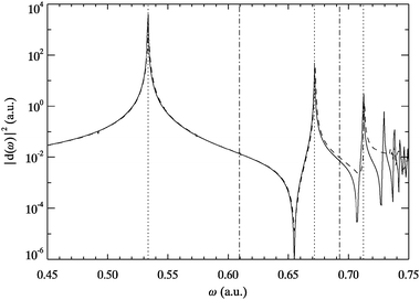

Fig. 1 Dipole power spectrum for helium obtained from TDSE (solid line) and AE-TDKSE (dashed line). Vertical lines indicate the first five transition energies from the ground state to singlet states of odd (dotted) and even parity (dotted-dashed) as obtained from eqn (2.3).

Fig. 2 Quadrupole power spectrum for helium obtained from TDSE (solid line) and AE-TDKSE (dashed line). Vertical lines indicate the first five transition energies from the ground state to singlet states of odd (dotted) and even parity (dotted-dashed) as obtained from eqn (2.3).

In trying to understand the excellent performance of the AE approximation we now investigate the nature of the observed excitations. To this end we project the correlated final states ψ_f on symmetric KS product wave functions

constructed from the exact occupied and unoccupied orbitals of eqn (2.8) for helium. In this way we can estimate the single and double excitation character of a correlated excited state with respect to the KS basis. Table 2 shows the overlap between the KS product states and the first six eigenstates of the helium Hamiltonian of eqn (2.2). States 1 to 5 are the final states of the transitions denoted with vertical lines in Fig. 1 and 2. Clearly they are completely dominated by states Φ_ij with single excitation character. This fits in with the general concept of energy levels in the helium atom where the single particle picture is known to work well.

Table 2 Projection amplitudes |〈Φ_ij|ψ_f〉|² of correlated singlet states ψ_f on KS product wave functions Φ_ij for the helium atom. Values less then 0.01 have been omitted

ij	f
	0	1	2	3	4	5
00	0.99
01		0.92		0.02
02			0.97
03		0.03		0.90		0.03
04					0.93
05				0.05		0.82
06					0.04
07						0.09
09						0.01
12		0.02

---

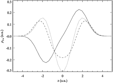
The transition densities for helium are shown in Fig. 3. They can be interpreted as a momentary picture of the density redistribution during a transition: negative regions correspond to density removal while positive values signal density accumulation.^42,43 As a consequence of symmetry, the transition density is always antisymmetric for dipole and symmetric for quadrupole excitations. For helium we find for the dipole transitions a purely left–right oscillation (sloshing mode) and for quadrupole transitions an inward–outward redistribution (breathing mode) of decreasing intensity for growing energy. These patterns provide a hydrodynamic interpretation of the electron motion during a transition.

Fig. 3 Exact transition densities ρ_0n of helium excitations for n = 1 (solid), 2 (dotted), 3 (dashed) 4 (dotted-dashed) and 5 (triple-dotted-dashed).

The discussion so far and the excellent performance of the AE approximation begs the natural question: Where are the double excitations that are expected to be missed by the adiabatically exact approximation? Unfortunately (for our analysis), for the 1D helium atom they only appear above the first ionization threshold.^28,44 The lowest double excitations are in fact embedded in the one particle ionization continuum and thus have the character of autoionizing or Fano resonances.^45,46 They can only be expected at energies around 1.3 a.u.²⁸ which is far beyond the numerical accuracy of our AE-TDKSE scheme. Even if this regime could be reached, the peculiar degeneracy of a single and a double excitation which is characteristic of a Fano resonance would very likely complicate the analysis. Thus, we will now consider systems where the double excitations lie in the energy regime that can be resolved by the AE-TDKSE scheme.

To develop an intuition for what kind of systems one needs to study in order to find low-lying double-excitations, it is helpful to look at the problem from the KS perspective of independent particles. Due to the Coulombic asymptotics of the KS potential the single particle energy level spacing is quickly decreasing for growing energies (Rydberg series). This means that infinitely many single particle transitions are found at energies lower than one of the first double excitation. In order to circumvent this situation one needs a system with a more constant spacing of the energy levels. This requirement takes us to another typical 1D singlet system, namely Hooke’s atom. Here the intuitive argument based on the KS transitions implies that the excitation of two electrons to the first excited state (i.e., a double excitation) will be roughly in the energy range of the transition of one electron to the second excited state (one of the lower single excitations).³⁶ As the energy spectrum of the harmonic external potential is completely discrete there is also no issue with Fano-type degeneracies.

B Hooke’s atom

The dipole response of Hooke’s atom is shown in Fig. 4. For this systems we found the AE-TDKSE results to be converged for ω < 1 a.u. Here the power spectrum is more irregular with respect to the order of positive and negative parity than for helium. Clearly the dominant transition for dipole excitations is at the harmonic frequency ω₀₁ = (k/m)^½, which is well reproduced by the AE-TDKSE results. This agreement is a consequence of the fact that to first order linear response the dipole boost resembles an applied time-dependent dipole field. Thus the response to the latter in Hooke’s atom is exactly reproduced by the adiabatically exact approximation due to the applicability of the harmonic potential theorem.^27,47 The dominance of the harmonic frequency leads to suppression of higher dipole active transitions like f = 4,5 in agreement with almost vanishing oscillator strengths of these excitations.⁴⁸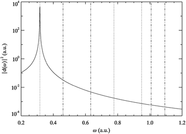

Fig. 4 Dipole power spectrum for Hooke’s atom obtained from TDSE (solid line) and AE-TDKSE (dashed line directly on top). Vertical lines indicate transition energies of the ground state to singlet states of odd (dotted) and even parity (dotted-dashed).

The quadrupole power spectrum (cf.eqn (2.14)) shown in Fig. 5 reveals that instead of the excitations f = 2,3 there is only one transition at ω≈ 0.5 a.u. in the AE approximation. Apparently we have finally encountered a situation where the adiabatically exact approximation does not yield the proper excitation frequency.

Fig. 5 Quadrupole power spectrum for Hooke’s atom obtained from TDSE (solid line) and AE-TDKSE (dashed line). Vertical lines indicate transition energies of the ground state to singlet states of odd (dotted) and even parity (dotted-dashed).

Consequently, we investigate once more the single particle character of the relevant excitations. The projections of the final states on the Hooke KS basis are shown in Table 3. We find that, in contrast to the helium atom, even the lower states have nonvanishing double excitation contributions. The transition f = 1, though, is still predominantly of single excitation character in agreement with the ability of the AE-TDKSE to reproduce the corresponding peak in the spectrum. For f = 2, 3 there is already a strong contribution of the Φ₁₁ product state which can explain the failure of the AE-TDKSE in this energy regime.

Table 3 Projection amplitudes |〈Φ_ij|ψ_f〉|² of correlated singlet states ψ_f on KS product wave functions Φ_ij for Hooke. Values less then 0.01 have been omitted

ij	f
	0	1	2	3	4	5	6
00	0.92		0.02	0.03
01		0.81			0.10	0.05
02			0.54	0.35
03		0.03			0.72	0.18
04				0.05			0.13
05						0.05
11	0.07		0.43	0.40
12		0.14			0.16	0.54
13				0.02			0.49
14		0.01			0.02
22				0.14			0.36
23						0.16

---

To obtain a better understanding of the relevant excitations we once more look at the transition densities. For the first six excitations they are shown in Fig. 6 and 7. We find sloshing (f = 1) and breathing (f = 2) type excitations as in the helium atom but also higher order transitions (f = 3–6) that no longer show a structure which can easily be related to one of these two types.

Fig. 6 Exact transition densities ρ_0n of Hooke excitations for n = 1 (solid), 2 (dotted) and 3 (dashed).

Fig. 7 Exact transition densities ρ_0n of Hooke excitations for n = 4 (solid), 5 (dotted) and 6 (dashed).

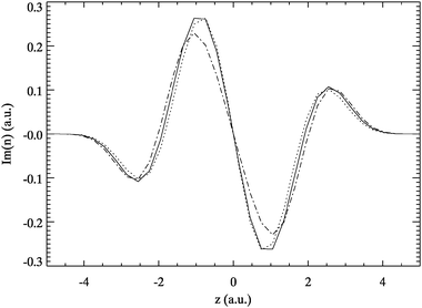
The transition densities can further be used to sort out which excitation is reproduced by the AE approximation and which is not. Based on the structure of the transition density, one can identify which exact transition belongs to which (shifted) AE peak. The adiabatically exact transition densities obtained from the Fourier transform of the time-dependent density (see above) provide some evidence that the peak at ω≈ 0.5 a.u. should correspond to the f = 2 excitation: as shown in Fig. 8 the structure of the first two transitions present in the AE spectrum closely resembles that of the exact excitations f = 1,2. This means that the second transition is properly reproduced by the AE-TDKSE with respect to its breathing-type character but it is shifted to the wrong energy. At the same time the f = 3 excitation is missed completely by the AE approximation. So despite the fact that in view of table 3 both the f = 2 and the f = 3 transitions could be termed “double excitations” the AE approximation treats them quite differently.

Fig. 8 Adiabatically exact transition densities of Hooke obtained from the Fourier transform of the time-dependent AE-TDKSE density (see text). The shown transition densities correspond to the adiabatically exact transitions found at ω≈ 0.32 (solid) and 0.50 a.u. (dotted), cf.Fig. 4 and 5. All curves were scaled so that the peak heights are roughly the same to allow for better comparison with the exact transition densities of Fig. 6.

C Anharmonic Hooke’s atom

To obtain a more complex structure of the dipole response we finally turn to the anharmonic version of Hooke’s atom. The dipole power spectrum of A6-Hooke shown in Fig. 9 indicates that the first transition is well reproduced but the AE-TDKSE produces only one peak at ω≈ 1.3 a.u. instead of the f = 4 and f = 5 excitations. These energies are still well within the numerical validity regime of the AE-TDKSE which extends up to ω≈ 1.8 a.u. From the quadrupole power spectrum in Fig. 10 we can infer that the AE approximation produces a peak at ω≈ 0.77 a.u. instead of the f = 2 and 3 peaks. By varying the boost parameter we found the peaks at ω≈ 0.88 and 1.74 a.u. to be higher order effects that can be neglected in our discussion of the linear response regime. The excitations to f = 6,7 are not present in the AE spectrum. One may speculate that the AE-TDKSE scheme might still be approximately valid around ω≈ 2 a.u. and that thus the AE approximation reproduces only one peak (ω≈ 1.9 a.u.) in the range of the f = 6,7,8 quadrupole triple. This would correspond to the AE-TDKSE producing only one peak among the quadrupole double f = 2,3 and the dipole double f = 4,5 respectively. In any case we have encountered two more situations where peaks are shifted to wrong energies or missing completely from the AE spectrum.

Fig. 9 Dipole power spectrum for A6-Hooke obtained from TDSE (solid line) and AE-TDKSE (dashed line). Vertical lines indicate transition energies of the ground state to singlet states of odd (dotted) and even parity (dotted-dashed).

Fig. 10 Quadrupole power spectrum for A6-Hooke obtained from TDSE (solid line) and AE-TDKSE (dashed line). Vertical lines indicate transition energies of the ground state to singlet states of odd (dotted) and even parity (dotted-dashed).

The projections for A6-Hooke are shown in Table 4. Again, a strong double excitation character is present for f > 1. One may wonder whether this difficulty is generally just a consequence of the chosen basis set. To check this we also used the single particle states corresponding to the v_ext,0 of A6-Hooke as a basis (instead of the KS orbitals) and performed the overlap analysis once more. This leads to numbers quite similar to the ones reported in Table 4.

Table 4 Projection amplitudes |〈Φ_ij|ψ_f〉|² of correlated singlet states ψ_f on KS product wave functions Φ_ij for A6-Hooke. Values less then 0.01 have been omitted

ij	f
	0	1	2	3	4	5	6	7
00	0.95		0.03	0.02
01		0.91			0.07
02			0.31	0.63				0.03
03					0.36	0.61
04								0.30
11	0.04		0.66	0.26				0.03
12		0.08			0.56	0.31
13				0.02			0.32	0.43
14
22				0.06			0.66	0.18
23						0.05
33								0.02

---

Once more the success for the f = 1 transition seems to be a consequence of the predominant single excitation character of ψ₁. The failure for f > 1 is again a consequence of considerable double excitation contribtion. It appears especially plausible that f = 6 is missing as ψ₆ is exclusively of double excitation character.

The transition densities for A6-Hooke are shown in Fig. 11 to 12. Similar to Hooke’s atom we only find exclusive sloshing and breathing signatures for the lowest transitions. The higher excitations show a variety of patterns.

Fig. 11 Exact transition densities ρ_0n of A6-Hooke excitations for n = 1 (solid), 2 (dotted) and 3 (dashed).

Fig. 12 Exact transition densities ρ_0n of A6-Hooke excitations for n = 4 (solid), 5 (dotted), 6 (dashed) and 7 (dotted-dashed).

For sorting out which AE excitation corresponds to which exact one the transition densities are again a helpful tool. Comparing the AE transition density at ω≈ 0.77 to the ones for f = 2 and 3 in Fig. 13 shows that the AE excitation rather resembles f = 2. This implies that the latter transition is shifted to the wrong excitation energy while f = 3 is completely absent. This is noteworthy because ψ₃ has a smaller double excitation contribution than ψ₂. A similar situation is found for f = 4,5 as shown in Fig. 14.

Fig. 13 AE transition density of A6-Hooke at ω≈ 0.77 a.u. (solid) and the exact ρ_0f for f = 2 (dotted) and 3 (dotted-dashed). All curves were scaled to allow for better comparison.

Fig. 14 AE transition density of A6-Hooke at ω≈ 1.3 a.u. (solid) and the exact ρ_0f for f = 4 (dotted) and 5 (dotted-dashed). All curves were scaled to allow for better comparison.

IV. Summary and outlook

We have explored the performance of the adiabatically exact approximation—i.e., no temporal nonlocality but full spatial nonlocality—for the linear response of 2-electron systems. It is known that this approximation is not able to generally provide the exact excitation energies. This property follows from the Casida equation in a formal way but one is only beginning to understand its practical consequences for the adiabatically exact spectrum.¹² In the present article we examine this relation more closely.

So far, it has commonly been assumed that adiabatic approximations are missing the transitions of double excitation character, or at least shift them to wrong energies. On the other hand they are expected to work for single excitations. We found that this concept generally applies to the AE approximation, but that the situation is involved when double excitations are present.

For the lower discrete part of the spectrum of the helium atom the transitions are of genuinely single excitation character and hence the AE-TDKSE reproduces all peaks of the exact spectrum. It even locates them at the virtually exact energies. These findings imply that the xc kernel in this energy regime is well represented by its ω→ 0 limiting case, i.e., the ground state kernel. This situation is a consequence of the special nature of the system. Here double excitations are to be expected only above the first ionization threshold where they take the form of autoionizing resonances embedded in the one particle continuum.

The situation is different in the Hooke-type systems that we studied. Here large parts of the spectrum are incorrectly predicted by the AE approximation, i.e., peaks are shifted to wrong energies or missed completely. Already at the lower energies the double excitation character of a given transition is non-negligible. However, it is not straightforward to relate the failures for a specific transition to the corresponding magnitude of the double excitation contribution. Apparently it is not enough to consider the single particle character of an excitation to infer whether it will be missed or just shifted by the AE approximation.

We found transition densities to be a suitable tool to get deeper insight into the structure of specific excitations. Although they also do not provide a clear criterion to identify particularly nonadiabatic transitions, they allow for a better comparison of certain transitions and facilitate matching of exact transitions to peaks that are incorrectly shifted in the AE spectrum.

Finally, the transition densities provide a route to a more intuitive hydrodynamic view of electronic excitations. Such a hydrodynamical perspective may be a new way to obtain an understanding of nonadiabatic effects.^27,49

Acknowledgement

We acknowledge financial support by the Deutsche Forschungsgemeinschaft.

References

1. J. F. Dobson and B. P. Dinte, Phys. Rev. Lett., 1996, 76, 1780.
2. G. F. Bertsch, J.-I. Iwata, A. Rubio and K. Yabana, Phys. Rev. B, 2000, 62, 7998.
3. I. V. Tokatly and O. Pankratov, Phys. Rev. Lett., 2001, 86, 2078.
4. G. Onida, L. Reining and A. Rubio, Rev. Mod. Phys., 2002, 74, 601.
5. J. R. Chelikowsky, L. Kronik and I. Vasiliev, J. Phys.: Condens. Matter, 2003, 15, R1517.
6. D. Rappoport and F. Furche, J. Am. Chem. Soc., 2004, 126, 1277.
7. A. Zangwill and P. Soven, Phys. Rev. A, 1980, 21, 1561.
8. E. Runge and E. K. U. Gross, Phys. Rev. Lett., 1984, 52, 997.
9. M. Petersilka, U. Gossmann and E. K. U. Gross, Phys. Rev. Lett., 1996, 76, 1212.
10. E. K. U. Gross, J. F. Dobson and M. Petersilka, in Density Functional Theory, ed. R. F. Nalewajski, Springer, Berlin, 1996, pp. 81–172.
11. M. E. Casida, in Recent Advances in Density Functional Methods, Part I, ed. D. P. Chong, World Scientific Publishing, Singapore, 1995, pp. 155–192.
12. N. T. Maitra, F. Zhang, R. J. Cave and K. Burke, J. Chem. Phys., 2004, 120, 5932.
13. S. Hirata and M. Head-Gordon, Chem. Phys. Lett., 1999, 302, 375.
14. D. J. Tozer and N. C. Handy, Phys. Chem. Chem. Phys., 2000, 2, 2117.
15. R. J. Cave, F. Zhang, N. T. Maitra and K. Burke, Chem. Phys. Lett., 2004, 389, 39.
16. J. Neugebauer, E. J. Baerends and M. Nooijen, J. Chem. Phys., 2004, 121, 6155.
17. K. J. H. Giesbertz, E. J. Baerends and O. V. Gritsenko, Phys. Rev. Lett., 2008, 101, 033004.
18. K. Yabana and G. F. Bertsch, Phys. Rev. B, 1996, 54, 4484.
19. U. Saalmann and R. Schmidt, Z. Phys. D, 1996, 38, 153.
20. F. Calvayrac, P. G. Reinhard and E. Suraud, Ann. Phys. (N.Y.), 1997, 255, 125.
21. M. Marques, A. Castro, G. Bertsch and A. Rubio, Comput. Phys. Commun., 2003, 151, 60.
22. M. Mundt and S. Kümmel, Phys. Rev. B, 2007, 76, 035413.
23. H. Appel, E. K. U. Gross and K. Burke, Phys. Rev. Lett., 2003, 90, 043005.
24. M. Thiele, E. K. U. Gross and S. Kümmel, Phys. Rev. Lett., 2008, 100, 153004.
25. I. D’Amico and G. Vignale, Phys. Rev. B, 1999, 59, 7876.
26. P. Hessler, N. T. Maitra and K. Burke, J. Chem. Phys., 2002, 117, 72.
27. M. Thiele and S. Kümmel, Phys. Rev. A, 2009 , submitted.
28. S. L. Haan, R. Grobe and J. H. Eberly, Phys. Rev. A, 1994, 50, 378.
29. D. G. Lappas, A. Sanpera, J. B. Watson, K. Burnett, P. L. Knight, R. Grobe and J. H. Eberly, J. Phys. B, 1996, 29, L619.
30. D. Bauer, Phys. Rev. A, 1997, 56, 3028.
31. S. L. Haan and R. Grobe, Laser Phys., 1998, 8, 885.
32. D. G. Lappas and R. van Leeuwen, J. Phys. B, 1998, 31, L249.
33. W.-C. Liu, J. H. Eberly, S. L. Haan and R. Grobe, Phys. Rev. Lett., 1999, 83, 520.
34. M. Lein, E. K. U. Gross and V. Engel, Phys. Rev. Lett., 2000, 85, 4707.
35. R. Panfili and W.-C. Liu, Phys. Rev. A, 2003, 67, 043402.
36. E. Orestes, K. Capelle, A. B. F. da Silva and C. A. Ullrich, J. Chem. Phys., 2007, 127, 124101.
37. A. S. de Wijn, S. Kümmel and M. Lein, J. Comput. Phys., 2007, 226, 89.
38. P. Hohenberg and W. Kohn, Phys. Rev., 1964, 136, B864.
39. Time-dependent Density Functional Theory, ed. M. Marques, C. Ullrich, F. Nogueira, A. Rubio, K. Burke and E. Gross, Springer, Berlin, 2006.
40. M. Mundt, S. Kümmel, R. van Leeuwen and P.-G. Reinhard, Phys. Rev. A, 2007, 75, 050501.
41. R. A. Broglia, G. Coló, G. Onida and H. E. Roman, Solid State Physics of Finite Systems, Springer, Berlin, 2004.
42. S. Kümmel, K. Andrae and P.-G. Reinhard, Appl. Phys. B, 2001, 73, 293.
43. S. Tretiak and S. Mukamel, Chem. Rev., 2002, 102, 3171.
44. To the best of our knowledge this applies to all atomic systems.
45. U. Fano, Phys. Rev., 1961, 124, 1866.
46. H. Friedrich, Theoretical Atomic Physics, Springer, Heidelberg, 2006.
47. J. F. Dobson, Phys. Rev. Lett., 1994, 73, 2244.
48. The oscillator strengths 2|〈ψ₀|z|ψ_f〉|²ω_0f can be computed directly from the exact eigenstates.
49. C. A. Ullrich and K. Burke, J. Chem. Phys., 2004, 121, 28.

---