Powder NMR crystallography of thymol

Abstract

A protocol for the structure determination of powdered solids at natural abundance by NMR is presented and illustrated for the case of the small drug molecule thymol. The procedure uses proton spin-diffusion data from two-dimensional NMR experiments in combination with periodic DFT refinements incorporating ¹H and ¹³C NMR chemical shifts. For thymol, the method yields a crystal structure for the powdered sample, which differs by an atomic root-mean-square-deviation (all atoms except methyl group protons) of only 0.07 Å from the single crystal X-ray diffraction structure with DFT-optimized proton positions.

---

1. Introduction

Structural characterization of powdered samples is of ever increasing importance for a wide range of contemporary materials-related problems, including, for example, the characterization of inorganic framework materials¹ or of polymorphic pharmaceutical compounds.²

While X-ray diffraction remains the method of choice for structure determination of single crystals, three main approaches are used for crystallographic characterization of powders: powder X-ray (or neutron) diffraction,³ computationally based structure prediction techniques⁴ and solid-state NMR.

In this respect, the field of NMR crystallography has seen very rapid growth over the past few years. Impressive results have been shown for NMR structure determination in inorganic framework materials.^1,5 In the field of molecular crystals, there has been particular progress towards structure validation methods by developing approaches to assign natural abundance solid-state NMR spectra, and then combining this with state-of-the art DFT chemical shift calculation methods.^6,7 These validation methods allow also the assignment of a given powder form to a known crystal structure (usually obtained from single crystal X-ray diffraction). These approaches are particularly powerful, and have even been used to identify polymorphs in the presence of excipient mixtures in pharmaceutical tablet formulations.⁸

Moreover, we have recently introduced approaches that not only validate a structure but also offer the possibility of complete ab initio structure determination in molecular powders using combined NMR and computational methods. We have illustrated how proton spin-diffusion (PSD) curves can be analysed in terms of molecular conformation and crystal packing,⁹ and shown that PSD data can be incorporated as restraints in a molecular modelling based structure determination.¹⁰ The result of the molecular modelling step can then be used as the starting point for DFT refinement, to yield a final structure which can be validated using NMR chemical shifts. For the dipeptide β-L-Asp-Ala, we obtained a structure in this way that deviates from the known crystal structure by an all-atom root-mean-square-deviation (rmsd) of only 0.13 Å.¹¹

In this article we assemble these elements together for the first time to present a complete protocol for structure determination by NMR crystallography in molecular crystals. The method is applied to the molecule thymol. Thymol is a monoterpene found in oil of thyme and other spices. It has strong antiseptic properties, and is a synthetic precursor of menthol. It is appropriate in the present context, since due to the ease of obtaining large crystals it was among the first systems studied by crystallographers, even before the advent of X-ray methods.^12,13 By applying the protocol introduced here, we determine a structure for powdered microcrystalline thymol where the heavy atom positions are found to be identical to the single crystal X-ray diffraction structure.

2. Experimental

2a Sample

Powdered thymol was purchased from Acros Organics and recrystallized by slow evaporation of pentane. For the NMR study, the crystals were carefully ground to give a powder. The crystal structure of thymol (5-methyl-2-(1-methylethyl)phenol, CSD¹⁴ code entry: IPMEPL), was previously determined by Thozet and Perrin¹³ from single crystal X-ray diffraction data. The cell is rhombohedral (space group R3̄) and can be described using the primitive unit cell (6 symmetry equivalent molecules in the unit cell, a₀= b₀= c₀ = 11.476 Å, α = β = γ = 79.85°) or the hexagonal unit cell representation (18 molecules in the unit cell, a₀= b₀ = 14.730 Å, c₀ = 23.115 Å, α = β = 90°, γ = 120°).

2b X-Ray diffraction

An X-ray diffraction study was performed on a single crystal taken from the recrystallized sample in order to ensure that the structure was the same as that previously published.¹³ The single crystal structure determination was performed on a NONIUS Kappa CCD diffractometer. A powder X-ray diffraction spectrum from the sample ground for NMR was also recorded, on a Bruker D8 Advance diffractometer.

The structure of the single crystal was determined to be the same as that published and the powder diffraction pattern matches that calculated for the published structure.¹³

Note that, as is well known,¹⁵ X-ray diffraction is sensitive to the electronic charge density and hence generally less accurate in positioning (electron light) hydrogen atoms. Thus the proton positions in the structure obtained by single crystal X-ray diffraction were optimized using DFT with the parameters described in the experimental section, while keeping the heavy atom positions fixed. The resulting structure, called the reference structure here, was used to assess the overall performance of the method.

2c NMR experiments

NMR experiments were carried out at a nominal sample temperature of 293 K on a Bruker AVANCE III wide bore spectrometer operating at a ¹H Larmor frequency of 500.13 MHz, a Bruker AVANCE standard bore spectrometer operating at a ¹H Larmor frequency of 700.13 MHz, and a Bruker AVANCE III standard bore spectrometer operating at a ¹H Larmor frequency of 900.13 MHz. Experiments on the 500 and 700 MHz spectrometers were carried out with a Bruker 4 mm double resonance CPMAS probehead using a sample volume restricted to the central third of the rotor (PTFE inserts).

Proton chemical shifts were measured using a ¹H 1D spectrum acquired using a Bruker 1.3 mm double resonance CPMAS probehead at 900 MHz with a sample spinning frequency of 60 kHz and no homonuclear decoupling. This spectrum was referenced to the single resonance observed in adamantane for protons at 1.87 ppm with respect to neat TMS.

A 1D ¹³C CPMAS spectrum was recorded on the 500 MHz spectrometer at a sample spinning speed of 11 kHz for measuring ¹³C chemical shift. 128 transients were acquired with acquisition times of 30 ms, using a recycle delay of 3 s. A 5 ms CP contact time and a SPINAL-64¹⁶¹H RF field amplitude of 100 kHz were used. ¹³C chemical shifts were referenced with respect to the CH₂ resonance of adamantane at 38.48 ppm with respect to neat TMS.¹⁷

¹H high-resolution spectra were acquired using the eDUMBO-1₂₂¹⁸ homonuclear decoupling scheme in the indirect dimension and/or windowed DUMBO-1¹⁹ homonuclear decoupling during acquisition, using a decoupling cycle time of 32 μs and an RF field amplitude of 100 kHz.

The ¹H spectra shown in the figures have axes corrected for the homonuclear decoupling induced scaling factor, which is determined by fitting the peak positions obtained in homonuclear decoupled spectra to the well resolved peaks seen in the 60 kHz MAS-only spectrum. The methyl peaks were deconvoluted into three gaussian–lorentzian lineshapes using standard Bruker TOPSPIN software. The experimentally determined scaling factors were approximately 0.52 for w-DUMBO-1 and 0.58 for eDUMBO-1₂₂.

The 2D refocused ¹³C–¹³C INADEQUATE spectrum²⁰ was recorded on the 500 MHz spectrometer at a spinning speed of 12.5 kHz. A total of 100 t₁ points were acquired using States-TPPI²¹ with 640 scans each, with a maximum t₁ delay of 5.1 ms. Delays for the conversion to and from double-quantum coherence were 3.5 ms (synchronized with the rotor period). The CP contact time was 3.5 ms, and heteronuclear decoupling was achieved using SPINAL-64 with a ¹H RF field amplitude of 100 kHz. The recycle delay was 3.5 s. The total time for this experiment was 63 h.

The 2D refocused ¹H–¹³C INEPT spectrum²² was recorded at 500 MHz and a sample spinning frequency of 12.5 kHz. A total of 128 t₁ points were recorded using States-TPPI with 16 scans each, with a maximum t₁ delay of 6.1 ms. The evolution delays for the INEPT magnetization transfer were, respectively, 480 μs (creation of ¹H antiphase coherence) and 640 μs (refocusing of ¹³C antiphase coherence), synchronized with the rotor period. Heteronuclear decoupling was achieved with SPINAL-64 at a ¹H decoupling field amplitude of 100 kHz. The recycle delay was 4 s and the duration of this experiment was about 2 h.

The 2D ¹H–¹H double-quantum CRAMPS spectrum²³ was recorded on the 700 MHz spectrometer at a sample spinning speed of 6.6 kHz. A total of 256 t₁ points were acquired with 16 scans each using States-TPPI, with a maximum t₁ delay of 24.6 ms. The excitation and reconversion periods used 3 POST-C7²⁴ elements with a proton RF field amplitude of 46.2 kHz. The recycle delay was 3.5 s and the total duration of this experiment was 4 h.

2D ¹H–¹H spin-diffusion spectra were recorded at 700 MHz at a sample spinning rate of 6.6 kHz. 204 t₁ points were recorded with 16 scans each, with a maximum t₁ delay of 16.3 ms, using States-TPPI. Seventeen spectra with spin-diffusion delays τ_SD ranging from 0 to 2 ms were acquired in random order. The recycle delay was 3 s and each spectrum was acquired in about 3 h.

The experimental build-up curves were obtained by integration of the volumes of the cross-peaks for each spin-diffusion delay τ_SD. The signals of two isopropyl methyl groups, H(5–7) and H(8–10), are not resolved and their cross-peaks were thus integrated together.

2d PSD back-calculation and molecular modelling calculations

PSD (proton spin-diffusion) spectra were back-calculated from atomic coordinates and compared to experimental data using a home-written C++ routine described elsewhere^9,10 and adapted to the space group of thymol.

The difference between calculated and experimental build-up curves is evaluated in terms of the goodness-of-fit coefficient χ², calculated by the PSD back-calculation routine.

where calc_i and expt_i are the calculated and experimental cross-peak volumes and σ_i² is the noise on the data, taken as 1% of the methyl peak volume. The experimental noise is not the only source of error in the fit, as the model used for fitting is phenomenological, but no attempt has been made to quantify this error yet.

Molecular modelling was performed with the Xplor-NIH molecular modelling package,²⁵ as described previously.¹⁰

We used a standard molecular modelling force field including covalent terms (bond, angles, planarity) and van der Waals terms (both intra- and inter-molecular) to ensure a reasonable geometry.

The experimental NMR restraints were included by the definition of a PSD force field defined as

E_PSD = a_PSD×χ_PSD² (2)

where a_PSD = 104.5 kJ mol⁻¹ is the weight of this potential. This weight ensures that the agreement with the proton spin-diffusion experimental data will be the dominant term in the energy expansion during the molecular modelling optimization (about 15 times the energy due to the other potentials after optimization).

To determine the uncertainty on the values of χ², noise with a standard deviation equal to 1% of the volume of the most intense peak (methyl peak) was repeatedly added to the experimental volumes in the build-up curves, and the calculated build-up curves were refitted. The resulting probability distribution for χ² has a standard deviation of 0.55, that yields a 66% chance of getting the correct value in an interval of χ²±σ.

2e DFT Calculations

Geometry optimizations and chemical shift calculations were carried out using the DFT program CASTEP.²⁶ CASTEP uses a planewave basis set to describe the wavefunctions (it thus has an implicit translational symmetry) and is very well adapted to the description of solid crystalline systems. The GIPAW method,²⁷ used with ultrasoft pseudo-potentials,²⁸ provides an efficient method to calculate chemical shifts in crystalline solids.²⁹

The geometry optimizations were carried out using the PBE functional,³⁰ a cut-off energy of 610 eV, ultrasoft pseudo-potentials generated on the fly and a 2 × 2 × 2 Monkhorst–Pack k-point grid.³¹ These parameters were optimized for convergence of the quantity of interest.

Chemical shieldings σ_calc were calculated using the same parameters as those used for the geometry optimization. They were then converted to chemical shifts δ_calc using eqn (3):

δ_calc = σ_ref−σ_calc (3)

The reference shielding σ_ref was determined by fitting the chemical shieldings calculated for the reference structure to the experimental chemical shifts, keeping the slope fixed to −1. This value of σ_ref was used to convert all the calculated shieldings to the calculated chemical shifts. The chemical shieldings calculated for the methyl protons were averaged over the three protons to obtain a calculated shielding for each methyl group.

3. Protocol for powder NMR crystallography

Scheme 1 outlines the protocol for powder NMR crystallography used here. The first part of the protocol consists of the combination of the spin-diffusion restraints with molecular modelling to determine the crystalline structure.^9,10

Scheme 1 Flow chart for NMR crystallography.

In the second part, the resulting structures are refined using a DFT geometry optimization. Comparison between experimentally measured and calculated chemical shifts validates the final structures.¹¹

In the following sections we give the details of how each step is implemented, using thymol as an illustrative example.

4. NMR data analysis

The first step in the structure determination protocol is obtaining NMR data which will be used for restraining the molecular modelling structure determination and for the DFT refinement steps. The NMR data are used to assign spectra, provide PSD build-up curves and measure ¹H and ¹³C chemical shifts.

4a Assignment of the spectra and measurement of ¹H and ¹³C chemical shifts

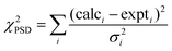
Four experiments are used to assign the ¹H and ¹³C resonances, as illustrated for thymol in Fig. 1. Site labels are shown in Fig. 1a. A 1D ¹³C CPMAS spectrum yields ¹³C chemical shifts. These are assigned with the help of a 2D ¹³C refocused INADEQUATE³² experiment, which yields the ¹³C assignment by giving connectivities between directly attached carbons. In the case of thymol this yields an unambiguous ¹³C assignment (if we assume that the C(1) carbon resonates at a lower field than the C(5) carbon), except for the C(8) and C(9) methyl groups which can be permuted. The 2D ¹H–¹³C refocused INEPT²² experiment is then used to correlate the resonances of the directly attached protons, thus providing the assignment for all the corresponding proton resonances except for the hydroxyl proton. The 2D ¹H–¹H double-quantum CRAMPS²³ experiment confirms the assignment, and identifies the hydroxyl proton present in the homonuclear decoupled proton spectra. The remaining uncertainty on the permutation of the C(8)H(5–7) and C(9)H(8–10) methyl groups does not hinder the proton spin-diffusion analysis as H(5–7) and H(8–10) cross-peaks are integrated together.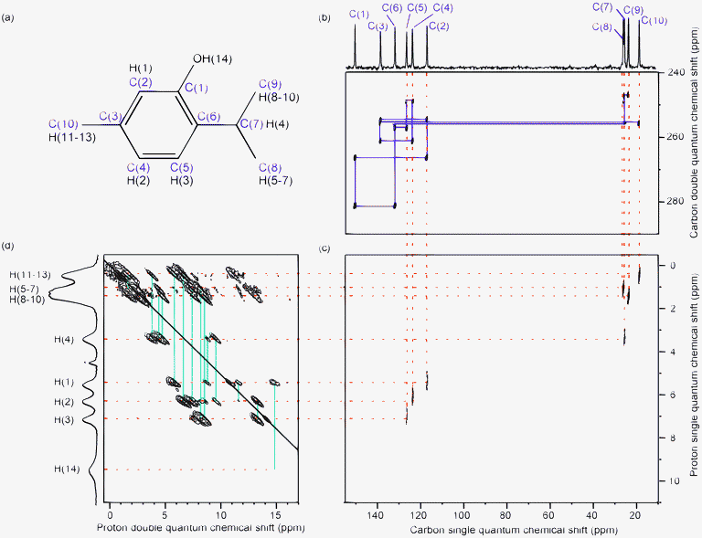

Fig. 1 Spectra used for assignment of ¹H and ¹³C chemical shifts: (a) structure and numbering of atoms in thymol, (b) 1D ¹³C CPMAS spectrum (top) and 2D ¹³C–¹³C refocused INADEQUATE spectrum (signals for the aliphatic region are folded, and the solid lines show the connection between covalently linked carbons), (c) 2D ¹H–¹³C INEPT spectrum and (d) ¹H–¹H double-quantum CRAMPS spectrum (the solid lines show the pairs of correlated signals) and ¹H homonuclear decoupled 1D spectrum. Dotted lines link the 1D ¹³C CPMAS spectrum shown above (b) to the 1D homonuclear decoupled ¹H projection shown to the side of (d) via the peaks in the 2D spectra. The asterisk indicates the carrier frequency artefact in the ¹H spectrum.

This is disentangled in the second part of the protocol (structure refinement), using ¹H chemical shift calculations. The ¹³C and ¹H chemical shifts thus determined are given in Table 1.

Table 1 Experimentally measured chemical shifts of thymol. Asterisks indicate values obtained by deconvolution. Labels are as in Fig. 1

Carbon label	^13C chemical shift (ppm)	Proton label	^1H chemical shift (ppm)
C(1)	150.2	H(1)	5.40
C(2)	116.9	H(2)	6.19
C(3)	138.4	H(3)	7.08
C(4)	123.6	H(4)	3.38
C(5)	126.3	H(5–7)	1.05*
C(6)	131.7	H(8–10)	1.45*
C(7)	25.5	H(11–13)	0.42*
C(8)	26.1	H(14)	9.99
C(9)	23.6	—	—
C(10)	18.7	—	—

---

4b Experimental ¹H–¹H spin-diffusion build-up curves

The pulse scheme shown in Fig. 2a was used to obtain a series of two-dimensional ¹H–¹H spin-diffusion correlation spectra. It should be noted that the feasibility of the entire method presented here for natural abundance samples depends on the resolution of the proton spectrum, and thus the performance of the dipolar decoupling schemes is central for success. It is therefore of particular importance that the experiments used here which involve homonuclear decoupling use the best possible schemes. In our hands, best results are obtained with the DUMBO family (eDUMBO-1¹⁸ during t₁ and the w-DUMBO-1¹⁹ for direct acquisition), though reasonable results can also be achieved with the PMLG³³ family of schemes.

Fig. 2 (a) Pulse sequence for the 2D ¹H–¹H spin-diffusion experiment. (b) 2D ¹H–¹H spin-diffusion spectrum of thymol for τ_SD = 1 ms. Boxes indicate the regions used for integration of each cross-peak. Asterisks indicate the carrier frequency artefacts.

Each peak in the 2D spectrum contains information about dipolar driven magnetization exchange (Fig. 2b). For example, the cross-peak in the top left corner of the spectra is the result of magnetization exchanged from the magnetically equivalent CH₃ protons evolving at the lowest chemical shift during t₁ to the OH protons evolving at the highest chemical shift during t₂. The dynamics of these magnetization exchanges can be followed by recording the evolution of the ¹H–¹H spin-diffusion spectrum when varying the spin-diffusion delay τ_SD. To this end the measured volume of each peak in the 2D spectrum is plotted as a function of the spin-diffusion delay τ_SD to obtain a series of build-up curves shown in Fig. 3.

Fig. 3 ¹H–¹H spin-diffusion build-up curves for thymol. Experimental data points are represented with blue circles; the best fit from the rate matrix analysis using the X-ray structure is shown using red lines.

4c Back-calculation of ¹H–¹H spin-diffusion build-up curves

Distance information cannot be extracted directly from these build-up curves, since each individual cross-peak contains contribution from tens of equivalent pairs of exchanging protons, corresponding to inter- and intramolecular interactions. Neither is it currently possible to calculate spin-diffusion curves from basic principles (spin-diffusion dynamics implies too many spins and too many interactions to be calculated accurately for a given crystal geometry).³⁴

To counter these problems, we have proposed using a phenomenological rate matrix description of the build-up curves. This has been shown to be surprisingly accurate.^9,10 Using this approach, predicted build-up curves can be calculated for any given trial crystal structure, using the home-made C++ routine.

The routine (illustrated in Scheme 2) uses the coordinates of a single molecule of the trial structure as input. Symmetry-related molecules are generated from the coordinates to build a full unit cell. Space group and unit cell parameters are taken from the powder X-ray diffraction data, as they are usually easily obtained from a powder diffractogram.^3,15 A larger part of the crystal is then generated by repeated translations of the full unit cell.

Scheme 2 Schematic routine for the use of ¹H–¹H spin-diffusion data.

The routine computes intra- and intermolecular distances r_ij between protons i and j in the trial crystal structure to simulate build-up curves P_ij according to eqn (4).

P_ij(τ_SD) = exp(−Kτ_SD)_ijM^j,0_z (4)

where M_z^j,0 is the volume of the diagonal peaks for τ_SD = 0 s and the elements of the K matrix are given by eqn (5,6).Each cross-peak build-up curve is thus in fact a sum of different curves arising from dipolar interaction with many different equivalent molecules. Full details of this approach have been published elsewhere.⁹

Note that here the rate of exchange k_ij between the protons within a given methyl group was increased by a factor of 100 to simulate a fast three site hopping motion in the calculation of the build-up curves.¹⁰ In the case of thymol, the two isopropyl methyl groups are not sufficiently resolved to be treated individually, so the rates of both methyl groups are summed in the following analysis.

Finally, the routine is used to fit the calculated build-up curves to the experimental ones by adjusting the only variable parameter, the phenomenological scaling factor A in eqn (5). The difference between calculated and experimental build-up curves is evaluated in terms of goodness-of-fit coefficient χ², as described in the experimental part.

Using this method, Fig. 3 shows a comparison between the experimental build-up curves and the calculated ones for the published single crystal X-ray diffraction determined structure. In this case χ² = 36.87.

The size of the crystal used in the calculation plays an important role in the accuracy of the result. Fig. 4a shows that pairs of spins distant from each other by up to 15 Å provide significant contributions to χ². This corresponds to generating about 60 molecules defining 10 646 distances between atom pairs to be included in the calculation (Fig. 4b). This illustrates clearly how the spin-diffusion data depend not only on the intramolecular distances (essential for determining the molecular confirmation) but also on the intermolecular distances, essential for determining the crystal packing.

Fig. 4 (a) Goodness-of-fit coefficient χ² as a function of the calculated crystal radius and (b) cluster corresponding to the 15 Å crystal radius.

5. Molecular modelling using PSD data

The second step in the structure determination is to use molecular modelling restrained by experimental PSD build-up curves to obtain an ensemble of potential thymol structures. Here, molecular modelling is performed using the Xplor-NIH package²⁵ with the experimental restraint implemented as the pseudo-energy term E_PSD defined in eqn (2), with a_PSD = 104.5 kJ mol⁻¹.

The general method used for the modelling stage of the determination of the crystal structure of thymol is shown in Scheme 3. First, 3000 starting structures with random atomic coordinates are generated. These structures are then subject to a high temperature (1500 K) molecular dynamics loop of 2000 steps of duration 0.005 ps followed by an annealing loop of 1000 steps of duration 0.003 ps, during which the van der Waals radius and forces are increased as the temperature is decreased. The 300 structures that are in best agreement with the spin-diffusion data are then selected (E_PSD < 6670 kJ mol⁻¹).

Scheme 3 Molecular modelling steps.

These 300 structures are then optimized using a combination of simplex³⁵ and Powell³⁶ minimizations, incorporating the experimental E_PSD term. Note that the simplex procedure is used when the spin-diffusion pseudo-energy term is employed, since we have not implemented the calculation of the derivative of the E_PSD term³⁷ with respect to the coordinates of all the atoms, and thus minimization routines using gradients cannot currently be used. In this cycle, a first simplex energy minimization is performed using the spin-diffusion pseudo-energy as the leading term, and with periodic van der Waals and geometrical potentials to ensure physically reasonable structures. The simplex method is known to be a poor minimization method that often locates local minima, but it has the advantages of not requiring gradients, and of being robust with respect to noise in the data. To speed up the process and escape from these local minima, a Powell optimization step follows, with only the geometrical and the periodic van der Waals potentials. This is then followed by a final simplex step with the same parameters as the first to further optimize with respect to the spin-diffusion pseudo-potential.

The 42 lowest energy structures (referred to as “PSD-optimized structures” in the following) were then selected, based solely on the best agreement with the experimental spin-diffusion data (E_PSD < 2925 kJ mol⁻¹). The 42 structures cover a spread in χ² of 1.1, which is estimated roughly to be the uncertainty in the determination as described in the experimental section 2.

Fig. 5 shows that the total energy of the optimized ensemble is indeed dominated by the spin-diffusion pseudo-energy term but that the geometrical and van der Waals terms are not directly correlated with the spin-diffusion data. Importantly, this illustrates that the structures could not be determined by modelling alone with the same Xplor-NIH energy terms.

Fig. 5 Xplor-NIH total energy (red circles) and PSD energy (blue triangles) for the set of the 300 relaxed structures. The 42 lowest PSD-energy structures were selected (i.e. those with PSD energy less than 2925 kJ mol⁻¹)

The result of this modelling procedure is an ensemble of 42 “PSD-optimized” crystal structures with an all-atom standard deviation in coordinates within the ensemble of 0.25 Å. The all-atom rmsd is 0.32 Å between the average structure of the ensemble and the reference single crystal X-ray diffraction determined structure.

6. Periodic DFT geometry optimization and chemical shift calculation

To improve the PSD-optimized crystal structures, DFT calculations are performed using the planewave DFT program CASTEP²⁶ on a subset of molecules chosen from the 42 structures obtained after molecular modelling to be representative of the ensemble (the standard deviation of this ensemble is the same as the whole ensemble). CASTEP is used both to optimize the crystal geometry and to calculate chemical shifts used to validate the structure obtained.

6a Geometry optimization

Fig. 6 shows the 9 structures (referred to as a to i in the following) chosen to be representative of the ensemble. A further DFT geometry optimization was performed on each of those (it was neither practical nor it is necessary to optimize all the 42 structures). The 9 optimized structures shown in Fig. 6b are in better agreement with the reference structure (shown in orange) and the deviations among the structures are smaller than before DFT geometry optimization.

Fig. 6 (a) Nine structures from the PSD-optimized ensemble and (b) the same 9 structures after periodic DFT optimization. The orange structure is the reference structure.

Fig. 7a shows the changes in the atomic rmsd between the reference structure and each of the 9 structures before and after geometry optimization. The atomic rmsds are calculated for all atoms except for all the methyl protons. The methyl group protons are ignored since they are thought to have little physical meaning (the methyl group is in rapid rotation at room temperature). Since the orientation of the methyl group is clearly different between the reference structure and the optimized ensemble, it would lead to an artificially high value of the atomic rmsd.

Fig. 7 (a) Atomic root-mean-square-deviation (rmsd) of the PSD-optimized structures on the left (red) and the DFT-optimized structures on the right (blue) from the reference structure, excluding the methyl group protons and (b) atomic rmsd of the DFT-optimized structures on the left (blue) from the reference structure, excluding the methyl group protons and energies on the right (orange, arbitrary reference) calculated by CASTEP after geometry optimization. The energy of the reference structure is displayed on the right for comparison.

One of the notable features in the 42 PSD-optimized structures is the variety of O–H orientations present. The optimization leads to two groups of structures visible in Fig. 6b, in which the orientation of the hydroxyl proton is either nearly parallel to the plane of the aromatic ring and similar to the single crystal X-ray determined structure (structures a–f) or where the OH proton points out of the plane (structures g–i). This can also be seen clearly in Fig. 7b, where the rmsd between the reference structure and structures g–i is high and is correlated with a high calculated energy. For the structures a–f, these quantities are smaller. This difference is related to the orientation of the hydroxyl proton and will be discussed further in section 7 below.

6b Chemical shift calculations and structure validation

The agreement between calculated and experimental chemical shifts for a proposed structure can be used to validate that structure, and the improvement of the quality of the proposed structure can be confirmed by an enhancement of this agreement, without the need for a reference structure.

The uncertainty on the assignment of the methyl groups C(8)H(5–7) and C(9)H(8–10) has to be resolved at this step. Towards this end, the reference structure is used to calculate chemical shifts.⁷ The assignment is deduced from the best agreement between calculated and experimental chemical shifts. H(8–10) is determined to have a higher chemical shift than H(5–7), which implies, using the INEPT spectrum in Fig. 1, that C(9) has a lower chemical shift than C(8). Note that the same assignment is obtained from all the final DFT optimized structures.

Fig. 8 shows the difference between calculated and experimental chemical shifts for the 9 PSD-optimized structures and for the final DFT-optimized structures. The clear reduction of this difference after geometry optimization confirms a definite improvement of the structure. The scatter of the calculated chemical shifts is also greater before the DFT geometry optimization than after, with the final optimized structures being more similar to each other (as could already be seen in Fig. 6 and 7). However, two different groups of DFT-optimized structures, structures a–f and g–i, emerge from Fig. 8, when focusing on the hydroxyl proton H(14) chemical shift.

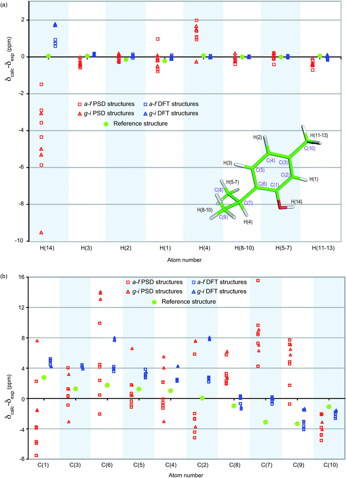Fig. 8 (a) ¹H and (b) ¹³C comparisons between calculated and experimental chemical shifts, displayed as the difference between calculated and experimental chemical shifts for each resonance. Red (left) corresponds to the structures before the DFT-optimization and blue (right) after optimization. Squares and triangles indicate structures where the orientation of the hydroxyl proton H(14) is respectively similar to (structures a–f) or different from (structures g–i) the reference structure (represented by green circles), respectively. Atoms appear in the same order as in the NMR spectra.

Table 2 shows the root-mean-square differences between the experimental chemical shifts for ¹H and ¹³C and the calculated chemical shifts for the reference structure. The PSD-optimized ensemble resulting from the first stage of the structure determination contains deviations in the atom positions that are corrected for by the DFT geometry optimization. On this basis, structures g–i are now rejected as their rms chemical shift difference with experimental ¹H chemical shifts is twice that for the a–f group. This again confirms the ability of chemical shifts to validate the final structures. Here even without knowledge of the crystal structure, this procedure selects the same O–H orientation as for the single crystal X-ray diffraction structure.

Table 2 Root-mean-square difference between experimental chemical shifts and calculated chemical shifts for the starting ensemble of the refinement step and for the final structures

	Rms difference between experimental and calculated ^1H chemical shifts (ppm)		Rms difference between experimental and calculated ^13C chemical shifts (ppm)
Name of structure	PSD	Final	PSD	Final
a	1.60	0.27	4.6	3.2
b	1.12	0.26	3.8	3.0
c	2.15	0.33	3.9	2.9
d	1.37	0.27	3.6	3.1
e	1.01	0.22	6.8	3.3
f	3.43	0.27	4.6	3.2
g	1.82	0.61	6.0	4.4
h	1.86	0.63	6.2	4.4
i	1.90	0.60	7.2	4.5
Reference	—	0.1	—	1.9

---

The final ensemble of acceptable structures (a–f) obtained by the combination of high-resolution ¹H and ¹³C NMR, ¹H spin-diffusion curves and DFT calculations is thus validated by the comparison of experimental and calculated chemical shifts. Their average coordinates form a structure that only differs from the reference structure by a rmsd of 0.07 Å (excluding methyl group hydrogens). This difference is less than the uncertainty in the positions in the reference structure itself. The two structures can thus be considered as identical.

7. Discussion

7a Hydrogen bonding in the crystal

As seen in Fig. 6b, two main hydroxyl-group orientations are observed in the PSD-optimized and the subsequent DFT-optimized structures. These orientations are related to hydrogen bonding in the thymol crystal. Fig. 9a shows the hydrogen bonding observed in the NMR determined structure, in agreement with the reference structure of thymol. The molecules form hexamers linked by hydrogen bonding interactions. Fig. 9b shows another potential arrangement of the molecules in the crystal, where the O–H⋯O bonds have a clockwise orientation, instead of the anticlockwise orientation for the X-ray structure. This configuration corresponds to the structures g–i determined above. A similar effect has already been seen in other molecular crystals.³⁸ If two single molecules from each of the two crystal configurations are compared, the O–H bond is apparently rotated by about 100° from one configuration to the other, as seen in Fig. 6b. However, in reality, the proton is simply displaced by about 1 Å in the direction of the oxygen in the neighbouring molecule, changing an O–H⋯O hydrogen bond into an O⋯H–O hydrogen bond. These two types of structure are thus very similar and it is not surprising that both appear as possibilities in the PSD-optimized ensemble and in the refined structures of Fig. 6. What is in fact remarkable here is that the protocol can reliably discriminate between them.

Fig. 9 Hexamers linked by hydrogen bonding in thymol for (a) the reference structure anticlockwise configuration and (b) the clockwise H-bonding configuration. The crystal is observed along the (111) axis of the rhombohedral cell.

7a(i) Proton spin-diffusion curves. As expected, the proton spin-diffusion build-up curves are sensitive to proton–proton distances. As the distances between protons in these two types of packing are very similar, excepting only the hydroxyl proton, the predicted build-up curves are quite similar for the two cases. This can be verified by studying the dependence of the predicted proton spin-diffusion curves on the rotation of the O–H bond about the C–O axis of the molecules in the whole crystal.

Fig. 10 shows the variation of χ², i.e. the goodness-of-fit coefficient, as a function of the dihedral angle θ C(2)–C(1)–O–H(14) for the PSD-optimized structure a. The configuration that gives the global minimum for a dihedral angle of −2° corresponds to the anticlockwise configuration of the reference structure (Fig. 9a), to within a difference of 16°. The second minimum at 91° is close to the DFT optimized clockwise configuration (dihedral angle value of 118°, shown in Fig. 9b). The difference in χ² (0.2) is too small to be significant and thus allows both hydrogen-bonding orientations as structural possibilities.

Fig. 10 Variation of the goodness-of-fit coefficient χ² when rotating the hydroxyl proton around the C–O axis on the PSD-optimized structure a, all other atoms fixed. The global minimum corresponds to hydrogen bonding as in Fig. 9a whereas the local minimum corresponds to hydrogen bonding as in Fig. 9b.

7a(ii) Periodic DFT energy and chemical shifts. Periodic DFT calculations are also sensitive to the H-bonding orientation of thymol. In Fig. 7b, the relative energies of “clockwise” structures g–i are higher than those of the “anticlockwise” structures, indicating, again, a preference for the reference configuration.

Another point of interest is that the orientation of the hydroxyl proton in structures g–i does not change to the anticlockwise orientation during the CASTEP geometry optimization. The fact that the optimization was not able to move the proton to the lowest energy position for structures g–i highlights the current need for very good PSD-optimized starting structures spanning all the reasonable possibilities for the DFT refinement step.

Finally, Fig. 8a shows that chemical shifts are also sensitive to hydroxyl orientation. Here, calculated chemical shifts of the hydroxyl proton H(14) for the optimized structures (blue, right) can be separated in two groups. Clockwise structures represented by triangles (structures g–i) have a significantly larger deviation in chemical shift from the experimentally measured values, with all the other anticlockwise structures (a–f) being in significantly better agreement with the experimental value.

In summary, all the techniques used here show the possibility of a structure presenting a different hydrogen bonding network, but we are able to identify the correct (anticlockwise) structure on the basis of the NMR observables.

7b Sensitivity to unit cell parameters

Finally, the sensitivity of proton spin-diffusion data to the packing of the molecules was tested. Structure a was chosen from the final DFT-optimized ensemble to test possibilities to restrain a series of deformations of the unit cell, illustrated in Fig. 11.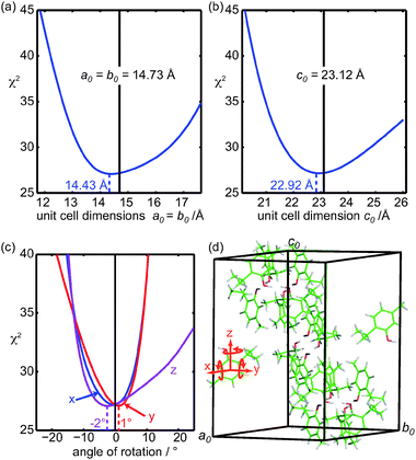

Fig. 11 Sensitivity of the PSD data to (a) and (b) the unit cell parameters, (c) orientation of the molecules in the unit cell on the PSD-optimized structure a, and (d) representation of the hexagonal unit cell parameters and the axes used for the rotations. The central lines in (a) and (b) indicate the X-ray determined unit cell parameters.

The unit cell dimensions a₀ and b₀ are equal in the space group R3̄ and were changed simultaneously. In this process, the unit cell was stretched but the molecules were not, leading to changes in the intermolecular distances but not the intramolecular ones. In Fig. 11a and 11b, the best agreement was found for unit cell parameters only 2% (for a₀ and b₀ cell dimensions) and 0.9% (for c₀) different from the single crystal X-ray diffraction determined values.

Furthermore, to highlight that the proton spin-diffusion data contain information on the orientation of the molecules in the unit cell, in Fig. 11c, the molecule used to generate the full crystal was rotated around three orthogonal axes x, y and z (Fig. 11d) before generation of the crystal. The variation of the goodness-of-fit coefficient is quite steep around the initial position, indicating that the orientation of the molecules in the unit cell is well defined.

8. Conclusion

We have presented a full procedure for natural abundance powder NMR crystallography, based on building blocks provided by previous work done in our laboratory^9–11 and we applied it to the example of powdered thymol. In this case the complete crystal structure is determined using high-resolution ¹H and ¹³C NMR data, and is found to be in perfect agreement with the previously known crystal structure.

Currently resolution in the proton spectrum is the limiting factor to wider application of this method. The achievement of a better ¹H NMR resolution by improving the homonuclear decoupling sequences and using higher spinning speeds in the future should increase the range of powdered materials that are ammenable to this type of study. Indeed, we note that similar strategies using proton spin-diffusion where ¹³C and ¹⁵N isotropic enrichment is possible has also led to structure determination of single molecules (but not so far of crystalline networks) in small molecules³⁹ but also in proteins.⁴⁰

Here, the powder can be studied as is, without any modifiation and at natural abundance. This opens the route to structure determination of microcrystalline powdered compounds in particular when the powder under study is not suitable for other structure determination methods, or can undergo changes in polymorphs during sample preparation. It should be of widespread interest in many areas, and particularly in pharmaceutical chemistry.

Acknowledgements

This work was supported in part by the Agence Nationale de la Recherche (ANR Blanc 06-1 139312-PSD-NMR). CJP is supported by the EPSRC. Spectra were recorded at the Rhône-Alpes Large Scale Facility for NMR. The calculations were carried out using the facilities provided by the Pôle Scientifique de Modélisation Numérique de Lyon.

References

1. J. Dutour, N. Guillou, C. Huguenard, F. Taulelle, C. Mellot-Draznieks and G. Ferey, Solid State Sci., 2004, 6, 1059–1067; N. Hedin, R. Graf, S. C. Christiansen, C. Gervais, R. C. Hayward, J. Eckert and B. F. Chmelka, J. Am. Chem. Soc., 2004, 126, 9425–9432; D. H. Brouwer, R. J. Darton, R. E. Morris and M. H. Levitt, J. Am. Chem. Soc., 2005, 127, 10365–10370; C. Gervais, C. Coelho, T. Azais, J. Maquet, G. Laurent, F. Pourpoint, C. Bonhomme, P. Florian, B. Alonso, G. Guerrero, P. H. Mutin and F. Mauri, J. Magn. Reson., 2007, 187, 131–140; D. H. Brouwer, J. Am. Chem. Soc., 2008, 130, 6306–6307; C. A. Fyfe and J. S. J. Lee, J. Phys. Chem. C, 2008, 112, 500–513.
2. H. G. Brittain, J. Pharm. Sci., 2008, 97, 3611–3636; R. K. Harris, Analyst, 2006, 131, 351–373.
3. K. D. M. Harris, M. Tremayne and B. M. Kariuki, Angew. Chem., Int. Ed., 2001, 40, 1626–1651.
4. G. M. Day, A. V. Trask, W. D. S. Motherwell and W. Jones, Chem. Commun., 2006, 54–56; G. M. Day, W. D. S. Motherwell and W. Jones, Phys. Chem. Chem. Phys., 2007, 9, 1693–1704; A. J. C. Cabeza, G. M. Day, W. D. S. Motherwell and W. Jones, Cryst. Growth Des., 2007, 7, 100–107; G. D. Enright, V. V. Terskikh, D. H. Brouwer and J. A. Ripmeester, Cryst. Growth Des., 2007, 7, 1406–1410.
5. C. A. Fyfe, A. C. Diaz, H. Grondey, A. R. Lewis and H. Forster, J. Am. Chem. Soc., 2005, 127, 7543–7558; C. A. Fyfe and D. H. Brouwer, J. Am. Chem. Soc., 2006, 128, 11860–11871; F. Pourpoint, C. Gervais, L. Bonhomme-Coury, T. Azais, C. Coelho, F. Mauri, B. Alonso, F. Babonneau and C. Bonhomme, Appl. Magn. Reson., 2007, 32, 435–457; D. H. Brouwer and G. D. Enright, J. Am. Chem. Soc., 2008, 130, 3095–3105; D. H. Brouwer, J. Magn. Reson., 2008, 194, 136–146.
6. R. K. Harris, P. Y. Ghi, R. B. Hammond, C. Y. Ma and K. J. Roberts, Chem. Commun., 2003, 2834–2835; R. K. Harris, Solid State Sci., 2004, 6, 1025–1037; V. Brodski, R. Peschar, H. Schenk, A. Brinkmann, E. R. H. van Eck, A. P. M. Kentgens, B. Coussens and A. Braam, J. Phys. Chem. B, 2004, 108, 15069–15076; C. E. Hughes, S. Olejniczak, J. Helinski, W. Ciesielski, M. Repisky, O. C. Andronesi, M. J. Potrzebowski and M. Baldus, J. Phys. Chem. B, 2005, 109, 23175–23182; M. Schulz-Dobrick, T. Metzroth, H. W. Spiess, J. Gauss and I. Schnell, ChemPhysChem, 2005, 6, 315–327; R. K. Harris, S. A. Joyce, C. J. Pickard, S. Cadars and L. Emsley, Phys. Chem. Chem. Phys., 2006, 8, 137–143; L. M. Shao, J. R. Yates and J. J. Titman, J. Phys. Chem. A, 2007, 111, 13126–13132; E. M. Heider, J. K. Harper and D. M. Grant, Phys. Chem. Chem. Phys., 2007, 9, 6083–6097; S. Olejniczak, J. Mikua-Pacboczyk, C. E. Hughes and M. J. Potrzebowski, J. Phys. Chem. B, 2008, 112, 1586–1593.
7. N. Mifsud, B. Elena, C. J. Pickard, A. Lesage and L. Emsley, Phys. Chem. Chem. Phys., 2006, 8, 3418–3422.
8. J. M. Griffin, D. R. Martin and S. P. Brown, Angew. Chem., Int. Ed., 2007, 46, 8036–8038; H. Hamaed, J. M. Pawlowski, B. F. T. Cooper, R. Q. Fu, S. H. Eichhorn and R. W. Schurko, J. Am. Chem. Soc., 2008, 130, 11056–11065.
9. B. Elena and L. Emsley, J. Am. Chem. Soc., 2005, 127, 9140–9146.
10. B. Elena, G. Pintacuda, N. Mifsud and L. Emsley, J. Am. Chem. Soc., 2006, 128, 9555–9560.
11. C. J. Pickard, E. Salager, G. Pintacuda, B. Elena and L. Emsley, J. Am. Chem. Soc., 2007, 129, 8932–8933.
12. W. J. Pope, J. Chem. Soc., Trans., 1899, 75, 455–465.
13. A. Thozet and M. Perrin, Acta Crystallogr., Sect. B: Struct. Sci., 1980, 36, 1444–1447.
14. F. H. Allen, Acta Crystallogr., Sect. B: Struct. Sci., 2002, 58, 380–388.
15. C. Giacovazzo, H. L. Monaco, G. Artioli, D. Viterbo, G. Ferraris, G. Gilli, G. Zanotti and M. Catti, Fundamentals of Crystallography, Oxford University Press, New York, 2002.
16. B. M. Fung, A. K. Khitrin and K. Ermolaev, J. Magn. Reson., 2000, 142, 97–101.
17. C. R. Morcombe and K. W. Zilm, J. Magn. Reson., 2003, 162, 479–486.
18. B. Elena, G. de Paëpe and L. Emsley, Chem. Phys. Lett., 2004, 398, 532–538.
19. D. Sakellariou, A. Lesage, P. Hodgkinson and L. Emsley, Chem. Phys. Lett., 2000, 319, 253–260; A. Lesage, D. Sakellariou, S. Hediger, B. Elena, P. Charmont, S. Steuernagel and L. Emsley, J. Magn. Reson., 2003, 163, 105–113.
20. A. Lesage, M. Bardet and L. Emsley, J. Am. Chem. Soc., 1999, 121, 10987–10993.
21. D. Marion and A. Bax, J. Magn. Reson., 1989, 83, 205–211.
22. B. Elena, A. Lesage, S. Steuernagel, A. Bockmann and L. Emsley, J. Am. Chem. Soc., 2005, 127, 17296–17302.
23. S. P. Brown, A. Lesage, B. Elena and L. Emsley, J. Am. Chem. Soc., 2004, 126, 13230–13231; P. K. Madhu, E. Vinogradov and S. Vega, Chem. Phys. Lett., 2004, 394, 423–428.
24. M. Hohwy, H. J. Jakobsen, M. Eden, M. H. Levitt and N. C. Nielsen, J. Chem. Phys., 1998, 108, 2686–2694.
25. C. D. Schwieters, J. J. Kuszewski and G. M. Clore, Prog. Nucl. Magn. Reson. Spectrosc., 2006, 48, 47–62; C. D. Schwieters, J. J. Kuszewski, N. Tjandra and G. M. Clore, J. Magn. Reson., 2003, 160, 65–73.
26. S. J. Clark, M. D. Segall, C. J. Pickard, P. J. Hasnip, M. J. Probert, K. Refson and M. C. Payne, Z. Kristallogr., 2005, 220, 567–570.
27. C. J. Pickard and F. Mauri, Phys. Rev. B: Condens. Matter, 2001, 63, 245101.
28. K. Laasonen, R. Car, C. Lee and D. Vanderbilt, Phys. Rev. B: Condens. Matter, 1991, 43, 6796–6799; D. Vanderbilt, Phys. Rev. B: Condens. Matter, 1990, 41, 7892–7895.
29. J. R. Yates, C. J. Pickard and F. Mauri, Phys. Rev. B: Condens. Matter, 2007, 76, 024401.
30. J. P. Perdew, K. Burke and M. Ernzerhof, Phys. Rev. Lett., 1996, 77, 3865.
31. H. J. Monkhorst and J. D. Pack, Phys. Rev. B: Condens. Matter, 1976, 13, 5188.
32. A. Lesage, P. Charmont, S. Steuernagel and L. Emsley, J. Am. Chem. Soc., 2000, 122, 9739–9744.
33. E. Vinogradov, P. K. Madhu and S. Vega, Chem. Phys. Lett., 1999, 314, 443–450; E. Vinogradov, P. K. Madhu and S. Vega, Chem. Phys. Lett., 2002, 354, 193–202; M. Leskes, P. K. Madhu and S. Vega, Chem. Phys. Lett., 2007, 447, 370–374.
34. D. Suter and R. R. Ernst, Phys. Rev. B: Condens. Matter, 1985, 32, 5608–5627; P. M. Henrichs, M. Linder and J. M. Hewitt, J. Chem. Phys., 1986, 85, 7077–7086; A. Kubo and C. A. McDowell, J. Chem. Soc., Faraday Trans. 1, 1988, 84, 3713–3730; A. Kubo and C. A. McDowell, J. Chem. Phys., 1988, 89, 63–70.
35. J. A. Nelder and R. Mead, Comput. J., 1965, 7, 308–313.
36. M. J. D. Powell, Math. Program., 1977, 12, 241–254.
37. P. Yip and D. A. Case, J. Magn. Reson., 1989, 83, 643–648.
38. M. Wolniak, J. Oszmianski and W. Wawer, Magn. Reson. Chem., 2008, 46, 215–225.
39. A. Lange, K. Seidel, L. Verdier, S. Luca and M. Baldus, J. Am. Chem. Soc., 2003, 125, 12640–12648; K. Seidel, M. Etzkorn, L. Sonnenberg, C. Griesinger, A. Sebald and M. Baldus, J. Phys. Chem. A, 2005, 109, 2436–2442.
40. C. Gardiennet, A. Loquet, M. Etzkorn, H. Heise, M. Baldus and A. Böckmann, J. Biomol. NMR, 2008, 40, 239–250; A. Loquet, B. Bardiaux, C. Gardiennet, C. Blanchet, M. Baldus, M. Nilges, T. Malliavin and A. Böckmann, J. Am. Chem. Soc., 2008, 130, 3579–3589.

---