Yield stress and thixotropy: on the difficulty of measuring yield stresses in practice

Abstract

The yield stress of many yield stress fluids has turned out to be difficult to determine experimentally. This has led to various discussions in the literature about those experimental difficulties, and the usefulness and pertinence of the concept of yield stress fluids. We argue here that most of the difficulties disappear when taking the thixotropy of yield stress fluids into account, and will demonstrate an experimental protocol that allows reproducible data to be obtained for the critical stress necessary for flow of these fluids. As a bonus, we will show that the interplay of yield stress and thixotropy allows one to account for the ubiquitous shear localization observed in these materials. However, due to the thixotropy the yield stress is no longer a material property, since it depends on the (shear) history of the sample.

---

Peder C. F. Møller

Peder Møller received a BS in physics from the University of Aarhus in 2003 and graduated with a masters degree in physics from the University of Chicago in 2004. He is currently working on a PhD project on yield stress fluids at the Ecole Normale Supérieure in Paris.

Jan Mewis

Jan Mewis studied chemical engineering at the Katholieke Universiteit Leuven, where he received his masters degree in 1961. While he worked at the IVP Laboratory, the research institute of the Belgian paint and printing ink industry, he obtained his PhD with a thesis on “Tack of Printing Inks”. In 1969 he returned to K.U.Leuven as a full time faculty member. Jan Mewis has been quite active in the rheological community. He is a co-founder and former president of the Belgian Group of Rheology, was chairman of the International Committee on Rheology (1992–96) and member of the Executive Committee of the European Society of Rheology.

Daniel Bonn

Daniel Bonn (1967) studied physical chemistry at the University of Amsterdam, where he got his PhD in 1993 on the subject of wetting transitions. He subsequently moved to the Laboratoire de Physique Statistique of the Ecole Normale Supérieure in Paris, where he became a staff member in 1995. He there continued his work on surface phase transitions, but also developed new activities in the field of complex fluids and instabilities. He has been leader of the complex fluids group at the ENS since 1999 and in addition a part-time physics professor at the van der Waals–Zeeman Institute of the University of Amsterdam since 2003.

---

1 Introduction

Fluids that do not flow unless they are subjected to a certain load (stress) are widely used in both cosmetic and industrial applications; well-known examples are mayonnaise (an emulsion), shaving foam, wet and dry sand and toothpaste. Examples well known to the rheologist include many polymer gels like carbopol and colloidal gels like oil drilling fluids. The most important characteristic of these materials is that they can behave as solids under small applied stresses, and as liquids at high stresses. In spite of the macroscopic similarity of these materials, the microscopic mechanism for their behavior is quite different. For granular matter it is the reorganization of individual particles that resists the motion. For a foam or an emulsion, the individual bubbles resist both deformation and reorganization. In gels, the polymer chains or particles stick together and form a mesh, resisting flow. Because of the enormous range of applications of these fluids, they have been studied intensively over the past few decades.

Yield stress fluids can be defined as fluids that can support their own weight to a certain extent i.e. can support shear stresses without flowing as opposed to Newtonian fluids. As a consequence, a yield stress fluid on an inclined plane will not flow if the slope is below some critical angle, but will flow as soon as the angle becomes large enough. One of the simplest ways of capturing this phenomenological behavior is given by:¹

with σ being the applied shear stress, σ_y the yield stress and some function of the shear rate, , satisfying f(0) = 0 and . A typical example of this is the so-called Herschel–Bulkley (H–B) model:, where a and n are positive constants. If σ_y = 0 and n = 1 the H–B fluid degenerates to a Newtonian fluid with viscosity a. In the remainder of this paper the behavior of real yield stress fluids will often be compared with that described by these models for yield stress fluids. As a very prominent representative of this group, the H–B model will be used for those comparisons. The comparisons however remain qualitatively general for the full group of yield stress fluid models.

When subjected to a stress, the response of an H–B fluid is a slow shear flow provided the stress is slightly above the yield point: the viscosity diverges in a continuous fashion when the yield stress is approached from above: .^2–4

However, there are at least two important, fundamental problems with this conception of yield stress fluids.

The first and most well-known problem is that the yield stress of a given material has turned out to be very difficult to measure. In the concrete industry the yield stress is very important to determine whether air bubbles will remain trapped. and consequently a large number of tests have been developed to determine the yield stress. However the different tests often give different results. Even in controlled rheology experiments the same problem is well documented: depending on the measurement geometry and the detailed experimental protocol, very different values of the yield stress can be found.^3–7 This underlines the difficulty of measuring “the” yield stress for a given material.

The second and perhaps more fundamental problem is that of shear localization. The H–B model asserts that all shear rates are possible, and presupposes that the flow is always homogeneous at these shear rates. This is provided, of course, that the stress is homogeneous. What happens in reality is that at low shear rates, the shear localizes in a small region with high local shear rate while the remaining part of the fluid behaves like a solid. This is the case even in cone-plate geometries where the stress is essentially constant.^8–10 Although this effect is general, and well-known to everybody who for instance has tried to make mayonnaise or sugar flow in a homogeneous fashion, this problem has received much less attention than that of the determination of the yield stress.

We show here that by considering another phenomenon also characteristic of yield stress fluids, namely thixotropy, most if not all of the problems disappear. Thixotropy can be defined as a (reversible) decrease of viscosity of the material in time when a material is made to flow. Even though thixotropy and the yield stress are often considered as two entirely different phenomena,^4,7 they show an intriguing tendency to show up together. In addition, they are indeed believed to be caused by the same fundamental physics. The microstructure present in the fluid that resists large rearrangements is responsible for the yield stress, and the destruction of such a microstructure (we shall become more specific concerning what such a microstructure may be below) by flow is believed to be the origin of thixotropy. This paper summarizes some recent experimental results and a recent addition to a well known group of models describing thixotropy, and shows that indeed the yield stress and thixotropy can be understood and modeled as two effects of the same cause.

2 The problems with the yield stress

2.1 Determination of the yield stress

One fundamental problem with the concept of yield stress fluids as introduced above is the difficulty in determining the yield stress. Theoretically the yield stress is defined to be the stress at which the fluid just starts/stops moving, i.e. when the viscosity changes between being finite and infinite.^3,4,7,11 In the H–B model this happens exactly at σ_y. Unfortunately experiments of infinite duration are required in order to distinguish between finite and infinite viscosities, rendering this definition of the yield stress inapplicable for experimentalists. Consequently, they usually define the yield stress to be the highest stress at which no flow is detectable within the duration of the experiment. Hence the measured yield stress may change somewhat depending on the patience of the experimentalist and the experimental protocol. This should not cause huge problems for practical applications.

However, there are huge problems. It turns out that unambiguously determining a yield stress from experiments is very difficult. Depending on the experimental procedure quite different values of the yield stress can be obtained.^3–7 Indeed it has been demonstrated that a variation of the yield stress of more than one order of magnitude can be obtained depending on the way it is measured.⁵ The usual interpretation is that the structure and/or properties of the yield stress fluids are not probed in the same way depending on the measurement method. However, this does not solve the problem of mapping the experimental results onto some yield stress fluid model. The huge variation in yield stress cannot be attributed to the difficulty of distinguishing between a finite and an infinite viscosity, but hinges on more fundamental problems with this ‘ideal’ concept of yield stress fluids. This is of course well known to rheologists, but since no reasonable and easy way of introducing a variable yield stress is generally accepted, researchers and engineers often choose to work with the yield stress nonetheless and often treat it as if it is a material constant which is just tricky to determine. As Nguyen and Boger put it:³ “Despite the controversial concept of the yield stress as a true material property…, there is generally acceptance of its practical usefulness in engineering design and operation of processes where handling and transport of industrial suspensions are involved.” One method that has been used for such applications is to work with two yield stresses - one static and one dynamic - or even a whole range of yield stresses (Mujumdar et al.¹² and references therein). This of course conflicts with the definition of the yield stress given above.

These difficulties have resulted in lengthy discussions of whether the concept of the yield stress is useful and how it should be defined and subsequently determined experimentally if the model is to be as close to reality as possible. In Fig. 1 schematical time evolutions of the shear forces required to apply different constant shear rates are shown.⁶ As can be seen in the figure, the stress at the end of the linear elastic region, the maximum stress, and the stress at the plateau beyond the peak have all been suggested as possible definitions of the yield stress point. This figure is idealized however, and determining the yield stress from actual data is even more difficult as can be seen from Fig. 2. Perhaps even worse, almost unrelated to the exact definition and method used, yield stresses obtained from experiments quite often turn out to be inadequate to determine the conditions under which a yield stress fluid will flow and how exactly it will flow.^{3,4,6,7,13–15}

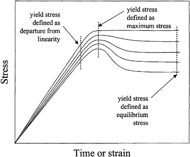Fig. 1 Schematical time evolution of the stress for imposed shear rate experiments at different imposed rates, and different attempts at defining a yield stress.⁶

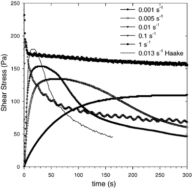Fig. 2 Time evolution of the stress for actual experiments for the same material at different imposed shear rates and different instruments.¹⁶

2.2 Shear localization

The H–B model and all analogous models suggest that all shear rates are possible in the material. However in practice, as soon as one makes an attempt to create a homogeneous flow, this generally fails: only a small region of the material actually moves, and the rest remains “solid”. There can be two reasons for this: either there is shear banding (localization), or there is wall slip. The latter can usually be controlled by using rough surfaces, and although very interesting, will not be considered here. Hence we focus on the shear localization. In rheological experiments the sample is usually assumed to be homogeneous and the local shear rate is derived from assuming that the globally imposed shear rate distributes accordingly throughout the sample. If shear banding occurs, this will of course not be the case, and much care must be exercised to avoid misinterpreting rheological data by implicitly assuming the shear rate to be distributed uniformly when a global shear rate is imposed macroscopically.

Using H–B like models, the only possible interpretation of shear localization is that there is a stress variation throughout the sample. Within the sheared region, the stress should then be higher than the yield stress, and outside that region it should be below. In a Couette geometry the stress usually varies as much as 10–20% and the H–B model allows in principle for a transition between a fluid and a solid region. However, in practice the H–B model predicts a much less abrupt transition than what is seen experimentally.^8,17 In addition shear localization is also observed for instance in cone-plate cells for which the stress is almost completely constant.^8–10† Interestingly such shear banding happens only under imposed shear rate and does not appear to be observable under an imposed stress, which also conflicts with H–B behavior. In addition to this, recent very precise experiments strongly suggest that shear localization is the rule below a critical shear rate,.¹⁷ Below this shear rate, all the flow is localized in a region close to the shearing wall. If the globally imposed shear rate is increased it is not the shear rate in the sheared region that increases, but rather the extent of the sheared region which grows—to fill the entire gap of the shear cell exactly at the critical shear rate.^8,17,19 See Fig. 3. Huang et al.¹⁷ show on a granular paste that the critical shear rate where the sheared region invades the entire gap (determined by MRI measurements) corresponds exactly to the shear rate for which an abrupt change occurs in the flow curve diagram as seen in Fig. 4. Wall slip is absent in all of these experiments (it would have been observed directly in the MRI experiments). All this therefore suggests that the shear localization is an intrinsic property of yield stress fluids, that always manifests itself at low enough shear rates. The manifestation is in this respect independent of the precise experimental protocol or measurement geometry.

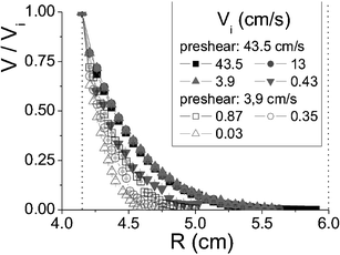Fig. 3 MRI measurements of the normalized velocity profile of a wet granular paste in a Couette geometry. It is seen that the shear localizes if the macroscopically imposed shear rate is below a certain limit. This limit is found to be 0.4 ± 0.1 s⁻¹.¹⁷

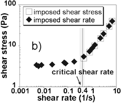Fig. 4 Imposed shear rate measurements on the same wet granular paste as in Fig. 3. The critical shear rate for transition between the two regions of the flow curve corresponds well with the critical shear rate for localization of shear found from Fig. 3.¹⁷

3 Thixotropic fluids, avalanche behavior and discontinuous viscosity—the way out

Thixotropic fluids are fluids with a variable viscosity which reversibly decreases with time under high shear rates. Because of the reversibility, in general the viscosity increases in time at low or zero shear rates.^7,11,20 For an experimental example of thixotropic behavior, see Fig. 5. The usual explanation of thixotropy is that the viscosity of such fluids is mainly caused by the microstructure of for instance particles in the fluid that interconnect and resist large rearrangements; for a recent detailed study, see Dullaert.²¹ When sheared, this structure is broken down in time and the viscosity consequently decreases in time. When left at rest, the microstructure slowly rebuilds itself and the viscosity increases.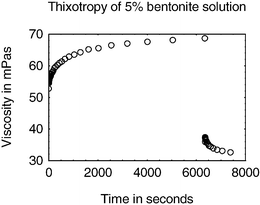

Fig. 5 Time evolution of the viscosity of a 5% bentonite solution under different imposed shear rates. The sample is pre-sheared at for 5000 s. Then a shear rate of 25 s⁻¹ is imposed for about 6000 s, after which the shear rate is changed back to 100 s⁻¹.

In the physics literature on soft glassy materials, these concepts have emerged recently; a viscosity increase of a sample left at rest is termed ‘aging’, in analogy to the aging of glasses, and the viscosity decrease in time under shear (thixotropy) is termed ‘shear rejuvenation’. Since there is no large-scale structure in glasses, the microscopic interpretation of these effects is different. However the competition between the two effects will also determine the mechanical behavior of these systems,^{7,11–14,22–25} and rheology experiments on soft colloidal glasses²² show a striking similarity to those on ‘typical’ yield stress fluids. For structured materials such as gels, the ‘aging’ and ‘rejuvenation’ are of course two aspects of the same phenomenon: the build-up and destruction of the microstructure. To retain the generality of our discussion here and include also glassy materials, we will therefore use aging and rejuvenation in the following, rather than build-up and destruction.

How are yield stress and thixotropy interrelated? A very striking demonstration of the interplay between the two is the ‘avalanche behavior’ recently observed for yield stress materials.¹⁴ One of the most simple tests to determine the yield stress of a given fluid is the so-called inclined plane test^26,27 A large amount of the material is deposited on a plane which is subsequently slowly tilted to some angle. According to the H–B model, the material will just start flowing when an angle is reached for which the yield stress equals the gravitational force per unit area σ_y = ρghsinθ, with ρ the density of the material, g the gravitational acceleration and h the height of the deposited material. In reality however, inclined plane tests on a clay suspension (bentonite)¹⁴ reveal that for a given thickness there is a critical slope above which the sample starts flowing. Once it is flowing, the thixotropy leads to a decrease in viscosity. Since fixing the angle implies fixing the stress, this will accelerate the flow. This in turn leads to an even more pronounced viscosity decrease and so on: an avalanche results, transporting the fluid over large distances, where an H–B fluid would move only infinitesimally when the critical angle is slightly exceeded (Fig. 6). In Fig. 7 the experimental data of such inclined plane experiments¹⁴ are compared with the H–B prediction which is clearly an inadequate description. It is interesting to compare the results of the inclined plane tests with experiments showing avalanches in granular materials - a situation for which there is a general agreement that avalanches exist. The exact same experiment had in fact been done earlier for a heap of dry sand, with results that are strikingly similar to those observed for the bentonite, see Fig. 8.

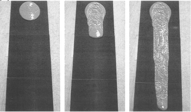Fig. 6 Avalanche flow of a clay suspension over an inclined plane covered with sandpaper. The experiment was performed just above the critical angle, below which the fluid behaves like a solid.¹⁴

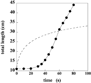Fig. 7 Distance covered by the fluid front in an inclined plane experiment.¹⁴ The experimental points are compared with the prediction of the H–B model (dashed line).

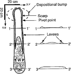Fig. 8 The inclined plane experiment with a heap of dry sand. The similarity of the resulting avalanche deposit with that of the clay avalanche is striking, especially the very characteristic ‘horseshoe’ form at the top of the plane.²⁹

In the more quantitative experiment accompanying the inclined plane test,¹³ a sample of 4.5% bentonite solution, which is a thixotropic fluid as can be seen in Fig. 5 was loaded in different geometries (Couette and plate–plate)‡—and for each experiment brought to the same initial state by a controlled history of shear and rest. Starting from this identical initial condition, different levels of shear stress were imposed on the samples and the viscosity was measured as a function of time. The result is shown in Fig. 9 and deserves some discussion. For stresses smaller than a critical stress, σ_c, the viscosity of the sample increases in time until the flow is halted altogether: the steady-state viscosity is infinite. On the other hand, for a stress only slightly above σ_c, the viscosity decreases with time towards a (low) steady state value η₀. The important point here is that the transition between these two states is discontinuous as a function of the stress. All this can be understood in terms of the competition between aging and shear rejuvenation.

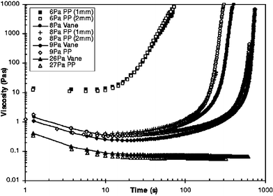Fig. 9 The time evolution of the viscosity of identical initial states with different applied stresses. A bifurcation in the steady state viscosity is seen to occur at a critical stress, σ_c between 9 and 26 Pa s.¹³

Aging

At rest or under very slow flow the fluid ages, and consequently its viscosity increases in time. This corresponds physically to the buildup of the colloidal gel of bentonite, and is indeed what is observed in the experiments: the viscosity increases in time without bound, and the end of the experiment corresponds to a viscosity that is too large to be measured accurately by the rheometer. This can be seen pragmatically as the absence of flow: for all stresses smaller than the critical stress the steady-state viscosity is infinite! Note that this is an ‘inverse avalanche’ effect, since the viscosity increases, the shear rate decreases, and the ‘aging’ becomes easier: this is the reason for which the measured viscosity increases faster near the end of the experiment.

Shear rejuvenation

However, the dominance of the aging process is only assured if the flow rate is small enough. In the experiment, for a stress that can be as little as 1% larger than that for which the aging predominates, the sample starts to flow. Subsequently, the flow destructures the material (breaks down the colloidal gel), which decreases the viscosity. This viscosity decrease causes an acceleration of the flow and so on: due to the avalanche effect discussed above, the steady state viscosity is low.

Consequently, there exists a critical stress that bounds a region of no flow for smaller stresses, and a region of fast flow for higher stresses. The conclusion is that there exists a whole range of steady state shear rates that are not accessible experimentally under an imposed stress: all shear rates between ‘fast’ flow and no flow at all. This also defines the critical shear rate as the lowest shear rate for which the sample still flows, i.e., the shear rate corresponding to the critical stress, σ_c. The steady-state viscosity jumps discontinuously from infinity to a finite and low value at σ_c, in sharp contrast with the continuous divergence of an H–B fluid, but agreeing with the conclusions from the inclined plane test. In addition, due to the aging effects the critical stress is no longer a property of the fluid: the longer one waits, the more the sample will age, and consequently the higher the critical stress will be. This again makes perfect sense for instance for the bentonite colloidal gel whose structure is continuously evolving; it explains some of the difficulties one experiences when measuring the yield stress; and it underlines the importance of the experimental protocol: only by controlling the aging history of the sample by a large pre-shear (and optionally a controlled period of rest subsequently), can reproducible results be obtained. An additional difficulty that is worthwhile mentioning in this respect is that the relation between the viscosity and the microstructure is a highly non-trivial one. Two samples of the same thixotropic fluid may have the same viscosity at a given shear rate, but a different structure. This is called ‘structural hysteresis’,^21,28 and underlines once more the importance of the (shear) history of the sample for its flow properties.

There seem to be very few if any examples of yield stress fluids which are not also thixotropic. Indeed the authors have not been able to find even one such example. The following ‘typical’ yield stress fluids have been investigated: foams, emulsions, colloidal gels, polymer gels (including carbopol), dry and wet granular materials. In addition, colloidal glasses show a behavior that is very similar, stressing the analogy between yield stress fluids and glassy materials proposed earlier.^30,31 Indeed, the yield stress and the thixotropy of a fluid originate from the same basic physics. For the bentonite example above, the colloidal gel that forms is both responsible for the yield stress - the percolated structure of clay particles confers the elasticity to the material - and the thixotropy: if the flow is strong enough it will partially destroy this structure and hence the viscosity will decrease. Since yield stress and thixotropy thus seem strongly connected and are properties of many (perhaps microscopically different) yield stress fluids, one might expect the same basic principle giving rise to both phenomena in all these different systems. Such a basic principle must be simple enough to be independent of specific system details in order to be generic for all thixotropic yield stress fluids. Since the competition between aging and shear rejuvenation is known to dominate the structure of the fluid which, in turn, causes both the yield stress and thixotropy, this interplay is a natural starting point for an attempt at a general description of these phenomena. In the following sections one such attempt will be examined and compared with experiments.

4 A simple yield stress model including thixotropy

A large number of models for thixotropy exist (see Dullaert²¹ for a recent overview) and depending on the degree of sophistication one wants to achieve, the models may become rather involved. We will consider here the simplest possible model, in order to establish the minimal ingredients of a model that qualitatively accounts for the behaviors reported above. The model therefore does not account for more complicated effects such as for example the ‘structural hysteresis’,²⁸ but will be very useful in understanding the basic physics of the problem.

A simple model taking into account the interplay between flow, structure and viscosity qualitatively captures the behavior of thixotropic yield stress fluids. The basic assumptions of the model are: (1) there exists a structural parameter, λ, that describes the local degree of interconnection of the microstructure. For the pertinent example of the bentonite colloidal gel, one may think of λ as a measure of the number of connections per unit volume. This can be measured directly, since the elastic modulus of a physical gel is generally taken to be proportional to the number of network connections per unit volume. For a glass, λ should be a measure of the depth of the local minimum in the energy landscape. For a granular material, one might think of it as a measure of how jammed the particles are on average. In a foam (suspension), it could be a combination of the same jamming and the rigidity of the individual bubbles (drops). (2) The viscosity increases with increasing λ. It turns out that if the dependence is sufficiently strong, a yield stress appears naturally. (3) For an aging system at low or zero shear rate, λ increases while if the flow breaks down the structure, λ decreases and reaches a steady state value at sufficiently high shear rates.

The simplest model that has these features consists of an evolution equation for λ:^13,14

coupled to an equation for the viscosity given by either of:η = η₀ exp(βλ) (model I), η = η₀ (1 + βλⁿ) (model II)

Here τ is the characteristic time of the build-up of the microstructure at rest and η₀ the limiting viscosity at high shear rates; α, β and n are parameters that should be specific for a given material. This simple description of a thixotropic yield stress fluid has a steady state solution

This relation can be used to find the steady state stress if a functional form of η(λ) is assumed. It is most instructive to look in detail at model II; for the steady-state viscosity, it follows that

which for high shear rates, when all the structure in the fluid is destroyed gives a Newtonian fluid behavior:
whereas for low shear rates the limiting behavior is

This last result shows that for a weak dependence of the viscosity on λ, 0 < n < 1 we find a simple shear-thinning fluid without a yield stress. However, for n > 1, a yield stress appears naturally within the model. As can be seen in Fig. 10, there exists a critical stress below which no steady state shear rate can be achieved. This will obviously give rise to yield stress behavior. The flow curve that follows from the model shows that for low shear rates the stress decreases with increasing shear rate, whereas for high shear rates it increases. This defines both a critical stress and a critical shear rate; these are both given by the minimum in the flow curve. For shear rates smaller than the critical shear rate the flow curve has a negative slope. This corresponds to a negative (absolute) viscosity, and signals unstable flows.

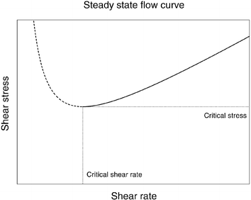Fig. 10 The steady state flow curve of model II with n = 2. The part to the left of the critical shear rate is dashed since the flow is unstable here and the homogeneous flow curve is very difficult to obtain.

The requirement for having an unstable flow is:

For model I this criterion translates into:

And for model II:

It is seen that for sufficiently small shear rates these criteria will be satisfied for any value of β (for model II again provided that n > 1).

Below, we will show that this rather simple addition of thixotropy to the yield stress behavior allows us to account qualitatively for all of the phenomena described above, and consequently solves most of the problems surrounding yield stresses.

5 Comparison with experiments

5.1 The yield stress and the problems with it

In this model, three parameters characterize the material in an experiment at any given time: the stress σ, the shear rate , and the structural parameter λ (and through it the viscosity η). If any two of these are given, the third can be found using the dependence . Now, consider a starting point (i.e. a pair ofand σ coordinates) for an experiment located at some point above the flow curve of Fig. 10. From eqn 1 it is seen that such a point will move towards lower values of λ—either down or to the right in the flow curve diagram depending on whether the shear rate or stress is imposed. Conversely, a starting point below the steady state curve will move towards higher values of λ either up (imposed shear rate) or to the left (imposed stress). Thus, given an initial value of λ one can predict the critical stress at which the aging exactly balances the rejuvenation. This is the stress corresponding to the intersection between the steady state flow curve and the straight line of the constant viscosity flow curve given by the initial value of λ. See Fig. 11. Above this stress the flow will speed up, below it will slow down. If the intersection is in the unstable region to the left of the critical shear rate, the long term change in shear rate will be very dramatic, so that the association of an ‘actual’ yield stress with this critical stress seems reasonable. However, it should be kept in mind that due to the aging, this yield stress is now a function of the time the sample has been given to rest, and is therefore not a material property, but rather dependent on both the material and on λ.

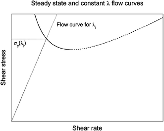Fig. 11 The intersection between the steady state flow curve and the straight line of the flow curve given by the initial value of λ, gives the value of the shear history dependent yield stress.

As already mentioned one popular way of finding the yield stress is to enforce a constant shear rate on a system and infer the yield stress from the stress over time curve. Based on the discussion above it can be understood why the obtained value depends on both the imposed shear rate and how the sample is treated prior to the experiment. It is also worthwhile noting that if λ is small initially, an applied stress that is below the critical stress could result in flows which might remain measurable for some time. Thus the yield stress is not the stress below which no flow occurs; the times necessary to reach the steady state corresponding to no measurable flows can be as long as an hour in our experiment. Thus a yield stress should be defined as the stress below which no permanent flows occurs. The following procedure allows for finding this newly defined material and history dependent yield stress. Several samples are prepared in an identical fashion (identical histories of pre-shear and rest) and each sample should be subject to a different but constant shear stress. After observing the long time behavior, the yield stress can be identified as the transition stress between the highest stress for which sample comes to a complete halt, and the lowest stress for which permanent flows are observed. This is actually the procedure followed in Fig. 9. The considerations above also demonstrate that the yield stress defined in this way is really not a material property, but depends on the value of λi.e. the shear history of the system. This we believe is at the heart of the ‘thixotropic obstacles in determining the yield stress’.¹⁶

5.2 The critical stress and avalanche behavior

Solved dynamically, the model reproduces both the bifurcation and the avalanche behavior. When the stress is imposed, in time the viscosity either tends towards infinity or to a small value depending on whether the stress is larger or smaller than the critical value σ_c, as is shown in Fig. 12. In the viscosity bifurcation experiments¹³ the sample is prepared in a certain reproducible initial state (i.e. value of λ) and different stresses are applied. If the shear rate history of the sample is such that the stress is smaller than the critical stress, the system will forever move to the left in the flow diagram towards an infinite viscosity. To the contrary, a stress just above the critical stress will make the system move to the right in the flow diagram until the intersection with the flow curve corresponding to a low viscosity and high shear rate. Thus, the viscosity jumps discontinuously to infinity at the critical stress, as was indeed observed in the experiments.^13,14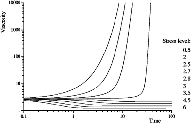

Fig. 12 Dynamical solution of the model equations. The graph shows how the viscosity evolves in time for different imposed shear stresses.¹³ The qualitative resemblance with the experimental data in Fig. 9 is striking.

5.3 The critical shear rate and shear banding

If on the other hand, the shear rate is fixed below the critical shear rate corresponding to the minimum of the flow curve, , the system can accommodate the globally imposed average shear rate by spatially dividing the system into two ‘phases’—one solid part, where the shear rate is zero, and one fluid part, which is sheared roughly at . The proportion of the fluid phase grows from zero to one when the average shear rate grows from zero to the critical value. Therefore, the shear localization observed in many experiments on yield stress fluids naturally comes out of the proposed model, and all the predictions of the model are in qualitative agreement with imposed shear rate experiments. The latter show that when the shear is sufficiently low localization occurs, and disappears exactly at the critical stress, in line with the conclusions from the model.^8,15,17

6 Comparison with models in the literature

Since the thixotropy of a large number of fluids has for a long time been very well established,^{7,11,13,14,32,33} many models for thixotropic behavior through a structural parameter have been proposed.^{12–14,24,25,34–37} Several of them are summarized by Barnes⁷ and in tabular form by Mujumdar et al.¹²

A class of models similar to our evolution equation for λ (we will call these λ-models in the following) have been used for a range of very different systems. For instance λ has been used to describe the degree of flocculation for clays,³⁸ as a measure of the free energy landscape for glasses,³⁹ or to give the fraction of particles in effective potential wells for colloidal suspensions.²⁶ This way of introducing an interconnection between the shear history and the viscosity of thixotropic systems was first proposed by F. Moore in 1959⁴⁰ (or in a slightly different wording, identical to the one used here, by Cross in 1965).³⁴ Generally the λ-models all assume:

where f is the rate of reconstruction (or aging) of the fluid and g is the rate of destruction (or shear rejuvenation). The complexity chosen for the right hand sides of eqns 2 and 3 may vary quite a bit from model to model.^{7,12–14,35–37,41}

The general assumption is that causes the slope of the flow curve diagram to be positive everywhere. This holds true for the flow curves of all the models summarized by Mujumdar et al.¹² and Barnes.⁷ This implies that the flows are stable: the negative slope is what leads to instability since a lower stress can sustain a higher shear rate. In a general mathematical treatment of the behavior of any λ-model by Cheng et al. in 1965,²⁵ the authors try to argue that the flow curve of all such models must have a positive slope everywhere. A very few of the papers summarized by Mujumdar et al.¹² and Barnes⁷ may have regions of negative slope of the flow curve for some parameter choices,^34,42 but the parameters required for this are avoided and the possibility of having unstable flows is not discussed. These models differ therefore significantly from the one explained above, that rationalizes the occurrence of shear localization and in which the yield stress appears naturally.

Very recently, Cheng investigated a model in which he did not presuppose the flow curve to have a positive slope everywhere.²⁴ His mathematical treatment however, does not consider the implications of the spatial extent of the fluid. This removes the possibility of shear banding and Cheng concludes that the region of the flow curve with negative slope, while unstable when constant stress is imposed, will not show any strange behavior if constant shear rate is imposed, which appears to disagree with experiment.

Most of the models summarized in the also recent paper by Mujumdar¹² introduce a yield stress manually, i.e. the σ_y term in eqn 3 is nonzero. Probably this is done because a yield stress is known to be present in many fluids, and the positive-only flow curves of the models cannot show yield stress behavior inherently. This ‘artificial’ yield stress seems unnecessary in view of the naturally occurring yield stress from the sections above.

7 Conclusion

Fluids that appear solid for stresses below a critical limit are called yield stress fluids, and are often modeled by yield stress fluid models such as the Herschel–Bulkley model. This review points out some fundamental conflicts between experiments on the one hand and the predictions of such models on the other hand. Indeed problems arise even with the definition and concept of a yield stress as the stress where the fluid just starts/stops flowing. Thixotropy is another prominent feature of many complex fluids and it indeed appears to be present whenever a yield stress is present also. Both phenomena are believed to be caused by the same underlying physics, but have traditionally been modeled as separate phenomena. This short review summarizes a number of recent experimental findings and presents the results of some recent developments within a group of models designed to describe the interplay between yield stress and thixotropy. These new developments allow for a very simple model to explain both thixotropy and yield stress behavior as two effects of the same cause: the interplay between flow and structure of a fluid. This simple model provides a qualitative explanation of many if not all features of real yield stress fluids that are incompatible with the ideal picture of a yield stress. Notably, it suggests that shear localization is an intrinsic property of yield stress fluids, that always manifests itself at low enough shear rates. The experimental data and the understanding brought forth by the new model beg for a redefinition of the concept of the yield stress, which is suggested here.

References

1. E. C. Bingham, Fluidity and Plasticity. McGraw-Hill, New York, 1922.
2. R. B. Bird, G. C. Dai and B. Y. Yarusso, The rheology and flow of viscoplastic materials, Rev. Chem. Eng., 1982, 1, 1–70.
3. Q. D. Nguyen and D. V. Boger, Measuring the flow properties of yield stress fluids, Annu. Rev. Fluid. Mech., 1992, 24, 47–88.
4. H. A. Barnes, The yield stress—a review or ‘παντα ρει’—everything flows?, J. Non-Newtonian Fluid Mech., 1999, 81, 133–178.
5. A. E. James, D. J. A. Williams and P. R. Williams, Direct measurement of static yield properties of cohesive suspensions, Rheol. Acta, 1987, 26, 437–446.
6. H. A. Barnes and Q. D. Nguyen, Rotating vane rheometry - a review, J. Non-Newtonian Fluid Mech., 2001, 98, 1–14.
7. H. A. Barnes, Thixotropy - a review, J. Non-Newtonian Fluid Mech., 1997, 70, 1–33.
8. P. Coussot, J. S. Raynaud, F. Bertrand, P. Moucheront, J. P. Guilbaud, H. T. Huynh, S. Jarny and D. Lesueur, Coexistence of liquid and solid phases in flowing soft-glassy materials, Phys. Rev. Lett., 2002, 88, 218301.
9. F. Pignon, A. Magnin and J.-M. Piau, Thixotropic colloidal suspensions and flow curves with minimum: Identification of flow regimes and rheometric consequences, J. Rheol., 1996, 40, 573–587.
10. M. M. Britton and P. T. Callaghan, Nuclear magnetic resonance visualization of anomalous flow in cone-and-plate rheometry, J. Rheol., 1997, 41, 1365–1386.
11. J. Mewis, Thixotropy - a general review, J. Non-Newtonian Fluid Mech., 1979, 6, 1–20.
12. A. Mujumdar, A. N. Beris and A. B. Metzner, Transient phenomena in thixotropic systems, J. Non-Newtonian Fluid Mech., 2002, 102, 157–178.
13. P. Coussot, Q. D. Nguyen, H. T. Huynh and D. Bonn, Viscosity bifurcation in thixotropic, yielding fluids, J. Rheol., 2002, 46, 573–589.
14. P. Coussot, Q. D. Nguyen, H. T. Huynh and D. Bonn, Avalanche behavior in yield stress fluids, Phys. Rev. Lett., 2002, 88, 175501.
15. J. C. Baudez and P. Coussot, Abrupt transition from viscoelastic solidlike to liquidlike behavior in jammed materials, Phys. Rev. Lett., 2004, 93, 128302.
16. J. R. Stokes and J. H. Telford, Measuring the yield behavior of structures fluids, J. Non-Newtonian Fluid Mech., 2004, 124, 137–146.
17. N. Huang, G. Ovarlez, F. Bertrand, S. Rodts, P. Coussot and D. Bonn, Flow of wet granular materials, Phys. Rev. Lett., 2005, 94, 028301.
18. D. C.-H. Cheng, Cone-and-plate viscometry: explicit formulae for shear stress and shear rate and the determination of inelastic thixotropic properties, Br. J. Appl. Phys., 1966, 17, 253–263.
19. V. Bertola, F. Bertrand, H. Tabuteau, D. Bonn and P. Coussot, Wall slip and yielding in pasty materials, J. Rheol., 2003, 47, 1211–1226.
20. R. G. Larson, The Structure and Rheology of Complex Fluids, Oxford University Press, Oxford and New York, 1999.
21. K. Dullaert, Constitutive equations for thixotropic dispersions. PhD thesis, Katholieke Universiteit Leuven, 2005.
22. B. Abou, D. Bonn and J. Meunier, Aging dynamics in a colloidal glass, Phys. Rev. E: Stat. Phys., Plasmas, Fluids, Relat. Interdiscip. Top., 2001, 64, 021510.
23. L. Berthier, J.-L. Barrat and J. Kurchan, A twotime-scale, two-temperature scenario for nonlinear rheology, Phys. Rev. E: Stat. Phys., Plasmas, Fluids, Relat. Interdiscip. Top., 2000, 61, 5464–5472.
24. D. C.-H. Cheng, Characterisation of thixotropy revisited, Rheol. Acta, 2003, 42, 372–382.
25. D. C.-H. Cheng and F. Evans, Phenomenological characterization of the rheological behaviour of inelastic reversible thixotropic and antithixotropic fluids, Br. J. Appl. Phys., 1965, 16, 1599–1617.
26. P. Coussot and C. Ancey, Rheophysics of Pastes and Suspensions. EDP Sciences, Paris, 1999.
27. P. Coussot and S. Boyer, Determination of yield stress fluid behaviour from inclined plane test, Rheol. Acta, 1995, 34, 534–543.
28. J. Mewis, A. J. B. Spaull and J. Helsen, Structural hysteresis, Nature, 1975, 253, 618–619.
29. R. R. McDonald and R. S. Anderson, Constraints on eolian flow dynamics through laboratory experiments on sand slopes, J. Sedimentary Res., 1996, 66, 642.
30. D. Bonn, P. Coussot, H. T. Huynh, F. Bertrand and G. Debrégeas, Rheology of soft glassy materials, Europhys. Lett., 2002, 59, 786–792.
31. F. Varnik, L. Bocquet, J.-L. Barrat and L. Berthier, Shear localization in a model glass, Phys. Rev. Lett., 2003, 90, 095702.
32. F. Pignon, A. Magnin and J.-M. Piau, Thixotropic behavior of clay dispersions: combinations of scattering and rheometric techniques, J. Rheol., 1998, 42, 1349–1373.
33. B. Abou, D. Bonn and J. Meunier, Nonlinear rheology under an external drive, J. Rheol., 47, 2003, 47, 979–988.
34. M. M. Cross, Rheology of non-newtonian fluids: A new flow equation for pseudoplastic systems, J. Colloid Sci., 1965, 20, 417–437.
35. C. F. Chan Man Fong and D. De Kee, Yield stress and small amplitude oscilatory flow in transient networks, Ind. Eng. Chem. Res., 1994, 33, 2374–2376.
36. D. Soong and M. Shen, Kinetic network model for nonlinear viscoelastic properties of entangled monodisperse polymers i. steady-state flow, J. Rheol., 1981, 25, 259–273.
37. D. De Kee, R. K. Code and G. Turcotte, Flow properties of time-dependent foodstuffs, J. Rheol., 1983, 27, 581–604.
38. D. Quemada, Rheological modelling of complex fluids: iv thixotropic and thixoelastic behavior. startup and stress relaxation, creep tests and hysteresis cycles, Eur. Phys. J.: Appl. Phys., 1999, 5, 191–207.
39. J. P. Bouchaud, A. Comtet and C. Monthus, On a dynamical model of glasses, J. Phys. I, 1995, 5, 1521–1526.
40. F. Moore, The rheology of ceramic slip and bodies, Trans. Br. Ceramic Soc., 58, 470–494.
41. S.-F. Lin and R. S. Brodkey, Rheological properties of slurry fuels, J. Rheol., 1985, 29, 147–175.
42. A. W. Sisko, The flow of lubricating greases, Ind. Eng. Chem., 1958, 50, 1789–1792.

---

Footnotes

† The stress in a cone-plate geometry is not entirely constant, but has a typical variation of less than 1%, which in a H–B setting should give shear banding only if the imposed average stress is within 1% of the yield stress. Hence this cannot explain the numerous situations in which shear banding is observed. For a detailed study of stresses in a cone-plate geometry see Cheng¹⁸

‡ Interestingly, in contrast with many experimental tests the results seem independent of the geometry.

---