DOI:
10.1039/B212786E
(Paper)
PhysChemComm, 2003,
6, 28-31
Origin of the sub-diffusive behavior and crossover from sub-diffusive to super-diffusive dynamics near a biological surface
Received
7th January 2003
, Accepted 20th March 2003
First published on 31431st March 2003
Abstract
Diffusion of a tagged particle near a constraining biological surface is examined numerically by modeling the surface-water interaction by an effective potential. The effective potential is assumed to be given by an asymmetric double well constrained by a repulsive surface towards r
→ 0 and unbound at large distances. The time and space dependent probability distribution P(r,t) of the underlying Smoluchowski equation is solved by using the Crank–Nicholson method. The mean square displacement shows a transition from sub-diffusive (exponent α
≈ 0.46) to a super-diffusive (exponent α
≈ 1.75) behavior with time and ultimately to diffusive dynamics. The decay of self intermediate scattering function (Fs(k,t)) is non-exponential in general and shows a power law behavior at the intermediate time. Such features have been observed in several recent computer simulation studies on the dynamics of water in proteins and micellar hydration shells. The present analysis provides a simple microscopic explanation for the transition from the sub-diffusivity and super-diffusivity. The super-diffusive behavior is due to escape from the well near the surface and the sub-diffusive behavior is due to the return of quasi-free molecules to form the bound state again, after the initial escape.
1 Introduction
The dynamics of the water molecules in the vicinity of a biological surface are found to be different from those in the bulk.1–10 The dynamical properties of water around a protein surface are found to depend on the distance from the biomolecular surface.1–3,9 Similar observations have been obtained from the computer simulations of water near micellar surface.10 In particular, the mean square displacement (MSD) of water molecules close to biological surfaces is found to be sublinear with time.2,3,11 These results have been confirmed by neutron scattering experiments also.12 MSD can in general be written as below,| | | MSD =
〈|Δr(t)|2〉
=
c
+
a
×
tα | (1) |
where |Δr(t)| is the displacement of a molecule at time t. For diffusive dynamics, α
= 1. For sub-diffusive dynamics α < 1, whereas the dynamics is called super-diffusive if α > 1. Recent computer simulation studies by Cannistraro et al. showed that the dynamics of water near a constrained biological surface is sub-diffusive for short time (below 10 ps) with the exponent α varying from 0.75 to 0.96 depending on the region of water molecules chosen at different distances from the protein surface.13,2 Sub-diffusivity has been observed in many other types of systems also, such as membrane bound protein,14 polymer melts,12,15–17 and the transverse motion of membrane point due to the bending modes18etc. On the other hand, enhanced or super-diffusion with an exponent 1.5 has been observed in the mean square displacement of engulfed microsphere in a living eukaryotic cell,19,20 with a sub-diffusive behavior at short times.21 The occurrence of super-diffusion has been interpreted as the evidence for a generalized Einstein relation, whereby the motion of the particles along microtubules in a dense network require displacement of the surrounding filaments. The time dependent diffusion coefficient is related by time dependent viscosity of the medium.21 Recently, Garcia and Hummer reported a study on the dynamics of cytochrome c which exhibits a crossover from sub-diffusive over a short period (below 100 ps) to super-diffusive dynamics in the longer time with exponents 0.5 and 1.75, respectively.22 Origin of the crossover from sub-diffusive dynamics at short time (t
≤ 10 ps) to super-diffusive dynamics at intermediate time (10 ps ≤
t
≤ 200 ps) for different systems is not yet fully understood.
Observations for the sub-diffusive dynamics of water near the biological surface have often been attributed to enhanced stability of the water molecules at the surface due to hydrogen bonding to the biological surface.23–26 Theoretical models have been developed in terms of bound ⇌ free equilibration.27 The evidence of such exchange was obtained by a nuclear Overhauser effect experiment.28 On the other hand, molecular dynamics simulations of water molecules at protein and micellar surfaces show the existence of sizable fraction of water molecules in the layer with residence time larger than the rest.29 The binding energy distribution varies from 0.5 to 9 kcal mol−1. The trajectory of individual water molecules clearly shows a dynamic equilibrium, between a bound state and a free state.30,31 To the best of of our knowledge, no simple explanation has been offered for the observed super-diffusive behavior.
Note that no detailed numerical solutions of time dependent diffusion or time dependent mean square displacement (MSD) in the model bistable potential have been carried out, even though such a study can throw light on the origin of the observed behavior. However, purely analytical studies in these type of systems have been limited by the fact that the heterogeneous surface faced by the water molecules makes a general analytical solution virtually impossible.
It is shown in recent simulations of a micelle that the bound water molecules are energetically stable with a potential energy contribution of 9–12 kcal mol−1 while the quasi-free water molecules which surround the bound water are only stable by 5–6 kcal mol−1.32 Radial distribution function (g(r)) shows that the first shell of water molecules shows a peak around 3.5 Å while the second shell shows a peak around 6–7 Å.32 The structure of g(r) suggests the existence of an effective binding potential which could be double well in nature because the effective potential is related to radial distribution function by the following well-known relation
In this work, we explain the origin of both the sub- and the super-diffusive behavior of the biological water by studying the diffusion over simple double well and Morse type of potentials. The double well potential represents the potential environment of the water close to a biomolecule. The first potential energy well corresponds to the bound water molecule and the second well corresponds to the quasi-free water molecule. The effective potential energy of interaction between the surface and the water molecules of course becomes negligible at a few layers from the surface and here the water is free and behaves as in bulk water. A model of free diffusion (without any potential) is studied to compare the dynamics of the biological water relative to the bulk water. We demonstrate by numerical computation of the probability density P(r,t) on the potential energy landscape that this model is able to catch the dynamical anomalies present in the biological water. The sub-diffusive behavior is shown to originate not only because of the binding to the surface but also due to the bound ⇌ free dynamic equilibration present among the water molecules at the surface. The MSD calculated from the distribution P(r,t) shows a cross-over from sub-diffusive behavior over a short time to a super-diffusive nature over a long time, precisely of the type observed in computer simulations.22 However, we find that a pronounced sub-diffusivity is present only when the exchange between the two wells is facile. Self intermediate scattering function Fs(k,t) calculated from P(r,t) also shows a marked non-exponential relaxation.
2 Model and numerical technique
Two Morse potentials are combined together to form different models of double well potentials. The two wells are constructed in such a way so that the separation between the wells are r0, 2r0, 3r0 in Model I, Model II and Model III, respectively. In the case of all the double well potentials, the depth of the first well is taken as −10 kBT and the second well is −7 kBT. A simple Morse potential with a well depth of −10 kBT is termed as Model IV. Simulations have also been done without the presence of any potential (free diffusion) which is termed as Model V. Fig. 1 shows the form variation of the potentials with distances from a constrained surface. All the model potentials reach zero at long distances. The double well potentials represent the stabilities of the first and second coordination shell of the water molecules surrounding the biological surface. The models have been constructed with different separations of double well to monitor the dynamics in the well and also the effect of exchange on the dynamics of water. For Model I and Model II, the two wells are close and that will facilitate the exchange, whereas in the case of Model III the exchange is hindered. The Morse potential (Model IV), on the other hand, has no second well to perform the exchange. The dynamics of the probability distribution P(r,t) is governed by a simple Smoluchowski equation as given below,| | 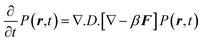 | (3) |
where, β
= 1/kBT and F is the force obtained from the derivative of underlying potential(E), F=
−∇E. Without the angular dependence, the radial part of the above equation takes a simple form as given below,| |  | (4) |
where g
=
∇.F. D is taken to be constant.
 |
| | Fig. 1 Potential energy diagram for different models used in this study. Models I, II and III are double well potentials. Model IV is a simple Morse potential and Model V is a free diffusion model without any potential. | |
The numerical solution of partial differential equation is a non-trivial task. The stability of the solution always depends on the equation type, variation of the potential and proper discretization of the equation. Here, the propagation of the distribution function is solved numerically by the Crank–Nicholson technique.33 This is an unconditionally stable method for the solution of parabolic type of equation. The numerical solution of a parabolic differential equation by the Crank–Nicholson procedure is described by a simple differential equation as below,
| |  | (5) |
where ℋ is the total Hamiltonian of the system. The formal solution of the above equation is,
The above equation can be discretized as below,
| |  | (7) |
where
n is the time index and
j is the space index. This is a half implicit scheme and the above equation can be solved by inverting a tridiagonal matrix. Although the procedure is unconditionally stable, proper care should be taken with the discretization of time and distance. The force has been calculated by using a cubic spline method where the two Morse potentials are joined to avoid the discontinuity. The distance
r is scaled by the
r0
= 3.5 Å where the first peak of radial distribution function appears for the
water around a biological surface. The time
t is scaled by
τ obtained from the diffusion of
water (
Dw) in the bulk water at 300 K,
τ
=
r20/(6
Dw)
= 8.5 ps, where
Dw
= 2.5 × 10
−5 cm
2 s
−1. The initial distribution of
P(
r,
t)
(at
t
= 0) is taken to be a very steep function (nearly delta function) peaked at
r
=
r0. Time step Δ
t is taken as 0.0001
τ and Δ
r is taken as 0.05
r0. Simple explicit differentiation scheme also works in this case.
3 Results and discussion
Fig. 2(a) shows the normalized probability distribution of r2P(r,t) at time t
= 200τ for all the model potentials. P(r,t) becomes non-Gaussian for the double and single well model potentials. Fig. 2(b) shows the normalized probability distribution for the free diffusion model. In case of double well potential r2P(r,t) forms bimodal distribution at intermediate time. Mean square displacement is calculated from r2P(r,t) using the equation below,| |  | (8) |
Mean square displacement shows different extent of sub-diffusive behavior over a short period depending on the nature of the model potentials. The cross-over to a super-diffusive behavior takes place in the intermediate time and finally the dynamics become diffusive. This dynamical dis-symmetry is depicted in the values of exponent α obtained from the fitting of MSD with eqn. (1) for the different models in different time windows. Table 1 shows the exponents α obtained for the model potentials in different time window.
 |
| | Fig. 2 (a) Probability distribution r2P(r,t) is plotted for short distances at time t = 200τ. All the models except the free diffusion show the non-Gaussian bimodal distribution. (b) The distribution r2P(r,t) is shown for Model V (free diffusion). | |
Table 1 The signature of the crossover from sub-diffusive to super-diffusive dynamicsa
| Model |
Sub-diffusive α |
Super-diffusive α |
| 0.3 → 10τ |
0.3 → 20τ |
20 → 200τ |
0.3 → 600τ |
|
Exponents from the fitting of MSD with eqn. (1) for different models in different time window.
|
| Model I |
0.03 |
0.96 |
1.76 |
1.65 |
| Model II |
0.58 |
0.46
|
1.75 |
1.64 |
| Model III |
0.96 |
0.97 |
1.76 |
1.81 |
| Model IV |
1.03 |
1.39 |
1.79 |
1.68 |
| Model V |
1.00 |
0.96 |
1.00 |
1.00 |
It is clear from the values of the exponents in Table 1 that over a short period (less than 10τ) most of the model potentials show sub-diffusive behavior. However, the sub-diffusivity persists for longer time (up to 20τ) in the case of Model II in which the exchange between the two wells is facilitated. All the models show super-diffusive dynamics in the intermediate time with exponents much higher than 1.0. In the very long term (above ≈200τ), diffusive dynamics starts setting in. So the exponent decreases in the fit for the larger time window. Model V shows simple diffusion in the absence of potential with exponent always equal to 1.0. Fig. 3 shows the MSD against for short time of 20τ. Fitting of Model II with eqn. (1) with a very low exponent is also shown in the same figure. Dynamics of MSD changes to a super-diffusive behavior in the longer time (beyond 10–20τ) as shown in Fig. 4. All the models show a pronounced super-diffusive dynamics although the overall MSD is much less compared to the diffusion of the free molecules as given by Model V. The exponent α obtained from the fit of the MSD are given in Table 1.
 |
| | Fig. 3 Sub-diffusive behavior of MSD over a short period for all the models. The sub-diffusive behavior is most prominent for Model II. Free particle diffusion for Model V is simple diffusive. | |
 |
| | Fig. 4 Super-diffusive time dependence of MSD for all the different models. All the models (except Model V) show super-diffusive behavior. However, the overall diffusion for all the models is much less compared to free particle diffusion. | |
Some nice correlations could be drawn from the change in the exponent of diffusion in the sub-diffusive and super-diffusive. The more pronounced sub-diffusive dynamics shows a less pronounced super-diffusive behavior. The slowing down in the dynamics due to the binding with the surface is reflected in the self intermediate scattering function Fs(k,t). Fig. 5 shows the non-exponential time dependence of the Fs(k,t) for all the different models at k
=
π/8. For the free diffusion, the dynamics of Fs(k,t) is exponential as expected. For all the other models, the non-exponentiality originates from the very slow relaxation of the system. The pronounced sub-diffusive behavior is reflected in the short time dynamics of Fs(k,t) in the case of the Model II. Similar signature of sub-diffusive dynamics is observed in the case of the second-rank dipole–dipole correlation function of lysozyme in water from computer simulation.34 Mode coupling theory of glassy liquids provide an explanation for the sub-diffusive behavior in terms of 〈Δr2(t)〉 and self intermediate scattering function. Fs(k,t) can be expressed from a Gaussian approximation as,
| |  | (9) |
where
A is a numerical constant related to diffusion. Clearly for
α not equal to unity,
Fs(
k,
t) becomes non-exponential.
F(
k,
t) plotted in
Fig. 5 have been fitted to stretched exponential and the exponents obtained are considerably less than unity in all the models except for the free diffusion which models the bulk water is purely exponential which is consistent with the relaxation properties observed in bulk
water.
24
 |
| | Fig. 5 Self intermediate scattering function (Fs(k,t)) is plotted against Log(t/τ) for all the models at k = 2π. Due to slow diffusion, all the models (except Model V) show non-exponential relaxation. Fs(k,t) for Model II over a short period shows the signature of sub-diffusive relaxation (see text). | |
4 Conclusion
Recent observations regarding the slow orientational and translational dynamics of the biological water compared to the bulk water is mapped to a simple problem of diffusion over a double well potential. The first well corresponds to the first coordination shell where the water is strongly hydrogen bonded to the biological surface and enthalpically very stable. The second well corresponds to the relatively free water which constitutes the second coordination shell. Diffusion over such a potential landscape is shown to mimic the recent experimental and simulation studies showing a cross-over from sub-diffusive to super-diffusive dynamics. Sub-diffusive dynamics originates not only from the relative stability of the potential well, but also from the backward diffusion process from the second well to the first well. The slow long time relaxation is reflected from the stretched exponential behavior of Fs(k,t). The present study provides convincing evidence that the binding to a constrained surface along with exchange between the free and bound water could be the primary reason for the sub-diffusive dynamics of biological water. In view of the results obtained in this work, the origin of super-diffusivity can be explained by a Heaviside step function representation of MSD as given by,| |  | (11) |
where P(ε) is the probability distribution of the potential energy of binding (ε), a is the separation between two wells (around 3 Å), DT is the translational diffusion coefficient, kbf and kfb are rate of conversion from bound to free and free to bound, respectively, and H(t) is the Heaviside step function, which is equal to unity for positive values of its argument and zero otherwise. So if the rate of conversion from bound to free is large, then the MSD will show a super-diffusive behavior. However, the free to bound transition retards diffusion and gives rise to sub-diffusive behavior. Note that free to bound transition is faster than bound to free because of much lower activation barrier in the former case.
Acknowledgements
We thank R. K. Murarka for technical discussions. Authors thank CSIR, New Delhi, India and DST, India for financial support.
References
- V. Lounnas, B. M. Pettitt and G. N. Phillips, Jr., Biophys. J., 1994, 66, 601 CAS.
- A. R. Bizzarri and S. Cannistraro, Phys. Rev. E, 1996, 53, 3040 CrossRef.
- A. R. Bizzarri and S. Cannistraro, Europhys. Lett., 1997, 37, 201 Search PubMed.
- S. Vajda, R. Jimnez, S. J. Rosenthal, V. Fidler, G. R. Fleming and E. W. Castner, J. Chem. Soc., Faraday Trans., 1995, 91, 867 RSC.
- S. Pal, J. Peon, B. Bagchi and A. H. Zewail, J. Phys. Chem. B, 2002, 106, 12376 CrossRef CAS.
- N. E. Levinger, Curr. Opin. Colloid Interface Sci., 2000, 5, 118 Search PubMed; R. E. Riter, D. M. Willard and N. E. Levinger, J. Phys. Chem. B, 1998, 102, 2705 CrossRef CAS.
- R. Jimnez, G. R. Fleming, P. V. Kumar and M. Maroncelli, Nature (London), 1994, 369, 471 CrossRef CAS.
- N. Nandi, K. Bhattacharyya and B. Bagchi, Chem Rev., 2000, 100, 2013 CrossRef CAS; K. Bhattacharyya and B. Bagchi, J. Phys. Chem. A, 2000, 104, 10603 CrossRef CAS.
- M. Levitt and R. Sharon, Proc. Natl. Acad. Sci. USA, 1988, 85, 7557 CAS.
- S. Balasubramanian and B. Bagchi, J. Phys. Chem. B, 2001, 105, 12529 CrossRef CAS; S. Balasubramanian and B. Bagchi, J. Phys. Chem. B, 2002, 106, 3668 CrossRef CAS.
- A. R. Bizzarri, C. Rocchi and S. Cannistraro, Chem. Phys. Lett., 1996, 263, 559 CrossRef CAS.
- G. D. Smith, W. Paul, M. Monkenbusch and D. Richter, Chem. Phys., 2000, 261, 61 CrossRef CAS.
- C. Rocchi, A. R. Bizzarri and S. Cannistraro, Phys. Rev. E, 1998, 57, 3315 CrossRef CAS.
-
C. Favard, N. Olivi-Tran and J.-L. Meunier, cond-mat/0210703, 2002, http://arxiv.org/abs/cond-mat/0210703.
- W. Paul, G. D. Smith, D. Y. Yoon, B. Farago, S. Rathgeber, A. Zirkel, L. Willnber and D. Richter, Phys. Rev. Lett., 1998, 57, 843.
- A. Kopf, B. Dünweg and W. Paul, J. Chem. Phys., 1997, 107, 6945 CrossRef CAS.
- W. Paul, K. Binder, D. W. Heermann and K. Kremer, J. Chem. Phys., 1991, 95, 7726 CrossRef CAS.
- R. Granek, J. Phys. II (Les Ulis, France), 1997, 7, 1761 Search PubMed.
- A. Caspi, R. Granek and M. Elbaum, Phys. Rev. Lett., 2000, 85, 5655 CrossRef CAS.
- A. G. Zilman and R. Granek, Chem. Phys., 2002, 284, 195 CrossRef CAS.
- H. Salman, Y. Gil, R. Granek and M. Elbaum, Chem. Phys., 2002, 284, 389 CrossRef CAS.
- A. E. Garcia and G. Hummer, Proteins, 1999, 36, 175 CrossRef CAS.
- M. J. Saxton, Biophys. J., 1996, 70, 1250 CAS.
- J.-P. Bouchaud and A. Georges, Phys. Rep., 1990, 195, 127 CrossRef.
- J. W. Haus and K. W. Kher, Phys. Rep., 1987, 150, 263 CrossRef CAS.
- S. Havlin and D. Ben-Abraham, Adv. Phys., 1987, 36, 695 CAS.
- N. Nandi and B. Bagchi, J. Phys. Chem., 1997, 101, 10954 Search PubMed.
- O. Gottfried, L. Edvards and K. Wuthrich, Science, 1991, 254, 974.
- S. Balasubramanian, S. Pal and B. Bagchi, Phys. Rev. Lett., 2002, 89, 115505 CrossRef.
- X. Cheng and B. P. Schoenborn, J. Mol. Biol., 1991, 220, 381 CAS.
- W. Gu and B. P. Schoenborn, Proteins: Struct., Funct., Genet., 1995, 22, 20 CAS.
-
S. Pal, S. Balasubramanian and B. Bagchi, J. Phys. Chem., submitted Search PubMed.
-
W. F. Ames, Numerical Methods for Partial Differential Equations, New York Academy Press, 2nd edn., 1977 Search PubMed; A. Goldberg and H. M. Schey, Am. J. Phys., 1967, 35, 177 Search PubMed.
- M. Marchi, F. Sterpone and M. Ceccarelli, J. Am. Chem. Soc., 2002, 124, 6787 CrossRef CAS.
|
| This journal is © The Royal Society of Chemistry 2003 |
Click here to see how this site uses Cookies. View our privacy policy here.