Ultrafast μLIBS imaging for the multiscale mineralogical characterization of pegmatite rocks

Abstract

This article presents an innovative application of kHz regime μLIBS – Laser-Induced Breakdown Spectroscopy for generating detailed compositional maps of geological samples. The method effectively covers large areas (tens of cm²) rapidly while maintaining high lateral resolution (below 20 μm), producing some of the most extensive LIBS compositional images to date, with a size of 10 million pixels. Employing elemental-based images, we developed a direct methodology for mineral phase identification through mask-creation operations and logical relationships. This approach was successfully applied to reconstruct the mineralogical map of a Li-ore from the west-European Variscan belt, identifying 14 different mineral phases, including economically valuable ones like lepidolite, cassiterite, and columbite-group minerals. Furthermore, based on the reverse normative calculation, the chemical composition of the sample was calculated from the mineral phases previously obtained. The kHz μLIBS approach marks a significant advancement in elemental and phase imaging, especially pertinent to geological applications, providing comprehensive petro-geochemical insights, essential for a fast geological characterization.

---

Introduction

Within its broad spectrum of potential applications, Laser-Induced Breakdown Spectroscopy (LIBS) analysis is particularly suitable for Earth Science.^1,2 Comprehensive mineralogical and petrographic studies require analytical methods to identify and quantify the spatial distribution of major and trace elements. In Earth Science laboratories, the most commonly used analytical techniques for geochemical characterization remain EMPA (Electron Micro Probe Analysis), LA-ICP-MS (Laser Ablation Inductively Coupled Plasma Mass Spectrometry), μXRF (micro X-Rays Fluorescence), and SIMS (Secondary Ion Mass Spectrometry). Some of these methods allow obtaining information on specific locations and elementary imaging for restricted millimetric zones for EMPA and SIMS. Larger surfaces can be analyzed with LA-ICP MS³ and μXRF,⁴ reaching the area of small rock sections (few cm²) or even larger in the case of μXRF.

LIBS is an analytical technique based on the spectroscopic analysis of the emission emitted by the species contained in a laser-induced plasma. When a laser interacts with a material, once the fluence per pulse exceeds a threshold value, it ablates a tiny amount of the sample (below ng per pulse), generating a plasma, the composition of which is indicative of the interaction zone. The emission of the excited species of this plasma, neutral, ionic, and molecular species, can be thus measured to obtain information about the sample composition.

Regarding its application in Earth Science, on one hand, the availability of portable instruments,^5–11 together with the capability of carrying out remote and stand-off analysis,^12–14 pushes LIBS analytical capabilities to the field, permitting it to be used for geochemical exploration and mapping at the scale of an outcrop or region and rock sampling optimization. On the other hand, the limited sample preparation requirements and the high spatial resolution (in the order of a few micrometers) make LIBS an invaluable tool for carrying out the chemical characterization of rocks and minerals in laboratories.

Due to the small size of the ablation zone, it is possible to reconstruct the 2D spatial representation of the sample composition. LIBS imaging has been applied to a wide range of fields, such as geological, industrial, forensic, or bio-medical applications.^15–20 Furthermore, all atoms are potential light emitters in the optical range from UV to IR and each possesses a specific signature, which we can detect via LIBS. A single laser shot can thus simultaneously detect light and heavy elements. The compositional imaging by LIBS, operating under ambient conditions and ultra-fast laser frequency up to kHz,^21–23 becomes very competitive with more conventional imaging techniques. LIBS can generate automated mineralogical recognition of rocks with a lateral resolution of 10 μm to 100 μm, with insights about their enrichment in economically important elements, even at low concentrations.^18,23–26

Nowadays, μLIBS imaging (i.e., with crater size and shot-to-shot distance in the order of a few micrometres) provides access to the distribution of trace, minor and major elements within different mineralogical phases of large samples of several cm². Contrary to μXRF or EMPA, LIBS is particularly appropriate for the analysis of light elements such as H, Li, Be, B, and C; halogens;^27,28 as well as first-row transition elements of the periodic table. They exhibit, in addition, a simpler optical response (a few emission lines), while sub-ppm sensitivity can be reached for some of these elements. As a recent illustration, Li-rich rock has been analyzed with μLIBS imaging, involving the examination of pegmatite drill cores sourced from the Rapasaari lithium deposit with a semi-supervised mineral classification of extensive samples.²⁹ The study utilized a frequency of 20 Hz and an ablation crater size of 200 μm. Mineralogical imaging was successfully achieved for four major minerals (quartz, spodumene, muscovite, and albite) across four distinct areas of few cm². The authors highlight the potential significance of matrix effects in Li-bearing pegmatites to explain the high variability observed in the physical properties of mineral grains.²⁹ In a parallel approach to drill core analysis, the authors employed a multivariate method, utilizing extensive training data through pixel-matched reference maps obtained via LA-ICP-TOFMS.³⁰ By combining LA-ICP-TOFMS and LIBS, the authors achieved rapid and precise spatial quantification of Li₂O and other major rock-forming elements in centimetric areas of a Li-bearing pegmatite drill core. However, the used spatial resolution of approximately 200 μm limits the identification of small mineral phases, a limitation overcome by μLIBS imaging as deployed in this study. The present study overcame this limitation using μLIBS imaging with 1 order of magnitude better resolution (<20 μm).

In this context, standard μLIBS imaging systems (typically with frequencies below 100 Hz) provide a tolerable experiment time for most applications on small-size samples. However, faster systems become preferable when large areas are studied at high spatial resolution. Increasing the laser shooting rate up to kHz levels would be a game changer since a 24 hours experiment would be reduced to 2.5 hours, allowing the analysis of several samples on the same day and lowering risks of thermal drifts of the apparatus. The capability of interrogating large sample areas while maintaining high resolution holds great promise in geological applications since, with a single experiment, it is possible to obtain global geochemical maps on a large scale and locate and identify small regions of high interest.

The literature presents several examples of kHz LIBS systems. The earliest applications of such systems date back to 2001, focusing on steel quality control, as documented by Noll et al.³¹ Over the last two decades, there have been a few examples of different applications, such as the use of a dual laser-based system with a kHz repetition laser for the ablation step, while a 5 Hz repetition rate laser was used to create the analytical plasma,³² for the characterization of nanoaerosols,³³ and also for imaging purposes, for example, the mapping of oxide inclusions in steel,^34,35 and geological material characterisation²¹ including mining cores.³⁶ However, from our knowledge, the lateral resolution of the images was limited to 100 μm with a crater size of around 50 μm, and the image size was restricted to around 7.5 million pixels.

This work aims to push the boundaries of LIBS imaging technology by introducing a high-frequency (kHz) μLIBS system that enables rapid compositional mapping of geological samples with the capability of creating large μLIBS-based high-resolution compositional maps (in the order of 10⁷ pixels). This set-up is tailored to provide multielemental information from macro- to micro-scale, by analyzing large sample areas (tens of cm²) while maintaining high lateral resolution in the order of a few micrometres. We intend to demonstrate its effectiveness in characterizing mineralogical compositions at various scales in a reduced experimental time.

Moreover, we highlight the capability of obtaining the distribution of elements at the rock slab scale in a restricted time, accessing the mineralogy of the paragenesis even in microscopic mineral phases, discriminating very close composition according to the presence or absence of major and trace elements in different rock regions. Because the massive amount of data derived from our experiments requires specific handling, we also present a data treatment approach using binary image masks to identify the main mineral phases of samples and provide a rough estimation of the quantitative composition of the sample.

Experimental

kHz LIBS set up

The experimental set-up is presented in Fig. 1a. It comprises a kHz laser (Cobolt Tor XE, λ = 1064 nm, E_pulse = 500 μJ, FWHM_pulse = 2.5 ns) with a maximum repetition rate of 1000 Hz; laser-focusing optics (×10 Beam Expander followed by a ×5 objective); and a collection lens to guide the plasma emission into an optical fiber. The detection system is based on an Andor's iStar sCMOS sensor coupled to an Andor's Kymera Czerny–Turner spectrograph.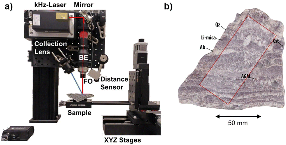

Fig. 1 (a) kHz μLIBS experimental set-up, showing the main components (BE: Beam Expander, FO: Focusing Objective). The red line represents the laser beam path, while the blue line represents the plasma light collection path. The optical fiber and the spectrometer are not represented in the image. (b) Photograph of the Li-mineralized aplite–pegmatite sample from the Fregeneda–Almendra field, with the sampling region shown in red. Note alternation of purple lepidolite-rich (Li-mica) and white albite-rich (Ab) layers; together with cassiterite (Cst), quartz (Qz) and amblygonite-group minerals (AGM).

The sample is placed on a set of XYZ linear motorized stages (Physik Instrumente (PI), Germany, with 200 mm, 150 mm, and 100 mm of travel range respectively) to precisely displace the sample during the analysis. These stages, together with a laser sensor for distance measurement, are used to control the lens-to-sample distance, allowing us to precisely control the sample positioning on the set-up, including the capability of re-analyzing a sample surface with an x–y–z reproducibility better than 1 μm. The elemental images presented in this work were recorded with a lateral resolution (i.e., shot-to-shot distance) of 17.5 μm and a typical crater diameter in the range of 10 μm. An argon flow (0.3 l min⁻¹) is introduced in the plasma to enhance the recorded signal.

The images are composed of 10 000 000 pixels (sequence of 5000 × 2000) with one spectrum measured for each single laser pulse at each spatial position of the sample (i.e., pixel). The sampling region covers an area of 30.6 cm². Through the use of a kHz laser, the entire sampling area was imaged in about 3 h per spectral region.

The spectral regions were selected based on the potential presence of emission lines from the elements of interest, which were identified in similar samples originating from the same region.^37,38 The reduced size of such a detector (sCMOS), combined with the required spectral resolution, imposes a reduced spectral range of analysis (∼40 nm for the 1200 lines per mm grating). Nevertheless, the low volume ablated in this LIBS configuration allows easily reproducing the analysis in order to cover the spectral range of interest. Four spectral regions were measured sequentially, three in the UV region, i.e., 241–281 nm; 280–319 nm; 320–358 nm, with 1200 lines per mm grating, and one in the VIS-IR spectral region, 662–824 nm with 300 lines per mm grating. After each imaging, we change the spectral region, and the sample returns to the starting point to restart the analysis. It is, therefore, possible that a slight difference between mappings can be observed for small minerals. The spectra were acquired with an integration time of 5 μs without any delay time.

Geological aspect and sample

Often referred to as the “new gasoline”, lithium plays a significant role in the current transformation driven by national and supranational entities towards a greener world. This transition is exemplified by the European Union's initiative to reduce the combustion engines from the vehicle fleet. Li is still the lightest of the known metals with the best energy/weight balance, making it perfect to be used in batteries. The world's largest known reserves occur as brines in low-grade evaporitic-type deposits, mainly concentrated within the “Lithium Triangle” a region encompassing parts of Bolivia, Chile, and Argentina. However, most of the “hard-rock “Li resources are represented by aluminosilicate phases disseminated within rare-metal granites and pegmatites.^39–41 Pegmatites of the Li–Cs–Ta (LCT) family that are not only enriched in economic concentrations of Li, but also in other critical metals such as Ta, Nb, Be, and Sn, are widespread and documented in several orogenic belts over the globe.^42,43 In pegmatites, spodumene is the main ore mineral used to produce Li-carbonates, although other Li-rich phases, such as petalite, lepidolite, and amblygonite-group minerals, represent significant resources.

Several occurrences of Li-enriched igneous rocks are reported in the Central Iberian Zone (CIZ) of the Iberian Massif (Spain and Portugal). They mainly consist of LCT aplite–pegmatite bodies clustering as dyke fields, or peraluminous rare-metal leucogranite stocks and cupolas, emplaced at the end of the Variscan orogeny during the late Carboniferous from ca. 320 to 300 Ma (millions of years ago).^44,45 The east-west-orientated 30 km long and 7 km wide Fregeneda–Almendra (FA) pegmatite field of the CIZ is located at the boundary between Spain and Portugal. This field comprises more than 100 (aplite-)pegmatite bodies and represents a typical expression of Iberian rare-metal magmatism. It is the host of various pegmatite types, notably Li-mineralized intrusions including petalite-, spodumene- and/or Li-mica (lepidolite)-bearing dykes mainly emplaced between ca. 315 and 308 Ma in Neoproterozoic to Cambrian metasedimentary rocks.^37,38,46 In addition to Li-aluminosilicates and common granitic minerals (quartz, albite ± K-feldspar ± muscovite ± apatite), Li-mineralized dykes commonly host Fe–Mn and Li–Al–F (amblygonite-group mineral: AGM) phosphates along with Sn (cassiterite) and Nb–Ta–Mn–Fe (CGM: columbite-group minerals) oxide minerals. Topaz and pyrochlore-group minerals (fluorcalciomicrolite) were rarely documented.

The investigated rock slab (Almendra) corresponds to the sample P010 of Ballouard et al.³⁸ (Fig. 2b in ref. 38; 41°0′N, 6°50′W), represented in Fig. 1b. It was collected from an aplite–pegmatite body that was emplaced in the north-eastern part of the FA pegmatite field and mostly consists of quartz, albite, Li-micas (Li-muscovite to lepidolite composition), muscovite, AGM, cassiterite, CGM and apatite. This sample is characterized by unidirectional solidification textures marked by the alternation Li-mica-rich and quartz-albite-rich millimeter to centimeter-thick zones with the long axis of crystals generally oriented perpendicular to the layering. The entire sample has a surface of 83 cm², while the sampling region covers an area of 30.6 cm² with a dimension of 5000 × 2000 pixels.

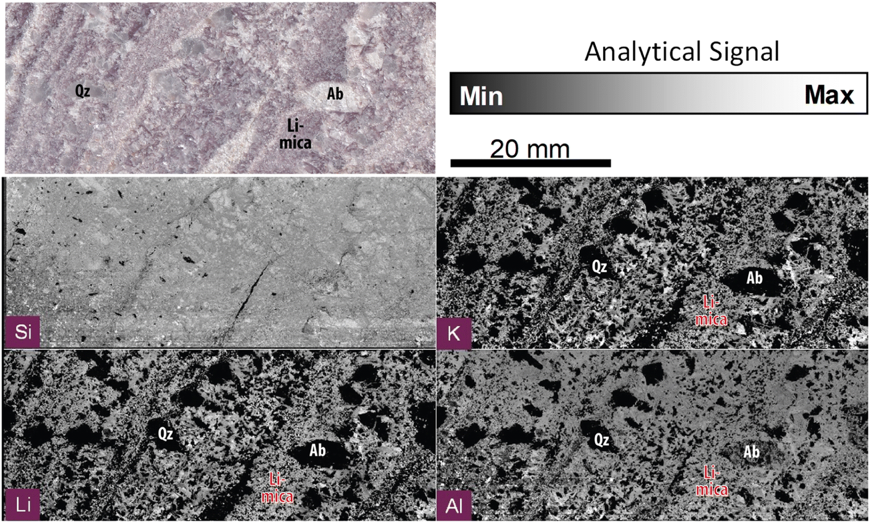Fig. 2 Compositional imaging using the analytical signal for the emission lines of Si I_{288 nm}, K I_{766 nm}, Li I_{670 nm} and Al I_{308 nm}, and the optical picture of the Almendra's sample.

Data treatment

The four datasets, one for each spectral range, result in a total of 40 million spectra, with a combined storage requirement of 200 GB, making the data treatment also challenging in terms of computational processing power. The first step of the data treatment workflow was to extract the emission lines' net area (after background subtraction) for all identified elements. Table 1 in the ESI† lists 34 elements identified in the sample with the emission lines taken as characteristic signatures for each of them. When various emission lines for the same element were available, the imaging map was reconstructed using the line with the highest intensity free from spectral interferences.

The elemental mapping of the Almendra sample, predominantly consisting of aluminosilicates with variable Li contents, may lead to misinterpretations of elemental abundance across different mineral phases. This is due to the matrix effect on the emission signal correlating with elemental composition. As a clear example, the Si signal presents a counterintuitive lower intensity in the areas identified as quartz (a pure siliceous phase SiO₂). Consequently, in this work, we propose to use an approach based on the presence/absence of specific elements to determine the mineralogical composition, transforming the intensity scale into binary values. An element is absent if its intensity falls below the threshold used to reconstruct the elemental binary mask, as explained in the following paragraph.

After adjusting the image's contrast, we create elemental binary masks. i.e., we transform the analytical signals recorded by the sCMOS (0–2¹⁶ counts) into binary (0/1) values, representing the presence or absence of one element at one specific pixel. This step excludes the elemental maps with possible atmospheric interferences (e.g., Ar, O, C) and those exhibiting sparse data points (e.g., Th, La). As explained in subsequent paragraphs, elemental masks, rather than gray-scale images, aim to simplify the process of identification of mineral phases. The masks' threshold was calculated using two different well-established methods for image thresholding. Otsu's method and the adaptive thresholding method. Both approaches were implemented by using the native Matlab R2022b functions. Otsu's thresholding method provides an optimal threshold by minimizing the within-class variance of the image pixels. Five levels were selected as they provide an appropriate threshold on maps with heterogeneously distributed intensity; whereas the adaptive thresholding method calculates different thresholds for smaller regions of an image, being useful for establishing the threshold value in smaller structures. Utilizing this dual approach enables us to identify elements' presence on the sample surface by fixing a threshold value for the analytical signal recorded, which is used to build the binary masks and minimize the influence of their distribution (in)homogeneity. Furthermore, we applied a median filter followed by close and open operations on the image to reduce the “salt-and-pepper” noise and smooth the edges (disk-shaped structuring element with radius 2). Once the elemental masks are defined, we define an assemblage of logic conditions about the presence (mandatory elements), absence (forbidden elements), or inconsequential (without influence on the decision). The comprehensive list of elements and their correlation with the mineral phases is presented in Table 1 – Results and discussion section. The selection of these elements was based, on one hand, on their presence in the expected mineral phases, considering previous petro-geochemical studies on Li-pegmatites from the FA pegmatite field, including the Almendra sample, and on the other hand, on their detectability using LIBS together with their presence in the sample (for instance, F was not considered due to its unclear detection using this method). Through logical operators such as AND, OR, and NOT, we integrate these elemental masks to accurately identify the mineral phases present in the sample according to their expected elemental composition.

Table 1 Elements required for the presence/possible/absence matrix and the percentage of pixels (number of pixels with respect to the total) attributed to each mineral phase identified

Mineral	Presence	Possible	Never	Abbreviation	Formula	Percent (%)
Quartz	Si	—	Li, P, Be, Sn Nb, Zr	Qtz	SiO2	35.83
Li-micas	K, Li	Al, Si	P, Be, Sn Nb, Fe, Zr	Lpd	K(Li; Al)3(Si; Al)4O10(F; OH)2	35.51
Feldspars + muscovite	Al, Si	K, Na, Ca	Li, P, Be, Sn Nb, Zr	Ab (albite)	NaAlSi3O8	12.91
				Kfs + Ms (K-feldspar + muscovite)	KAlSi3O8 + KAl2(Si3Al)O10(OH; F)2	11.54
Amblygonite	Al, P	Li, Na	Be, Sn, Nb Zr	AGM (amblygonite-group mineral)	(Li,Na)Al(PO4)(OH,F) + LiAl(PO4)(F,OH)	1.1
Al-phosphate	Al, P	—	Li
Cassiterite	Sn	—	—	Cst	SnO2	0.71
Beryl	Be, Si, Al		Nb	Brl	Be3Al2Si6O18	0.52
Other phosphates	P	—	Al, Li	Oth. Phos.		0.17
Fe-cookeite	Al, Si, Li, Fe	—	P, Be, Sn, Zr	Fe Cok.	LiAl4(Si3Al)O10(OH)8	0.14
Zircon	Si, Zr	—	Be, Sn, Nb	Zrn	ZrSiO4	0.07
Nb–Ta oxides	—	Nb Ta	—	CGM (columbite-group mineral)	(Mn,Fe)(Nb,Ta)2O6	0.05
Be-rich phase	Be	—	Si Nb	Be rich		0.02
Spodumene + petalite	Al, Si	Li, Na	K P Be	Spd + Ptl	LiAlSi2O6 + LiAlSi4O10	0.01
Apatite	Ca, P	—	Al Si Li P Be	Ap	Ca5(PO4)3(F,Cl,OH)	0.01
Holes	—	—	all	—	—	0.64
Mixed	>8	—	—	Mix.		0.03
Non assig.	—	—	—	N.A.		0.66

---

The data treatments were carried out using different tools: LasMap, a homemade data processing tool developed at Institut Lumière Matière-iLM, Lyon, France to specifically process LIBS spectra for imaging applications, Matlab R2022b (MathWorks, Inc.) for the mask creation and data treatment, and Fiji – ImageJ⁴⁷ for the image representation and treatment.

Results and discussion

The elemental images were based on representing the elements' analytical signal (net area of the emission lines⁴⁸) with respect to their XY spatial coordinates. The following elemental images comprise 10 000 000 pixels, one of the largest LIBS images ever produced. Fig. 2 illustrates our system's capability by reconstructing an image with some of the most abundant elements in our sample, Si, K, Al, and Li. Fig. 1SP (ESI)† presents a larger set of elemental maps. In this case, the term “abundant” refers to the spatial distribution of the elements, rather than the bulk concentration of each element in the sample, since elements such as F, which are expected to be present in large areas of the sample due to their geochemical traits, are not detectable due to their typically low sensitivity in LIBS. The Si, K, Al and Li elemental distribution maps are consistent with Almendra's expected mineralogy and allow efficiently distinguishing between the main rock-forming minerals, including quartz (Si), albite (Si, Al) and micas (Si, Al, K ± Li).

In addition to Li-phases, elemental mapping allows highlighting the presence of minerals enriched in Be, Sn, Nb, and Ta, and the sub-millimetric resolutions make it possible to discern regions where these elements manifest as pure phases or in mixed states (Fig. 3). The four pixels of interest of Fig. 3a along with corresponding spectra allow illustrating the different modes of occurrences of those elements. The simultaneous contribution of Nb and Ta likely reflecting the presence of CGM is illustrated by Pixel 01. Tin is found either alone, corresponding to cassiterite (Pixel 03), or associated with Nb for Pixel 02. The latter may reflect the occurrence of Nb-rich cassiterite, or the presence of cassiterite hosting small inclusions of CGM ranging from ca. 1 to 10 micrometers, as commonly documented in FA pegmatites.³⁸ The pixel 04 highlights the occurrence of a Be-rich mineral possibly corresponding to beryl (Be₃Al₂(Si₆O₁₈)).

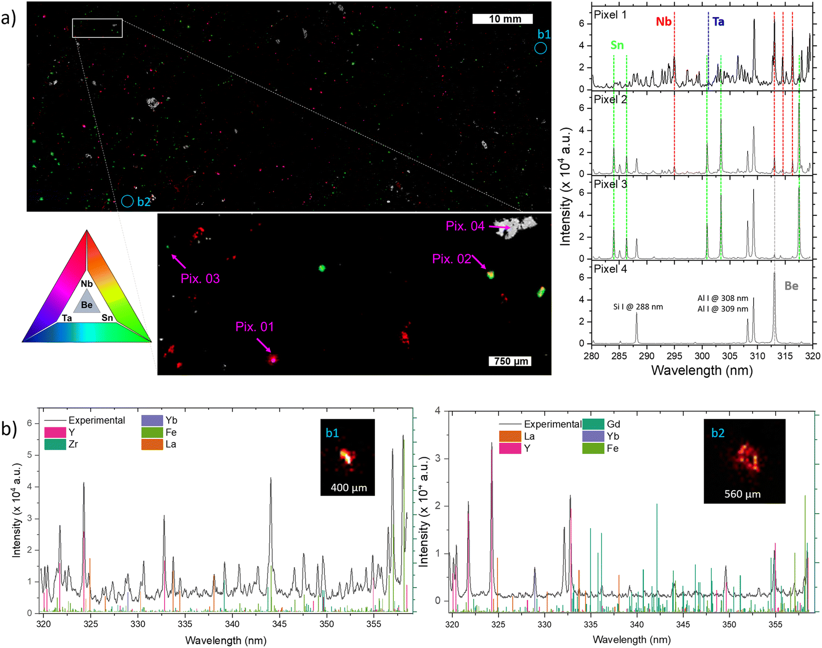Fig. 3 (a – Left) Nb (Red)–Sn (Green)–Ta (Blue)–Be (Gray) composite maps, representing the analytical signal of the emission lines Nb I @ 358 nm; Sn I @ 283 nm; Ta II @ 282 nm and Be II @ 313 nm. (a – Right) Spectra for the 4 pixels represented on the zoomed composite map. The dotted line color points to the emission line following the same RGB-Gr color legend. (b) Compositional maps for Yb II_{328 nm} showing zoomed regions for 2 REE-containing particles. The spectra show the experimental LIBS spectra (black) and simulated line intensity (Kurutz database, T = 7000 K, n_e = 10¹⁷ cm⁻³).

The imaging system's resolution (i.e., the pitch between measurements), around 17 micrometers, improves the identification of elements that might remain undetected with lower resolutions. Fig. 3b represents the extreme case where the elements are present in microscopic regions with dimensions of a few pixels. This is particularly evident with certain rare earth elements such as La, Yb, and Y, which were found as diminutive particles within the vast area of the 10 000 000 pixels image. These regions, possibly corresponding to monazite (La), xenotime (Y) or zircon (Yb), have submillimeter size, with a few pixels in diameter. Although not the main focus of this study, their presence highlights the potential of our high-resolution kHz LIBS imaging system to detect and analyze unforeseen elements across a large sampling area.

Mineral phase distribution

To reconstruct the mineralogical distribution of the investigated aplite–pegmatite sample we defined a set of logical operators regarding the presence/absence of specific elements, allowing us to identify the different mineral phases. The list of possible minerals was pre-defined based on previous mineralogical work on Li-pegmatite systems, including the FA pegmatite field and the investigated sample.

We consider binary values (masks) instead of the elemental intensity values for the mineral phase identification. The bibliography shows different approaches for identifying minerals based on different chemometrics or deep learning approaches.^22,49 However, in this case, the size of our dataset and the lack of reference samples for the training step render the use of these approaches challenging. Furthermore, the image-mask-based approach reduces the computation time for data treatment compared with other chemometrics multivariate alternatives. The mineral phase identification procedure follows the pipeline explained in the Data treatment section. Table 1 shows the investigated sample's possible mineral phases and the list of elements whose presence or absence is required during the mineral identification procedure. Highlighting the adaptability of our approach, we have introduced a novel category to accommodate potential elemental substitutions within the expected mineral compositions. For instance, in the case of Li-micas of the Li-muscovite to lepidolite series, the increase of the lepidolite end-member proportion is marked by the progressive replacement of tetrahedral Al by tetrahedral Si (e.g. Tischendorf et al.⁵⁰). Consequently, we consider the presence of any of both, while the simultaneous presence of K and Li is imperative to identify a given mineral as Li-mica. The last column of Table 1 displays the percentage of pixels attributed to each mineral phase based on the previously explained process. Furthermore, mixed phases (more than 8 elements identified) together with “holes” (no elements present) were identified.

Due to the size of some mineral phases being smaller than the crater size (10 μm), one pixel may be attributed to more than one mineral phase. Furthermore, we have based our approach on their ideal composition, although some substitutions of traces and minor components may have occurred (e.g., Sn and Nb incorporation in CGM and cassiterite, respectively). In addition, the different members of the same mineral group, such as AGM with various amounts of Na or F, as well as possible alteration products of AGM with undetected amount of Li (i.e. attributed to altered AGM), remain indistinguishable.

We have determined three principal combinations for pixels representing multiple phases: feldspar-quartz, cassiterite – CGM and quartz-altered (presence of Si, Al and Mg) phases. In order to attribute to each pixel a unique mineral phase, we have refined our methodology by incorporating supervised classification algorithms when appropriate. We trained our classification model with those particular pixels corresponding to a unique mineral phase according to our previously established logical conditions. The classification model generated is thus applied to those pixels presenting multiple phases. To build a more robust database and reduce the influence of outliers, the spectra were averaged in groups of 500 spectra chosen randomly from the dataset.

Furthermore, we tested different classification models, i.e., KNN, logistic classification, tree classification, and SVM, providing comparable results. The independent variables used in the classification models were selected as the analytical signals for different elements (typically the major elements) for each one of the classifications performed. The tree classification demonstrated the lowest variation when different and randomly selected training sets were chosen (ESI Fig. SP2†). Based on this algorithm, feldspars change from 27.9 to 24.43%, cassiterite changes from 0.72 to 0.71%, CGM from 0.0511 to 0.0508%, and quartz from 60.48 to 35.83%. In the previous results, feldspars have been considered as a single class. The composition of the feldspars corresponds to a ternary system consisting of K-feldspars (KAlSi₃O₈), albite (NaAlSi₃O₈) and anorthite (CaAl₂Si₂O₈). However, as expected for such evolved granitic rock and documented for the FA pegmatite field,⁵¹ the absence of a Ca-dominant cluster in our sample led us to infer a predominance of K-feldspar and albite. Under this assumption, a k-means clustering algorithm of only 2 classes was used, associated with K-feldspar or albite as a function of the mean signal of K and Na for the spectra of each cluster. Unfortunately, it was not possible to further discriminate between K-feldspar and muscovite, so they remained as a single class. Finally, it was possible to reconstruct the map of mineralogical phases of the sample, as represented in Fig. 4, being able to identify the phase for more than 99% of the pixels.

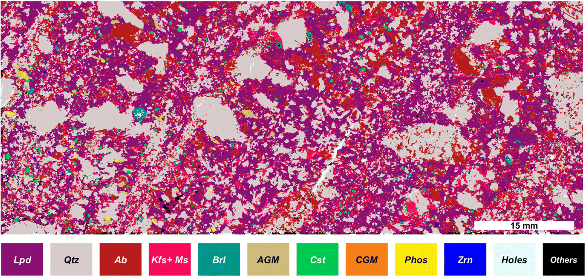Fig. 4 Mineralogical map based on selected mineral phase masks, for lepidolite, quartz, albite, K-feldspar + muscovite, beryl, amblygonite-group minerals, cassiterite, Nb–Ta oxides/columbite-group minerals, and zircon. In white are represented the regions without signal and other unidentified phases are shown in black. Each color corresponds to a single phase with a constant value (i.e., a binary mask), with no mixing between phases.

Lastly, we undertook a preliminary sample quantification based on its mineralogical composition. This is often referred to as “reverse normative calculation” or “inverse norm calculation.” The chemical composition of the original rock is revealed from the known minerals present in a rock, and knowing their respective volumes or weights in 2D distribution, along with their normative chemical compositions. The final bulk elemental composition is determined by summing up the proportionate contributions of each mineral, based on their respective normative stoichiometries. Note that our quantitative estimations inherently carry an elevated degree of uncertainty. However, even with these uncertainties, deriving an elemental composition from the mineralogical cartography of the sample is useful for certain applications. For instance, such an approach might be helpful in preliminary screening studies of potential ore samples, allowing for an estimation of a preliminary semi-quantitative elemental composition. In this regard, the following assumptions were made: (i) The 2D mineralogical distribution analyzed is considered representative of the bulk volume of the rock sample, (ii) the elemental composition of each mineral phase analyzed aligns with the normative one,⁵² and (iii) we have accurately identified the mineral phases in our sample.

Considering the three aforementioned hypotheses, it would be possible to estimate the number of elements in the sample, even if certain elements remain undetectable due to the sensitivity of the LIBS instrument. It is notably the case of F representing a major component of Li-micas, AGM and apatite.

The theoretical normative composition of minerals has no fixed value; thus, the actual composition in the Almendra sample may vary slightly. To determine the concentration range, we obtain the normative concentration of each mineral. Sometimes there is more than one value provided by the literature. In these cases, each mineral's composition is considered a discrete unit and the concentration ranges are calculated according to the combinations of each of these mineral phases. This approach led to the computation of all the possible combinations, resulting in 1728 possible combinations. Nevertheless, our methodology must pay special attention to those mineral phases whose elemental composition difference is indistinguishable for LIBS, significantly rendering them challenging to differentiate using our chosen method. Specifically, those compositions include AGM (i.e., montebrasite versus amblygonite), K-feldspar versus muscovite, and petalite versus spodumene. For these cases, we calculate the 13 824 (1728 × 8) possible combinations, i.e. we consider, for example, that in the sample, there are only K-feldspar, montebrasite and petalite, and no muscovite, amblygonite or spodumene and so on with all possible combinations, and the result is the range between the minimum and the maximum concentration values given in Table 2.

Table 2 Concentration range for the sample components based on the theoretical mineral phase components. The whole-rock compositions of two Li-mica-rich pegmatite samples from the Fregeneda–Almendra pegmatite field obtained from the literature are shown as reference values for preliminary comparison

	Reference values (wt%)		Estimated values (wt%)			Reference values (ppm)		Estimated values (ppm)
	Ref. 43	Ref. 37	Max	Min		Ref. 43	Ref. 37	Max	Min
SiO2	70.14	70.84	70.90	67.20	F	3700	3100	31 568	17 800
Al2O3	16.22	17.07	18.10	13.20	Li	2660	2600	8638	5425
Fe2O3	0.25	0.45	0.60	0	Be	203	208	242	187
MnO	0.07	0.03	0.40	0.20	Rb	1070	1080	1516	746
MgO	0.73	0.04	0.20	0	Nb	56	78.1	103	85
CaO	1.71	0.32	0.0	0	Ta	82	118	20	5
Na2O	5.51	6.3	2.00	1.40	Sn	350	768	1503	1502
K2O	2.12	2.15	5.60	4.40	Cs	236	379	655	16
TiO2	0.01	0.02	0.03	0.00
P2O5	0.68	0.82	0.56	0.56

---

While the results presented offer valuable quantitative insights into the bulk sample, quantitative chemical maps cannot be retrieved directly from LIBS imaging applications. Nonetheless, the capacity to analyze large sampling areas ensures that these rough estimates should serve as a foundation for initial investigations and screening studies. The lithium contents are significantly higher than those reported in the literature, exhibiting a factor of 3 to 4 times the reference value (2660 ppm). On one hand, the sensitivity of LIBS for lithium, with a detection limit on the order of parts per million (ppm), may lead to the misidentification of lithium-bearing minerals. On the other hand, even if we cannot discard an overestimation of the presence of lithium-bearing minerals, it is likely that our sample is actually richer in Li than literature samples, as it contains a significant percentage of Li-micas and AGM. Li concentrations up to ∼10 000 ppm have been documented in similar Li-mica-rich pegmatite samples from the Iberian Massif.⁴⁵

Implications and conclusions

This work demonstrates the capability of creating compositional maps of geological samples using μLIBS in the kHz regime. It combines the ability to measure large sample areas (tens of cm²) in a short amount of time, along with maintaining a lateral resolution on the order of a few micrometers. As a result of these characteristics, this work introduces one of the largest LIBS compositional images in the literature, acquired with a resolution lower than 20 μm, comprising 10 000 000 pixels (5000 × 2000).

Furthermore, thanks to the combination of improved spatial resolution and sampled area, it is possible to detect the presence of elements in tiny regions of interest at the microscale level, with very few pixels in size. This capability allows for the identification of small mineral phases whose element concentrations in the bulk sample are usually insignificant and would not be detectable under bulk LIBS analysis (mean LIBS spectrum). However, as these elements are highly concentrated in these tiny regions of interest, their detection is straightforward, making our system's high lateral resolution a key factor.

Utilizing elementary images of several millions of pixels, we have devised a methodology enabling the identification of mineral phases via uncomplicated mask-creation operations and logical relationships. Combining two masks, we have reconstructed the mineralogical map of a typical aplite–pegmatite Li-ore from the west-European Variscan belt. Lastly, an alternative approach is presented for the quantitative determination of these mineral phases and their theoretical composition. Notably, we have identified 14 different mineral phases in the investigated Fregeneda–Almendra aplite–pegmatite sample, including some phases with high economic interest, bearing Li (lepidolite, amblygonite-group minerals), Be (beryl and unidentified Be-rich phases), Sn (cassiterite), and Nb–Ta (columbite-group minerals). In addition, we have proved our capability of locating microscopic grains with possible geological interests, such as the presence of REE-bearing minerals (possibly xenotime((Y,Yb)PO₄) or monazite ((Ce,La,Nd,Th)PO₄) phases).

In conclusion, the use of kHz LIBS systems represents a significant advance in the field of applications of LIBS techniques, especially for elemental and phase imaging applications and, more specifically, for geological applications. It provides unique petro-geochemical information that can significantly contribute to a fast-comprehensive geological characterization and the definition of petrogenetic models, particularly in the framework of a system with light elements (Li, Be) in significantly heterogeneous rocks. This technique combines multi-elemental detection with spatial representation and allows both macro- and micro-scale analysis with simple, fast, and automated data processing.

There are no intrinsic limitations to consider images of tens or even hundreds of millions of spectra, which may be required for high-throughput analysis. Such datasets represent a current challenge in terms of multivariate processing. In this paper, we have considered univariate methods, looking for alternatives to solve our specific problem; however, the trend in traditional LIBS is using multivariate chemometric tools, which do not apply to these datasets using conventional computers. Ultimately, acquiring tens or hundreds of millions of spectra, resulting in a substantial volume of LIBS data within a few days, can significantly enhance the implementation of emerging deep-learning trends across various scientific disciplines.

Author contributions

Conceptualization: CALL, AT, CF, VMR. Data curation and software: CALL, AT, VMR. Formal analysis: CALL. Funding acquisition and resources: CD, VMR. Investigation: CALL, AT, CB. Methodology: CALL, CF, VMR. Project administration: CD. Supervision: VMR, CD. Writing – original draft: CALL, CB, CF. Writing – review & editing: All the authors.

Conflicts of interest

There are no conflicts to declare.

Acknowledgements

This work was supported by the French government “France 2030” initiative, under the DIADEM program managed by the “Agence Nationale de la Recherche” (ANR-22-PEXD-0014, “Libelul”) and the French Government “Plan de Relance”. Additional funding was provided by the ANR TRANSFAIR (ANR-21-CE01-0022-01), ANR-10-LABX-21-RESSOURCES21 and ERA-MIN/0001/2017–LIGHTS projects. In addition, we gratefully acknowledge Florian Trichard from ABLATOM S.A.S., Jean Michel Laurent, Shayne Harrel, and Antoine Varagnat from Andor Technologies, and Elena Vasileva and Håkan Karlsson from Hübner Photonics for fruitful discussions.

References

1. C. Fabre, Spectrochim. Acta, Part B, 2020, 166, 105799.
2. R. Harmon, C. Lawley and J. Watts, et al. , Minerals, 2019, 9, 718.
3. D. Chew, K. Drost, J. H. Marsh and J. A. Petrus, Chem. Geol., 2021, 559, 119917.
4. C. Fabre, K. Trebus and A. Tarantola, et al. , Spectrochim. Acta, Part B, 2022, 194, 106470.
5. J. Rakovský, P. Čermák, O. Musset and P. Veis, Spectrochim. Acta, Part B, 2014, 101, 269–287.
6. R. R. Hark and R. S. Harmon, in Laser-Induced Breakdown Spectroscopy, ed. S. Musazzi and U. Perini, Springer Berlin Heidelberg, Berlin, Heidelberg, 2014, vol. 182, pp. 309–348.
7. C. Alvarez-Llamas, C. Roux and O. Musset, Spectrochim. Acta, Part B, 2018, 148, 118–128.
8. M. T. Sweetapple and S. Tassios, Am. Mineral., 2015, 100, 2141–2151.
9. B. Lemière and R. S. Harmon, in Portable Spectroscopy and Spectrometry, John Wiley & Sons, Ltd, 2021, pp. 455–497.
10. C. Fabre, N. E. Ourti, C. Ballouard, J. Mercadier and J. Cauzid, J. Geochem. Explor., 2022, 236, 106979.
11. V. Balaram and S. S. Sawant, Minerals, 2022, 12, 394.
12. A. K. Knight, N. L. Scherbarth, D. A. Cremers and M. J. Ferris, Appl. Spectrosc., 2000, 54, 331–340.
13. R. C. Wiens, S. Maurice and B. Barraclough, et al. , Space Sci. Rev., 2012, 170, 167–227.
14. S. Maurice, R. C. Wiens and P. Bernardi, et al. , Space Sci. Rev., 2021, 217, 47.
15. R. R. Hark and L. J. East, in Laser-Induced Breakdown Spectroscopy: Theory and Applications, ed. S. Musazzi and U. Perini, Springer, Berlin, Heidelberg, 2014, pp. 377–420.
16. B. Busser, S. Moncayo and J.-L. Coll, et al. , Coord. Chem. Rev., 2018, 358, 70–79.
17. C. Fabre, D. Devismes and S. Moncayo, et al. , J. Anal. At. Spectrom., 2018, 33, 1345–1353.
18. J.-M. Baele, H. Bouzahzah and S. Papier, et al. , Geol. Belg., 2021, 24, 125–136.
19. J. D. Pedarnig, S. Trautner and S. Grünberger, et al. , Appl. Sci., 2021, 11, 9274.
20. V. Gardette, V. Motto-Ros and C. Alvarez-Llamas, et al. , Anal. Chem., 2023, 95, 49–69.
21. K. Rifai, F. Doucet, L. Özcan and F. Vidal, Spectrochim. Acta, Part B, 2018, 150, 43–48.
22. K. Rifai and M.-C. Michaud Paradis, et al. , Minerals, 2020, 10, 918.
23. V. Motto-Ros, S. Moncayo, C. Fabre and B. Busser, in Laser-Induced Breakdown Spectroscopy, Elsevier, 2020, pp. 329–346.
24. K. Novotný, J. Kaiser and M. Galiová, et al. , Spectrochim. Acta, Part B, 2008, 63, 1139–1144.
25. J. Klus, P. Mikysek and D. Prochazka, et al. , Spectrochim. Acta, Part B, 2016, 123, 143–149.
26. A. Limbeck, L. Brunnbauer and H. Lohninger, et al. , Anal. Chim. Acta, 2021, 1147, 72–98.
27. C. Méndez-López, L. Javier Fernández-Menéndez and C. González-Gago, et al. , Opt Laser. Technol., 2023, 164, 109536.
28. C. Alvarez-Llamas, J. Pisonero and N. Bordel, Spectrochim. Acta, Part B, 2016, 123, 157–162.
29. S. Müller and J. A. Meima, Spectrochim. Acta, Part B, 2022, 189, 106370.
30. S. Müller, J. A. Meima and H.-E. Gäbler, J. Geochem. Explor., 2023, 250, 107235.
31. R. Noll, H. Bette, A. Brysch, M. Kraushaar, I. Mönch, L. Peter and V. Sturm, Spectrochim. Acta, Part B, 2001, 56, 637–649.
32. D. Diaz and D. W. Hahn, Spectrochim. Acta, Part B, 2020, 166, 105795.
33. F.-A. Barreda, C. Nicolas and J.-B. Sirven, et al. , Sci. Rep., 2015, 5, 15696.
34. H. Bette and R. Noll, J. Phys. D: Appl. Phys., 2004, 37, 1281–1288.
35. F. Boué-Bigne, Appl. Spectrosc., 2007, 61, 333–337.
36. M.-C. M. Paradis, F. R. Doucet, K. Rifai and L. Ç. Özcan, et al. , Minerals, 2021, 11, 859.
37. E. Roda-Robles, R. Vieira and A. Lima, et al. , Lithos, 2023, 452–453, 107195.
38. C. Ballouard, P. Carr and F. Parisot, et al. , BSGF Earth Sci. Bull., 2024, 195, 3.
39. B. Gourcerol, E. Gloaguen and J. Melleton, et al. , Ore Geol. Rev., 2019, 109, 494–519.
40. T. Bibienne, J.-F. Magnan, A. Rupp and N. Laroche, Elements, 2020, 16, 265–270.
41. R. J. Bowell, L. Lagos, C. R. de los Hoyos and J. Declercq, Elements, 2020, 16, 259–264.
42. P. Cerny, D. London and M. Novak, Elements, 2012, 8, 289–294.
43. R. L. Linnen, M. Van Lichtervelde and P. Cerny, Elements, 2012, 8, 275–280.
44. S. E. Kesler, P. W. Gruber and P. A. Medina, et al. , Ore Geol. Rev., 2012, 48, 55–69.
45. E. Roda-Robles, C. Villaseca and A. Pesquera, et al. , Ore Geol. Rev., 2018, 95, 408–430.
46. J. Errandonea-Martin and I. Garate-Olave, et al. , Ore Geol. Rev., 2022, 150, 105155.
47. J. Schindelin, I. Arganda-Carreras and E. Frise, et al. , Nat. Methods, 2012, 9, 676–682.
48. V. Motto-Ros, S. Moncayo, F. Trichard and F. Pelascini, Spectrochim. Acta, Part B, 2019, 155, 127–133.
49. N. Herreyre, A. Cormier and S. Hermelin, et al. , J. Anal. At. Spectrom., 2023, 38, 730–741.
50. G. Tischendorf, B. Gottesmann, H.-J. Förster and R. B. Trumbull, Mineral. Mag., 1997, 61, 809–834.
51. E. Roda Robles, A. Pesquera Perez, F. Velasco Roldan and F. Fontan, Mineral. Mag., 1999, 63, 535–558.
52. Handbook of Mineralogy, ed. J. W. Anthony, R. A. Bideaux, et al., Mineralogical Society of America, 2003, http://www.handbookofmineralogy.org/.

---

Footnote

† Electronic supplementary information (ESI) available. See DOI: https://doi.org/10.1039/d3ja00438d

---