
 Open Access Article
 This Open Access Article is licensed under a
 Creative Commons Attribution 3.0 Unported Licence
Two decades of changing anthropogenic mercury emissions in Australia: inventory development, trends, and atmospheric implications†
Stephen
MacFarlane
a,
Jenny A.
Fisher
 *a,
Hannah M.
Horowitz
b and
Viral
Shah
c
*a,
Hannah M.
Horowitz
b and
Viral
Shah
c
aCentre for Atmospheric Chemistry, School of Earth, Atmospheric and Life Sciences, University of Wollongong, Wollongong, NSW, Australia. E-mail: jennyf@uow.edu.au
bDepartment of Civil and Environmental Engineering, University of Illinois at Urbana-Champaign, Urbana, IL, USA
cHarvard John A. Paulson School of Engineering and Applied Sciences, Harvard University, Cambridge, MA, USA
First published on 23rd May 2022
Abstract
Mercury is a toxic environmental pollutant emitted into the atmosphere by both natural and anthropogenic sources. In Australia, previous estimates of anthropogenic mercury emissions differ by up to a factor of three, with existing inventories either outdated or inaccurate and several lacking Australia-specific input data. Here, we develop a twenty-year inventory of Australian anthropogenic mercury emissions spanning 2000–2019 with annual resolution. Our inventory uses Australia-specific data where possible and incorporates processes not included in other Australian inventories, such as delayed release effects from waste emissions. We show that Australian anthropogenic mercury emissions have decreased by more than a factor of two over the past twenty years, with the largest decrease from the gold production sector followed by brown coal-fired power plants and commercial product waste. Only the aluminium sector has shown a notable increase in mercury emissions. Using a global 3-D chemical transport model (GEOS-Chem), we show that the reduction in emissions has led to a small decrease in mercury deposition to the Australian continent, with annual oxidised mercury deposition ∼3–4% lower with present day emissions than with emissions from the year 2000. We also find that Australian emissions are not accurately represented in recent global emissions inventories and that differences between inventories have a larger impact than emissions trends on simulated mercury deposition. Overall, this work suggests a significant benefit to Australia from the Minamata Convention, with further reductions to Australian mercury deposition expected from decreases in both Australian and global anthropogenic emissions.
Environmental significanceAnthropogenic mercury emissions to the atmosphere are the most readily controlled driver of mercury pollution, with subsequent impact on the global mercury cycle. This work investigates anthropogenic mercury emissions in Australia, the 136th country to ratify the Minamata Convention on Mercury. We show how a combination of industry-driven technology upgrades, power plant closures, and other factors have led to a steep decline in mercury emissions over the past two decades. Neither the magnitude nor the sectoral distribution of these emissions are accurately represented in the global emission inventories used in modelling studies. Our results highlight the benefit of using up-to-date, location-specific knowledge where possible when constructing anthropogenic emissions inventories for use in scientific and policy analyses. |
1 Introduction
Mercury is a highly toxic trace element, with both natural and anthropogenic sources, that poses significant hazards to the environment and to human health.1,2 Mercury emitted to the atmosphere can be transported significant distances as long-lived gaseous elemental mercury (Hg0) and deposited to ecosystems as both Hg0 and highly soluble oxidised mercury (HgII), eventually bioaccumulating in food webs in its methylated form.3,4 To protect against the detrimental effects of mercury, the Minamata Convention on Mercury, an international treaty, requires parties to reduce anthropogenic releases of mercury to the environment.5 In December 2021, Australia became the 136th party to ratify the Convention. There is now an urgent need to understand Australia's controllable mercury emissions to effectively comply with the terms of the Convention; however, there is currently no anthropogenic mercury emission inventory that is fit-for-purpose for modern-day Australia.6 Here, we develop a twenty-year inventory of Australian anthropogenic mercury emissions spanning 2000–2019 and use the new inventory to quantify sectoral trends in mercury emissions and to evaluate the implications for atmospheric mercury concentrations and deposition.Australia is responsible for a relatively small share of total global anthropogenic emissions but on a per capita basis has been estimated to have some of the highest emission rates in the world.7 Historically, the major sources of Australian anthropogenic mercury emissions have been industrial-scale metal production (mainly gold) and fossil fuel combustion in coal-fired power plants.8 In the past, gold production emissions derived almost exclusively from a single facility in Kalgoorlie, Western Australia,8 while combustion emissions derived from a mix of brown coal-fired power plants in Victoria and South Australia and black coal-fired power plants in New South Wales, Queensland, and Western Australia.9 Over the past two decades, both sectors have experienced substantial change. At the Kalgoorlie facility, technological upgrades have virtually eliminated mercury emissions.6 Meanwhile, a third of Australia's coal-fired power plants have closed in recent years, including one of the largest brown coal-fired power plants.10
These changes in the emissions landscape, coupled with uncertainties and inconsistencies in the calculation of mercury emissions from different sectors, have led to very large disparities in estimates of Australian anthropogenic mercury emissions. Fisher and Nelson6 compared Australian anthropogenic emission estimates from four global inventories7,11–13 and one national inventory8 and found estimates ranged from 7.7 to 27 Mg yr−1. Much of the difference stemmed from discrepancies in input datasets and methodologies. For example, most of the global inventories did not account for the low mercury content and high moisture content present in Australian coal,9 and in one case these errors were compounded by not including any mercury capture from air pollution control devices at Australian coal-fired power plants.6 The national-scale inventory produced by Nelson et al.8 made the best use of local knowledge and input data; however, the inventory was developed for 2006, before the changes in the gold production and power plant sectors outlined above. As a result, Fisher and Nelson6 concluded that none of the existing inventories are suitable for use in present-day Australia and none provide consistent and reliable estimates that can be used to track change over time.
An alternative national-scale estimate of Australian anthropogenic mercury emissions comes from the National Pollutant Inventory (NPI), an Australian emissions database where facilities self-report emissions on an annual basis. The NPI has the advantage of covering a long timeframe (since 1999), but there are inconsistencies caused by changes in reporting thresholds and methodologies that can lead to spurious emissions trends in the database. Further, the NPI has been found to substantially underestimate mercury emissions from brown coal-fired power plants9 and to have inconsistent or missing data for other sources such as crematoria.8,9 These considerations mean that the NPI alone cannot be considered an accurate representation of Australian anthropogenic mercury emissions and cannot be used for trend analysis.
A further point of difference between existing inventories is the treatment of waste emissions from disposal and breakage of mercury-containing products. Horowitz et al.14 previously showed that because many products are used for decades before disposal, mercury contained in these products is not emitted until 10–50 years after their production. Global historical consumption of mercury-containing commercial products peaked in the 1970s14 and has since declined sharply in developed countries. Because of the delayed disposal and associated mercury emission, the 1970s consumption peak continues to influence present-day mercury emissions from commercial products. Most existing inventories have ignored these historical trends and used present-day consumption data to estimate present-day disposal by assuming a one-to-one relationship between consumption and disposal.8,11 However, that assumption will underestimate waste mercury emissions by not accounting for the fact that products disposed of today contain more mercury than those produced today. Conversely, the few inventories that have included delayed emissions from consumer products12,15,16 have overestimated these emissions for Australia by not accounting for historical changes in global consumption patterns.6 The differences can be substantial, with waste emissions ranging from as little as 47 kg yr−1 to as much as 5.1 Mg yr−1.6 Meanwhile, the facility-based NPI inventory does not account for waste emissions at all.
In response to the lingering uncertainties in quantifying Australian mercury emissions, development of an updated, time-varying Australian anthropogenic emissions inventory has been identified as a critical research need.6 In this paper, we address that need. We combine mercury emission data from the NPI with improved estimates of mercury emissions from coal-fired power plants, cremation, and disposal of commercial products (accounting for delayed release) to quantify annually resolved, spatially distributed emissions from 2000 to 2019. We evaluate national-scale trends in sectoral and total anthropogenic emissions over the past two decades and then use these emissions as input to a global atmospheric mercury model to investigate the impact on regional atmospheric mercury concentration and deposition.
2 Methods
2.1 Development of the emission inventory
We constructed a new anthropogenic emissions inventory for Australia with annual resolution from 2000 to 2019. The inventory includes both point source and distributed emissions. Section 2.1.1 describes the point source emissions, derived largely from the NPI but with exceptions for coal-fired power plants. Section 2.1.2 describes the distributed emissions. Section 2.1.3 provides the speciation information, and Section 2.1.4 describes the uncertainties. The new inventory is open access and can be downloaded from https://doi.org/10.5281/zenodo.6383431.NPI data for each year were downloaded directly from the NPI website.17 The annual NPI data are provided on an Australian financial year basis (1 July to 30 June); in what follows, we refer to these emissions by the year in which they start (e.g., the reported 2000–2001 emissions are referred to as “2000 emissions”) to make the text more readable. Data in the NPI are reported by each facility that emits any of 93 specified pollutants to air, land or water, as mandated by the Australian National Environmental Protection Measure. For mercury, the mandatory reporting threshold is currently 5 kg yr−1 but was 10 Mg yr−1 until 2007. To avoid discontinuities in our inventory, we examined the NPI logs that record the year in which facilities were first added to the database for any significant emission sources added to the database between 2000 (when our inventory begins) and 2007 (when the threshold changed). The Gidji roaster, a single facility that once dominated Australia's anthropogenic emissions,8 has been operational since 1989 but was only added to the database in 2004. For earlier years, we estimated emissions from the Gidji facility using an emission rate of 1.08 kg h−1 measured during stack testing conducted by Kalgoorlie Consolidated Gold Mines Pty Ltd (KCGM).18 Following the same assumptions used by KCGM, we assumed the roaster was operating 75% of the time during these years. Our calculated emissions for the Gidji roaster in these earlier years (shown in Section 3) are within 10% of the reported emissions for 2004. Apart from the Gidji roaster, we found that none of the other facilities added to the NPI between 2000 and 2007 were major mercury emitters, with all added facilities combined accounting for less than 1% of total annual emissions. We therefore ignored emissions from these facilities in the years before they were added to the database.
For brown coal-fired power plants, Nelson9 found that the NPI substantially underestimates mercury emissions because when coal mercury contents are not known, facilities are allowed to estimate emissions using a generic mercury emission factor (1.6 × 10⁻⁶ kg per tonne at the time of their work9). By comparing the NPI-reported emission to a separate estimate based on coal consumption data and measured brown coal mercury contents, Nelson9 showed that the generic mercury emission factor in the NPI was much too low (by a factor of ∼20), overestimating mercury capture in air pollution control devices and underestimating emissions. In 2012, the NPI increased the generic emission factor to 2.6 × 10⁻⁵ kg per tonne.19 While use of the newer emission factor would lead to emission estimates that are better aligned with the consumption-based estimates of Nelson,9 the change to the reporting methodology causes inconsistencies in the NPI record between emissions reported before 2012 and those reported after.
We therefore did not use the NPI estimates for brown coal-fired power plants and instead calculate the emissions using the coal consumption-based method described by Nelson.9 Annual total Australian brown coal consumption was obtained from the Australian Energy Update 2020 (Table P)20 and multiplied by an assumed coal mercury content of 0.032 ppm based on extensive measurements from Australian brown coals21 and corrected for moisture content.9 This estimate was then corrected for mercury capture by electrostatic precipitator (ESP) air pollution control devices using an assumed mercury capture rate of 2% as recommended in the NPI Emission Estimation Technique Manual.19 Note that ESPs are the only air pollution control technology in use in Australian brown coal-fired power plants and are known to have relatively poor capture efficiencies for mercury from brown coals.8,11 Mercury emission factors and mercury capture rates used to estimate emissions for all non-NPI sectors are shown in Table 1.
| Sector | Emission factor | Reference |
|---|---|---|
| a Mercury emission factor is the product of assumed coal mercury contents of 0.032 ppm (from ref. 9) and assumed fraction of mercury emitted of 0.98 (from ref. 19). b Same as (a) but assuming coal mercury contents of 0.05 ppm (from ref. 9) and fraction of mercury emitted of 0.81 (from ref. 19). | ||
| Black coal | 3.14 × 10⁻⁵ kg per tonne | Footnotea |
| Brown coal | 4.05 × 10⁻⁵ kg per tonne | Footnoteb |
| Cremation | 1.55 × 10⁻³ kg per cremation | NPI24 |
![[thin space (1/6-em)]](https://www.rsc.org/images/entities/char_2009.gif) |
||
| Refined petroleum | ||
| LPG | 2.32 × 10⁻⁶ kg per tonne | Nelson et al.8 |
| Fuel oil | 0.67 × 10⁻⁶ kg per tonne | Nelson et al.8 |
| Gasoline | 1.00 × 10⁻⁶ kg per tonne | Nelson et al.8 |
| Diesel | 0.40 × 10⁻⁶ kg per tonne | Nelson et al.8 |
| Aviation fuel | 1.50 × 10⁻⁶ kg per tonne | Liang et al.,25 Wilhelm26 |
Total annual emissions from brown coal-fired power stations calculated as described above were then distributed amongst the eight power stations that were active at some point during the 2000–2019 inventory period. To do so, we used the distribution of carbon dioxide (CO2) emissions as a proxy for the distribution of mercury emissions, following Schofield et al.22 For each power plant in each year, we calculated the fractional contribution to CO2 emissions from all brown coal-fired power plants active in that year and applied that fraction to total annual mercury emissions from brown coal-fired power plants. CO2 emissions from each power plant were obtained from the Australian Clean Energy Regulator23 for every year from 2013 onwards. Prior to 2013, reliable CO2 emission data were unavailable, and so the CO2 fractions calculated for 2013 were used for all earlier years (we did not use a multi-year average, as several power plants closed between 2013 and 2019).
For black coal-fired power plants, Nelson9 previously found that the NPI did not suffer from the same biases as seen for brown coal-fired power plants. In that analysis, based on data for the year 2004, the NPI-reported emissions were consistent with the coal consumption-based estimate, assuming a mercury capture efficiency of 67%. The 67% capture rate used by Nelson9 was consistent with the NPI recommendations at the time (46% for ESPs and 83% for Fabric Filters, FFs), but these numbers were revised in 2012 to a much lower rate of 19% for both technologies.19 More recently, Garg et al.27 found that the NPI significantly underestimated mercury emissions from black coal-fired power plants in New South Wales relative to estimates based on electricity data.
For our analysis, we compared NPI-reported emissions to those calculated based on coal consumption (as used for brown coal-fired power plants) and found significant discrepancies, with the NPI estimates 20–300% lower. Trends from the NPI were also unreliable, with year-to-year inconsistencies caused by changes in reporting methods, including the change to the mercury capture rates and associated emission factors in 2012.19 We also compared both emission estimates to independent electricity generation data from black coal-fired power plants20 and found only the consumption-based estimate reproduced the interannual variability of the electricity data.
We therefore estimated emissions from black coal-fired power plants using the same method as used for brown coal-fired power plants. Annual total Australian black coal consumption was obtained from the Australian Energy Update 2020 (Table P)20 and multiplied by an assumed coal mercury content of 0.05 ppm based on measurements from 100 Australian black coal samples.9,28,29 This estimate was then corrected for mercury capture using the 19% mercury capture rate currently recommended in the NPI Emission Estimation Technique Manual.19 We then distributed the emissions amongst black coal-fired power plants using CO2 emissions as a proxy, as for the brown coal-fired power plant emissions.
Australian cremation emissions were estimated by combining the annual number of deaths from the Australian Bureau of Statistics31 with an assumed cremation rate of 67% (based on information from the Australasian Cemeteries & Crematoria Association8). We applied a mercury emission factor of 1.55 g Hg per cremation as specified in the NPI Emission Estimation Technique Manual.24 To the best of our knowledge, mercury capture devices are not used in Australian crematoria.32
For petroleum product emissions, we followed the methodology of Nelson et al.8 to relate emissions to consumption. No single consumption dataset was available for the full period, so we combined 2000–2010 data from the Australian Bureau of Agricultural and Resource Economics and Sciences33,34 with 2010–2020 data from the Australian Petroleum Statistics 2021.35 For the latter, we assumed equivalence between product sold and consumption, which resulted in consumption values that were on par with those from the earlier dataset. Volumetric consumption was converted to mass units using the following best estimates of petroleum product densities: 520 kg m−3 for liquified petroleum gas (LPG),36 750 kg m−3 for automotive gasoline,37 890 kg m−3 for diesel,37 886 kg m−3 for fuel oil,38 786 kg m−3 for aviation turbine fuel,39 and 715 kg m−3 for aviation gasoline.39 From the mercury content data compiled by Nelson et al.8,26,40,41 combined with aviation fuel data,25,26 we assumed mercury emission factors as shown in Table 1. We did not include any mercury emissions from consumption of natural gas as previous work has shown insignificant emissions due to mercury removal during recovery.42 Residential coal combustion is negligible in Australia11 and is therefore not included here.
A major improvement in our inventory over previous inventories is in the treatment of waste emissions from breakage and disposal of mercury-containing products. Unlike previous national-scale estimates,8 we account for delays between consumption and disposal (emission) for some products. We improve upon previous global estimates of delayed emission12,15,16 by better accounting for historical changes in Australia's share of consumption.
We initially attempted to estimate Australian product mercury emissions at annual resolution using United Nations (UN) import and export data as described by Nelson et al.8 However, we found the UN data unreliable, with significant data gaps and unexplained discontinuities (i.e., year-on-year changes of as much as a factor of 200) during our 2000–2019 study period. Given our focus here on decadal-scale change, use of these data would have introduced unacceptable spurious trends and interannual variability. We therefore opted to instead use a coarser resolution but more self-consistent methodology, initially described by Horowitz et al.14 A weakness of this method is that the underlying data are only available at decadal resolution. For our purposes, decadal-scale estimates are sufficient to understand the relative importance of emissions from the waste sector and the decadal-scale trends in these emissions. We acknowledge that the lack of annually resolved waste emissions is a limitation of our work.
Here we briefly describe our methodology; full details can be found in Appendix 1. Following Horowitz et al.,14 we first calculated product mercury consumption at decadal scale (2000, 2010, 2020) for four product categories: lamps, batteries, medical devices, and wiring and measuring devices (see Appendix 1 for details). The historical consumption data used here are only available at the regional (Oceania) rather than national (Australia) scale.
We first calculated total Oceania consumption. For lamps and batteries, we used previously compiled Oceania consumption data7,43,44 and extrapolated to 2020. For medical devices, we used developed world consumption data from Horowitz et al.,14 multiplied by the Oceania fraction derived in that work and extrapolated to 2020. For wiring and measuring devices, we started from the global and developed world consumption data from Horowitz et al.14 and calculated the Oceania fraction based on regional consumption data from other sources.7,43,44 In the absence of regional data for years earlier than 1990 (needed for the delayed emission calculations), we assumed Oceania accounted for the same fraction of consumption in earlier decades as it did in 1990. For all product categories, we derived Australian consumption from Oceania consumption using Gross Domestic Product at Purchasing Power Parity (GDP-PPP) from the World Bank45 to determine the fraction of Oceania consumption attributed to Australia (following AMAP/UNEP7).
We next used the estimated Australian consumption values to estimate disposal. Following Horowitz et al.,14 we assumed delayed (>10 year) disposal only for wiring and measuring devices. We applied the same delays as in Horowitz et al.:14 10% disposal 10 years after consumption, 40% disposal after 30 years, and 50% disposal after 50 years. For all other categories, product lifetimes are thought to be less than 10 years;46–49 therefore, at the decadal scale used at this stage, disposal was assumed to equal consumption. We tested the implications of this assumption and found the resulting difference in estimated waste emissions to be much less than the uncertainty (Section 2.1.4). More details of this test can be found in the ESI (Section S1 and Table S1†).
Next, we calculated mercury emission factors from disposal of mercury-containing products using the air distribution factors from Horowitz et al.,14 which account for both changes in disposal method (e.g., landfill versus incineration versus recycling) over time and different emission factors for each disposal method. For 2000 and 2010 emissions, we used the Horowitz et al.14 air distribution factors directly. For 2020, we extrapolated the Horowitz et al.14 air distribution factors for each disposal method and product to 2020.
Finally, we applied the decadal-scale, product-specific mercury emission factors to the decadal-scale, product-specific disposal estimates. We then interpolated these from decadal to annual scale and distributed spatially using population data, as described above.
| Sector | Hg0 | HgII(g) | HgP | Source |
|---|---|---|---|---|
| a Weighted average of speciation factors from FF and ESP plants, assuming a distribution of 57% FF and 43% ESP in Australian black coal-fired power plants.9 b Average of three cement plants measured by Wang et al.51 c Average anthropogenic Australian speciation calculated from speciation reported in Nelson et al.8 | ||||
| Black coala | 53.4 | 45.6 | 1.0 | Zhang et al.50 |
| Brown coal | 58.0 | 41.0 | 1.0 | Zhang et al.50 |
| Cementb | 23.8 | 75.7 | 0.5 | Wang et al.51 |
| Chlor-alkali | 70.0 | 30.0 | 0.0 | AMAP/UNEP52 |
| Copper | 50.0 | 50.0 | 0.0 | Zhang et al.50 |
| Cremation | 80.0 | 15.0 | 5.0 | AMAP/UNEP52 |
| Ferrous metals | 32.1 | 62.9 | 5.0 | Muntean et al.13 |
| Gold | 32.0 | 57.0 | 11.0 | Zhang et al.50 |
| Lead | 39.0 | 61.0 | 0.0 | Zhang et al.50 |
| Non-ferrous metals (Exc. Cu, Pb, Zn) | 80.0 | 15.0 | 5.0 | Zhang et al.50 |
| Oil refiningc | 77.0 | 17.0 | 6.0 | Nelson et al.8 |
| Other industryc | 77.0 | 17.0 | 6.0 | Nelson et al.8 |
| Refined petroleum products | 50.0 | 50.0 | 0.0 | AMAP/UNEP52 |
| Waste | 20 | 60 | 20 | AMAP/UNEP52 |
| Zinc | 55 | 44 | 1 | Zhang et al.50 |
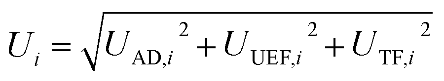 | (1) |
As an example, for coal-fired power plants, UAD,i is the uncertainty on the coal consumption data, UUEF,i is the uncertainty on the unabated emission factor from burning coal (from the coal mercury contents), and UTF,i is the uncertainty on the mercury capture from ESPs and/or FFs. We applied eqn (1) to all sectors except waste, for which we assumed an overall uncertainty of 300% as used in the GMA2018 Technical Background Report.11
In the absence of uncertainty estimates for the primary data sources used here, we took UAD,i and UUEF,i from the GMA2018 Technical Background Report. For UTF,i, the GMA2018 Technical Background Report sets uncertainty values that vary based on the overall efficiency of the mercury capture technology.11 For “low abatement” sectors with mercury capture rates of up to 30%, UTF,i was set to 40% (capped at 0, i.e., no mercury capture). UTF,i decreased to 20% for “medium abatement” sectors (mercury capture rates of 30–50%) and to 10% for “high abatement” sectors (mercury capture rates of 50–85%). No sectors in our study had mercury capture rates above 85%. To determine which abatement category to use for each sector, we used the average reduction efficiencies from the NPI Emission Estimation Technique Manual19 where possible and otherwise used the values from the GMA2018 Technical Background Report.11
Table 3 shows the values for UAD,i, UUEF,i, and UTF,i used here, along with the total uncertainty Ui for each sector. We include both a lower and upper bound for the total uncertainty to account for the fact that UTF,i is capped at 0% for low abatement sectors. For coal-fired power plants, our lower bound uncertainty is consistent with the ±30% uncertainty assumed by Nelson et al.8 for all industrial sectors (revised downward from their earlier work9).
| Sector | U AD | U UEF | U TF | U i – lower | U i – upper |
|---|---|---|---|---|---|
| a From Table A3.7.1 in ref. 11. b From Table A3.7.3 in ref. 11 capped at 0% for low abatement sectors: black and brown coal-fired power plants, cremation, oil refining, other industry, and waste. | |||||
| Black coal-fired power plants | 5 | 30 | 40 | 30 | 50 |
| Brown coal-fired power plants | 5 | 30 | 40 | 30 | 50 |
| Cement production | 5 | 50 | 20 | 54 | 54 |
| Chlor-alkali | 5 | 50 | 10 | 51 | 51 |
| Cremation | 5 | 50 | 40 | 50 | 64 |
| Gold production | 5 | 50 | 20 | 54 | 54 |
| Oil refining | 5 | 50 | 40 | 50 | 64 |
| Other industry | 5 | 50 | 40 | 50 | 64 |
| Other metal production | 5 | 50 | 10 | 51 | 51 |
| Refined petroleum products | 5 | 50 | 40 | 50 | 64 |
| Waste | — | — | — | 300 | 300 |
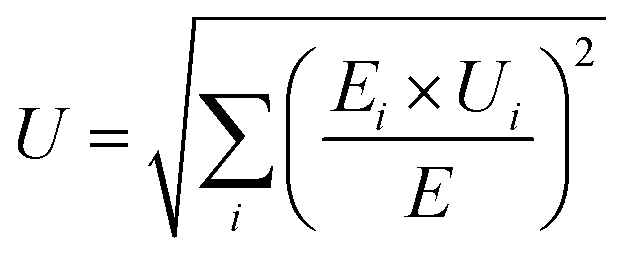
Finally, to derive the overall uncertainty on total Australian anthropogenic mercury emissions (U), we combined the individual sectoral uncertainties Ui, weighted by the contribution of the sectoral emissions Ei to total emissions E:
 | (2) |
Because both sectoral and total emissions vary annually, the overall uncertainty U also varies annually in our inventory.
2.2 Chemical transport modelling
To evaluate the implications of the updated emissions inventory for atmospheric mercury concentrations and deposition, we used the GEOS-Chem chemical transport model (CTM). The GEOS-Chem mercury simulation is described by Horowitz et al.,53 with updates to the atmospheric chemical mechanism described by Shah et al.54 Here we use the version described by Shah et al.,54 a modified version of GEOS-Chem v12.9.0.55 The GEOS-Chem mercury simulation dynamically couples a global 3-D atmosphere to ocean and terrestrial reservoirs, with ocean and land mercury concentrations provided as boundary conditions.53 The atmospheric simulation includes Hg0 and 24 forms of HgII, with chemical cycling including gas-phase oxidation reactions, gas-phase and aqueous-phase photolysis, and multiphase processes in aerosols and cloud droplets.54We simulated the full 2000–2019 period, preceded by a two-year spin-up (repeating spin-up year 1999), with our analysis primarily focused on the final three years of the simulation period (2017–2019). Our simulations were driven by assimilated meteorology from the NASA Modern-Era Retrospective Analysis for Research and Applications, version 2 (MERRA-2) reanalysis product.56 We perform global simulations at 2° × 2.5° resolution by downgrading the native MERRA-2 resolution (0.5° × 0.625°), as is standard for global GEOS-Chem mercury simulations.53,54 We used model timesteps of 10 minutes for transport and convection and 20 minutes for emission and chemistry. Mercury emissions are speciated into contributions from Hg0 and HgII, with online gas-particle partitioning of HgII following Amos et al.57 We used anthropogenic emissions as described below, along with biomass burning emissions from the Global Fire Emissions Database Version 4 (GFED4s)58 and natural emissions (including exchange with surface reservoirs) as described by Horowitz et al.53
We performed a suite of three model simulations: a base simulation and two sensitivity simulations. Only the anthropogenic emissions differed between the simulations. For the base simulation, we used the Streets et al.16 global anthropogenic emissions inventory outside of Australia, overwritten by our new inventory for Australia.
The first sensitivity simulation was designed to understand how changes in Australian anthropogenic emissions since 2000 have influenced present-day mercury concentrations in surface air and mercury deposition. While the 20-year simulation provides some indication, it is not sufficient to understand the anthropogenic influence because of contemporaneous changes in meteorology and other emissions (e.g., biomass burning, anthropogenic emissions from other countries). Instead, we repeated the final three years of our base simulation (2017–2019) using Australian anthropogenic emissions from the year 2000. All other parameters (meteorology, biomass burning emissions, initial conditions, etc.) remained unchanged from the base simulation, meaning any differences between the two simulations can be solely attributed to changes in Australian anthropogenic emissions since the year 2000.
The second sensitivity simulation was designed to understand how use of our new inventory changes simulated present-day mercury concentrations and deposition relative to the global inventory. To do so, we used the Streets et al.16 global anthropogenic emissions everywhere, including for Australia. For this simulation, we repeated the full 2000–2019 simulation period (starting from the same initial conditions as in the base simulation) to capture the impact of any differences in trends between the inventories. The final year of emissions data in the Streets et al.16 inventory is 2015, and so 2015 emissions are used for all subsequent years.
3 Results and discussion
3.1 Anthropogenic emissions and trends
The annually resolved, 20 year record of anthropogenic emissions summed over Australia is shown in Fig. 1, which presents the timeseries of total anthropogenic emissions (along with their uncertainties) shown as the sum of the absolute contributions from each sector, and Fig. 2, which shows the timeseries for each sector individually. Summed over sectors, total annual anthropogenic mercury emissions decreased by nearly 10 Mg over the past 20 years, from 18.6 Mg yr−1 in 2000 to 8.9 Mg yr−1 in 2019 (a decrease of 52%). Fig. 1 shows that this decrease is primarily due to the decreasing emissions in the gold production sector. As discussed previously by Fisher and Nelson,6 the dramatic decrease in gold production emissions can be attributed to a change at the Kalgoorlie gold processing facility from roasting (which vaporises the mercury and emits it to the atmosphere) to ultrafine grinding. The latter process grinds the ore into fine particles that then undergo a multi-step process that first adsorbs the particles onto activated carbon then strips the gold from the carbon. The mercury remains adsorbed onto the activated carbon rather than being emitted to the atmosphere.59 As a result of the upgrade, mercury emissions from gold production decreased by 8.2 Mg yr−1 from their peak in 2004, accounting for 75% of the total decrease in anthropogenic mercury emissions since then.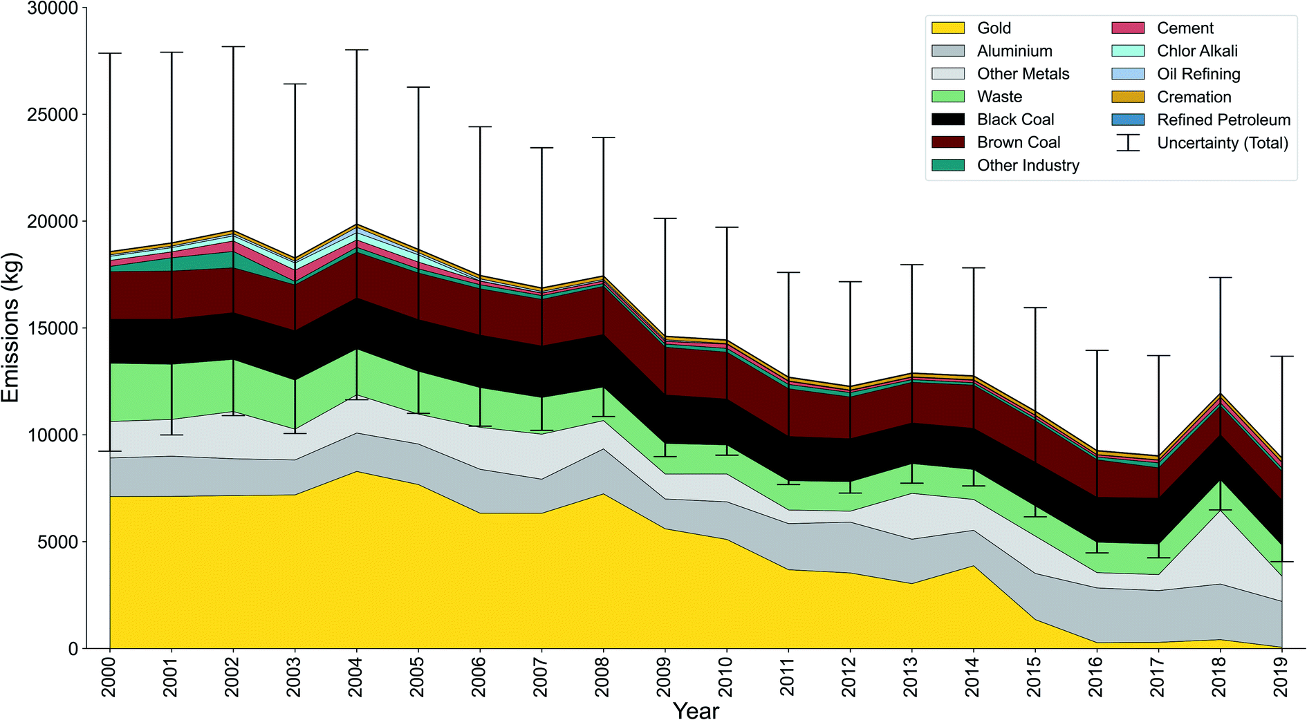 | ||
| Fig. 1 Annual Australian mercury emissions coloured by sector. Error bars represent the uncertainty on total mercury emissions, calculated as described in Section 2.1.4. | ||
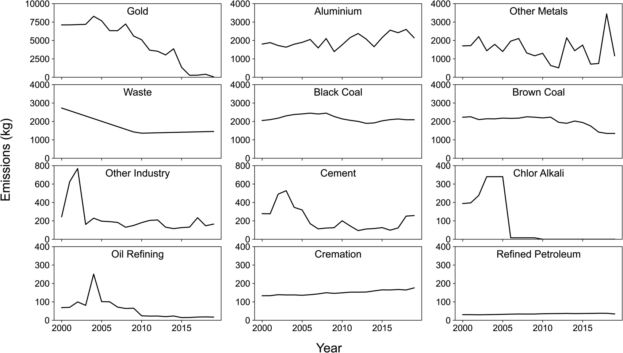 | ||
| Fig. 2 Annual anthropogenic mercury emissions by sector from 2000 to 2019. Note the different scales on each plot. | ||
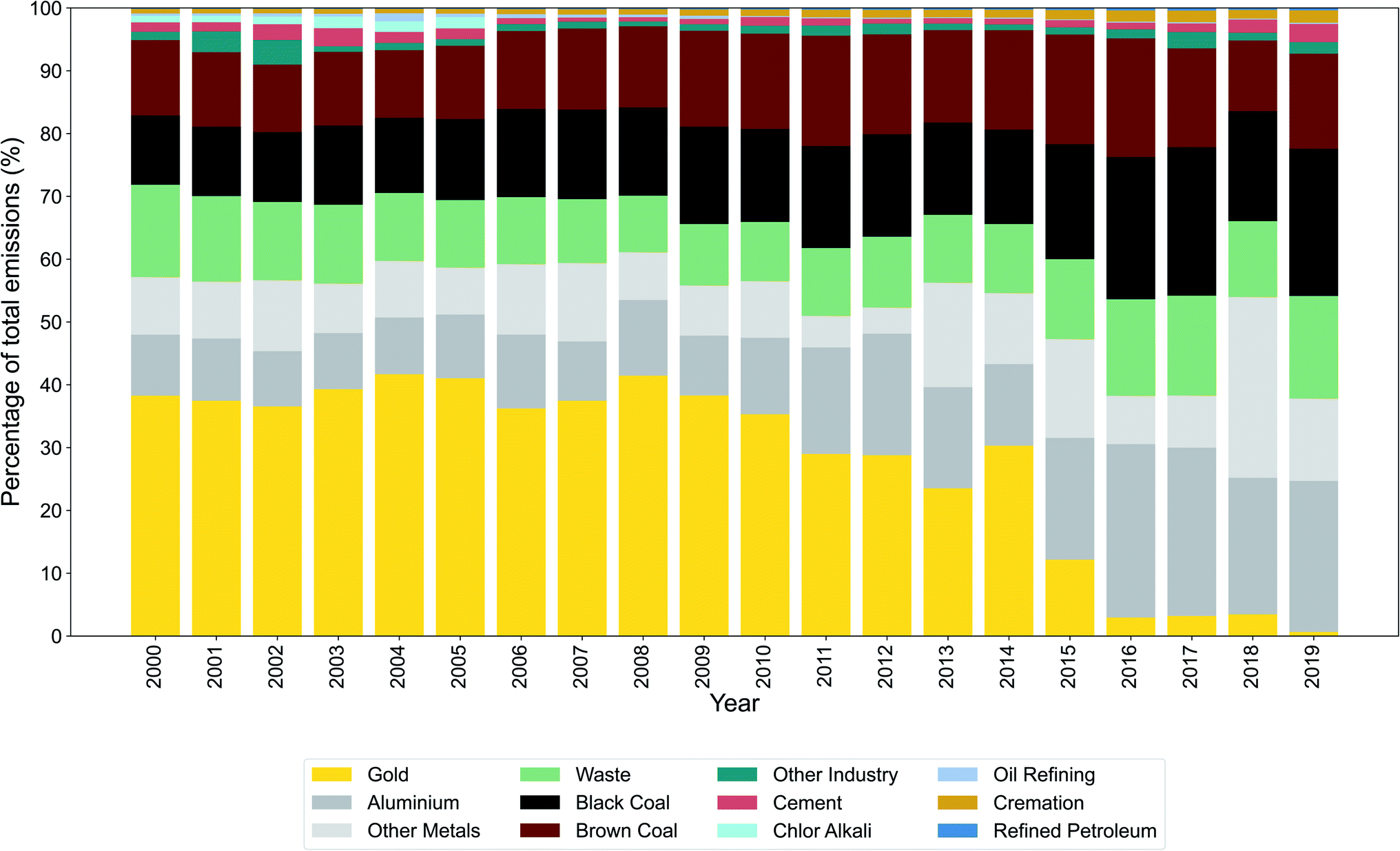
While the emissions decline was largest for the gold production sector, we find that mercury emissions from most other sectors also decreased over the two decades from 2000 to 2019. This can be seen qualitatively in Fig. 2. To quantify the change, we used the Mann–Kendall test (implemented in Python as pyMannKendall60) to test for the presence of a significant monotonic trend. For those sectors found to have a significant trend (with 95% confidence), we used the Theil-Sen estimator61,62 to calculate the magnitude of the trend. The results, shown in Table 4 in both absolute and relative units, show statistically significant trends in emissions from all sectors except black coal-fired power plants and production of “other” metals (excluding gold and aluminium). Decreasing trends were found for most sectors (gold production, commercial product waste, brown coal-fired power plants, cement production, oil refining, and chlor-alkali production), with increasing trends for only aluminium production, cremation, and refined petroleum products.
| Sector | Trend (kg yr−1) | Trend (% yr−1) |
|---|---|---|
| a Absolute trend (to the nearest kg except where less than 1 kg yr−1) calculated as the Theil-Sen slope where trends are found to be significant with 95% confidence using the Mann–Kendall test. “n.s.” indicates the trend was not significant. Relative trend calculated from the absolute trend based on the intercept (year 2000) value. Numbers to the right of each trend give the lower and upper 95% confidence estimates of the trend. b The annual waste emission estimates are interpolated linearly from the decadal estimates and therefore assume a continuous trend across each decade. Interannual variability in this source that is not captured in our inventory could render this trend insignificant. | ||
| Gold | −462−343−558 | −4.7−3.5−5.7 |
| Wasteb | −67−33−101 | −3.2−1.6−4.9 |
| Brown coal | −31−15−52 | −1.3−0.6−2.1 |
| Cement | −9−1−19 | −3.9−0.5−7.8 |
| Other industry | −6−2−11 | −2.4−0.6−4.5 |
| Oil refining | −5−2−7 | −5.2−2.3−7.9 |
| Chlor-alkali | −2−0−18 | −8.3−0.1−93 |
| Refined petroleum | +0.5+0.5+0.4 | +1.6+1.8+1.4 |
| Cremation | +2+2+2 | +1.6+1.9+1.4 |
| Aluminium | +38+57+16 | +2.3+3.5+1.0 |
| Black coal | n.s. | n.s. |
| Other metals | n.s. | n.s. |
| Total | −610 −502 −729 | −3.0 −2.5 −3.6 |
As shown in Table 4, trends in most sectors were small in absolute terms, with changes of <10 kg yr−1 (<200 kg over the 20 year study period). The exceptions (in addition to the gold production sector discussed above) were emissions from commercial product waste (−67 kg yr−1 or −1300 kg over 20 years), brown coal-fired power plants (−31 kg yr−1 or −600 kg over 20 years), and aluminium production (+38 kg yr−1 or +800 kg over 20 years). The decrease in emissions from commercial product waste can be explained by the lag between product consumption and disposal (Section 2.1.2), with peak mercury consumption in earlier decades14 influencing the quantity of mercury-containing waste and associated emission. Larger air emission factors in 2000 than in later decades driven by changes to disposal practices (e.g., increased recycling; Appendix 1) also play a role.
The decrease in emissions from brown coal-fired power plants can be attributed to the closure of a number of power stations, in particular the Hazelwood power station in Victoria's Latrobe Valley. Prior to its closure in 2017, Hazelwood alone emitted around 500 kg yr−1, accounting for 20–25% of emissions from the brown coal-fired power plant sector. The closure of Hazelwood power station was preceded by closure of several smaller brown coal-fired power stations between 2012 and 2016 (including Playford and Northern in South Australia and Morwell and Angelsea in Victoria), collectively accounting for mercury emissions of around 150 kg yr−1 before 2012. Combined, these closures drove a decrease in mercury emissions from brown coal over the past decade (Fig. 2).
The aluminium sector (including mining, refining and production of aluminium, alumina and bauxite ore) was the only sector with a notable emission increase from 2000 to 2019. The bulk of aluminium sector emissions come from six bauxite facilities: Worsley, Kwinana, Wagerup, Pinjarra (all in Western Australia), Queensland Alumina Limited (Queensland), and Gove (Northern Territory). The growth in aluminium sector emissions can be attributed to increasing emissions from the Western Australian refineries since 2009; meanwhile, emissions from Queensland Alumina Limited decreased over the study period, and the Gove refinery closed in 2014. The mercury emissions trend found here is consistent with Australian bauxite production and export trends and may be linked to growth in Chinese imports over this period.63 Despite a brief downturn in 2020, aluminium and bauxite production are projected to grow in coming years,63 potentially leading to further growth in aluminium sector mercury emissions.
The growth in emissions from the aluminium sector combined with declines in most other sectors has led to a redistribution of the relative importance of the different anthropogenic mercury sources. As shown in Fig. 3 and Table 5, Australia's controllable primary mercury emissions can now largely be attributed to two sectors: electricity from coal-fired power plants (39%) and production of aluminium and other non-gold metals (37%). Within the coal-fired power plant sector, we find that emissions from black and brown coal-fired power plants were roughly equivalent from 2000 to 2016. Following the 2017 closure of Hazelwood discussed above, black coal-fired power plants now account for roughly 60% of sectoral emissions (Table 5).
 | ||
| Fig. 3 Relative contribution of each sector to total Australian anthropogenic mercury emissions in each year. | ||
| Sector | 2019 emissions |
|---|---|
| a Nickel, iron, steel, zinc, magnetite, manganese, copper, lead, lithium, uranium, and mixed metals. | |
| Aluminium | 2150 |
| Black coal | 2090 |
| Waste | 1460 |
| Brown coal | 1350 |
| Other metalsa | 1170 |
| Cement | 257 |
| Cremation | 176 |
| Other industry | 165 |
| Gold | 58 |
| Refined petroleum | 34 |
| Oil refining | 17 |
| Chlor-alkali | 0 |
| Total | 8920 |
Within the metal production sector, roughly two thirds of emissions come from the aluminium sector discussed above (Table 5). Emissions from production of other metals (i.e., not gold or aluminium) are dominated by “mixed metals” (typically 60–80% of sectoral emissions), followed by nickel (15–25% of sectoral emissions). Mixed metals are reported as such in the NPI, preventing further delineation by metal type. On average, mixed metal production is responsible for mercury emissions of 1000 kg yr−1, but with large variability (range of 200–3300 kg yr−1). Inspection of the NPI database shows that a single facility, Mount Isa Mines, dominates both the magnitude and the variability of the mixed metal category, reporting annual emissions that range from 14 to 3100 kg yr−1 with a median annual value of 600 kg yr−1. We expect the extremely large variability is due to inconsistent reporting to the NPI database, rather than any true variability in emissions. In an examination of lead emissions, Cooper et al.64 previously found that Mount Isa Mines reported emissions to the NPI using up to seven different estimation methods within 14 years.64 While this inconsistency has only been explicitly identified for lead, the same inconsistent reporting may apply to mercury emissions. The large increase in 2018 in particular (Fig. 2) may be a reporting error. Mercury emissions from the mixed metal sector remain an important uncertainty in our inventory, especially in recent years where they account for more than 10% of total anthropogenic mercury emissions (Table 5).
As shown in Table 5, our best estimate of present-day Australian anthropogenic mercury emissions is 8.9 Mg yr−1, consistent with the 5–10 Mg yr−1 suggested by Fisher and Nelson.6 We also compare our new inventory to two recent independent estimates from global inventories: Streets et al.16 and the GMA2018.11 The Streets et al.16 inventory for Oceania is similar to the WHET inventory12 discussed in detail by Fisher and Nelson6 but with updates to fossil fuel combustion sources.6 As in Fisher and Nelson,6 we estimate Australian emissions from total Oceania emissions assuming Australia accounts for 81% of total Oceania emissions in each sector (excluding artisanal-scale gold mining, which takes place exclusively outside of Australia). For the GMA2018 inventory, the Technical Background Report11 provides Australian-level emission estimates, which we use directly. To ensure consistency in the comparison, we lump emissions from each inventory into the five overarching categories used by Fisher and Nelson6 and further split “other metals” into aluminium and non-aluminium metals. We compare emissions estimates for 2015, the only year of overlap between all three inventories.
Fig. 4 shows 2015 emissions from our inventory compared to those from the Streets and GMA2018 global inventories. Total emissions estimated with our inventory are roughly 50% higher than those from the GMA2018 and 50% lower than those from Streets. At the sector-level, the figure shows that the largest differences are in the waste, gold, and aluminium sectors. The Streets inventory overestimates emissions from commercial product waste because they assumed that Oceania's share of global consumption was the same in earlier decades as in 2010 (see Fisher and Nelson6 discussion for WHET, which used the same waste emissions). In reality, the Oceania share of consumption more than doubled from 1990 to 2010 (Appendix 1), so applying the 2010 value to historical consumption data significantly overestimates historical consumption and contemporary disposal and emissions. The Streets inventory also overestimates 2015 gold production emissions, with values that are representative of the Kalgoorlie facility before the transition from roasting to grinding. Mercury emissions from aluminium production are not considered in the Streets inventory.
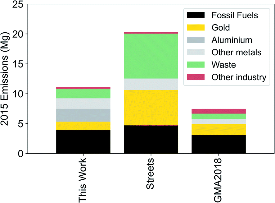 | ||
| Fig. 4 Total Australian anthropogenic mercury emissions (Mg) in 2015 from (left to right) this work, Streets et al.,16 and the GMA2018,11 separated into six consistent sectors. | ||
In contrast, emissions from the GMA2018 inventory are lower than in our new inventory for most sectors. The GMA2018 does not account for delays between consumption and disposal of commercial products, explaining the lower waste emissions. Differences in aluminium, gold, other metals, and other industry (mainly cement) can be attributed to methodological differences, with the GMA2018 estimates based on country-level activity data (e.g., total aluminium produced) versus the facility-level NPI emissions used here. For coal-fired power plants, we find the GMA2018 underestimates emissions by using a mercury capture rate of 46.5% for brown (sub-bituminous) coal combustion. This value originates from the 2005 NPI Emission Estimation Technique Manual recommendation for black coal-fired power plants with ESPs65 and is significantly higher than the 2% capture rate recommended for brown coal-fired power plants in the updated 2012 NPI Emission Estimation Technique Manual.19 For black coal combustion, the GMA2018 also uses higher mercury capture rates (46% for ESPs, 83% for FFs) than now recommended by the NPI (19% for both); however, the resulting underestimate is compensated by a higher assumed black coal mercury content in the GMA2018 (0.068 ppm) than used in our work (0.05 ppm; see Section 2.1.1). Based on these findings, we recommend an update to the assumptions used for Australian coal combustion emissions in the next iteration of the Global Mercury Assessment.
3.2 Implications for atmospheric mercury and mercury deposition
Fig. 5a shows the present-day (2017–2019) spatial distribution of gaseous elemental mercury (Hg0) and oxidised mercury (HgII) concentrations in surface air over Australasia, as modelled by GEOS-Chem using our base simulation driven by our new anthropogenic emissions inventory (Section 2.2). Also shown are mean observed Hg0 concentrations from Cape Grim66 (Tasmania) and Gunn Point67 (Northern Territory), the only Australian monitoring sites with multi-year records.6 The existing observations are not sufficient to quantitatively evaluate the simulation given (1) their limited spatial coverage and distance from Australian anthropogenic emission sources, (2) uncertainties and concerns about data quality at the Cape Grim site,6 and (3) the difference in spatial scale between the single-point measurements and the model grid. Nonetheless, they provide a rough indication of the concentrations in the region.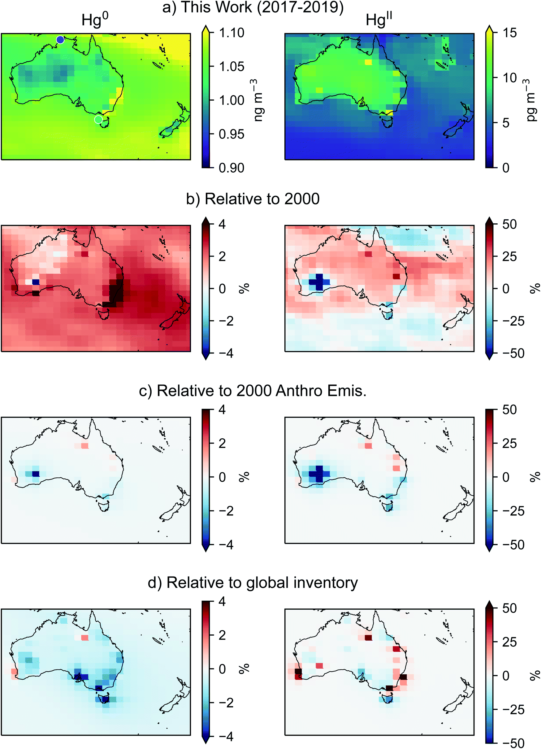 | ||
| Fig. 5 (a) Mean concentration of elemental mercury (Hg0, left) and oxidised mercury (HgII, right) in surface air as simulated by GEOS-Chem for 2017–2019 using the new Australian anthropogenic emissions inventory derived in this work (base simulation). For Hg0, overlay circles show published mean observed concentrations at Cape Grim66 and Gunn Point.67 (b–d) Relative difference in simulated Hg0 and HgII in surface air between the base simulation for 2017–2019 and: (b) the base simulation for the year 2000; (c) a sensitivity simulation for 2017–2019 using the year 2000 Australian anthropogenic emissions; (d) a sensitivity simulation for 2017–2019 using the Streets et al.16 global inventory for Australian anthropogenic emissions. All relative differences are calculated as (base-sensitivity)/sensitivity. For a larger regional perspective, see Fig. S2 in the ESI.† | ||
The figure shows that mean Australian Hg0 concentrations in the base simulation are roughly 1 ng m−3, consistent with observations68 and models11 of the Southern Hemisphere Hg0 background. Over coastal regions, the modelled values are generally consistent with the Australian observations from coastal sites (Gunn Point and Cape Grim) of 0.9–1.0 ng m−3 (ref. 66 and 67) (as shown overlay in Fig. 5a). Inland, simulated Hg0 concentrations are somewhat lower, but still higher than the 0.7 ng m−3 observed by MacSween et al.69 during a 1 year field campaign. Simulated mean HgII concentrations are more variable, ranging from near-zero over the ocean to 16 pg m−3 near emission hotspots, with average values over Australia closer to 10 pg m−3. Measurements of HgII in this region are even more scarce than for Hg0,6 with the longest available dataset (6 months using a Tekran 2537/1130) showing mean concentrations of 11 pg m−3 near Sydney70 that are roughly consistent with our simulations (noting large uncertainties in Tekran HgII measurements71).
To provide an indication of change over time, Fig. 5b compares the simulated surface air mercury concentrations for 2017–2019 to those for the year 2000 (i.e., the first year of our study period), both from the base simulation. Some features of the concentration differences are consistent with the anthropogenic emissions trends discussed in Section 3.1, such as the large decrease in both Hg0 and HgII concentrations in southwest Australia at the location of the Kalgoorlie gold processing facility (see Fig. S1 in the ESI† for emission maps). However, trends and interannual variability in other parameters confound interpretation of the differences. For example, the extreme fires in southeast Australia in late 2019 (ref. 72 and 73) led to enhancements in simulated Hg0 that more than compensated for the decreased emissions from waste and power plants in this region.
We removed the influence of other parameters by instead comparing the base run to a sensitivity simulation that replaced present-day Australian anthropogenic emissions with year 2000 Australian anthropogenic emissions (both from our new inventory). The simulations are otherwise identical (see Section 2.2), and so all differences can be attributed to temporal changes in Australian anthropogenic emissions between 2000 and present-day (2017–2019). Fig. 5c shows the relative difference between the two simulations, both averaged over 2017–2019. Consistent with the emission trends described in Section 3.1, concentrations of both Hg0 and HgII generally decrease over time, with the largest change found in the vicinity of the Kalgoorlie gold processing facility in southwest Australia. Moderate decreases are also seen across southeast Australia, reflecting the emissions reductions from brown coal-fired power plants and commercial product waste. Small increases in both Hg0 and HgII are associated with metal production from alumina refineries in Perth and other metal facilities in Queensland, including Mount Isa Mines (northwest Queensland). We note that our comparison period includes the year 2018, when we suspect NPI reporting errors led to unexpectedly large mixed metal emissions from Mount Isa Mines (see Section 3.1) and therefore likely overestimates the increase at this site. Nonetheless, even when 2018 is excluded from the comparison, we still find small increases in Hg0 and HgII concentrations at Mount Isa (not shown).
The differences in surface air concentrations are reflected in total Hg0 and HgII deposition, shown in Fig. 6. Comparing the base run in 2017–2019 to the same run in 2000 (Fig. 6b) and to the sensitivity run using year 2000 Australian anthropogenic emissions (Fig. 6c) shows that the impact of changes in Australian anthropogenic emissions is generally dwarfed by the impact of changes in other variables except near Kalgoorlie. In fact, for HgIIFig. 6b shows that in some places (e.g., central Australia, Southern Ocean) the deposition differences are opposite in sign to the concentration differences, presumably due to contemporaneous changes in precipitation over this period. We tested the output from the base run for trends in Australian Hg0, HgII, and total mercury deposition over the 2000–2019 simulation period. Despite the decreasing trend in anthropogenic emissions (Section 3.1), we did not detect a statistically significant trend in deposition, again pointing to the influence of interannual variability in precipitation, biomass burning emissions, and potentially other variables. In addition, HgII wet deposition strongly depends on oxidation in the free troposphere,74 which would be less impacted by Australian surface emissions. Nonetheless, we find using the sensitivity simulation that 4 Mg yr−1 (∼3–4%) less HgII is deposited to the Australian continent with present-day anthropogenic emissions than year 2000 emissions. Differences in total Hg0 deposition were negligible (<1%); however, our simulations did not account for changes to secondary re-emission from soil and ocean sources, which would also be expected to decrease in response to the emission changes.
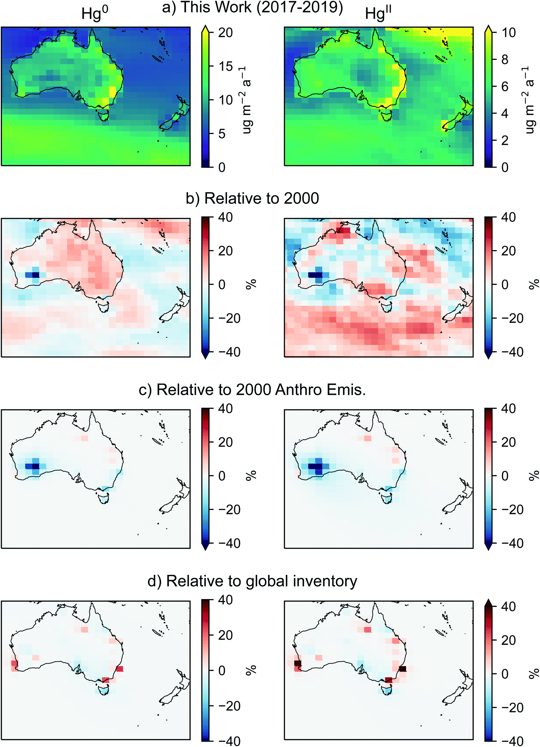 | ||
| Fig. 6 Same as Fig. 5 but for deposition of Hg0 (dry deposition and ocean uptake) and HgII (wet and dry deposition). For a larger regional perspective, see Fig. S3 in the ESI.† | ||
We used a second sensitivity simulation to understand the impact of modelling Australian anthropogenic emissions using our new inventory rather than a global inventory. Fig. 5d compares the surface air mercury concentrations from the base run using our new inventory to a sensitivity simulation that instead uses the Streets et al.16 global anthropogenic emissions inventory for Australia (see Section 2.2). Consistent with the inventory comparisons shown in Fig. 4, driving the model with our new inventory results in lower Hg0 concentrations across most of Australia. The only exceptions are locations where most emissions derive from metal production (alumina refineries in the southwest, Mount Isa Mines in the north), which we found to be underestimated in the global inventory (see Section 3.1). Despite the large differences in total emissions between the two inventories, differences in Hg0 concentration are only of order 5% over Australian emission hotspots and negligible elsewhere. These results highlight the relatively minor contribution of Australian anthropogenic emissions to Hg0 surface air concentrations, both locally and downwind, consistent with previous model findings that most Hg0 in this region can be attributed to natural sources.11,75,76
For HgII, differences are more heterogenous and larger in magnitude. The base run (using our inventory) displays lower HgII concentrations in populous parts of the country around Adelaide, Melbourne, and Tasmania, likely due to the substantially lower waste emissions (Fig. 4), which scale spatially with population density. However, in several emission hotspots, HgII is higher in the base run, in some cases by more than 40% (Fig. 5d). Except in the few locations where Hg0 was also higher in the base run, the increase in HgII reflects different speciation between the two inventories. Comparing speciation fractions from our inventory to those from Streets et al.16 (Table S2†) shows similar values for most sectors except production of cement (76% HgII in this work versus 49% HgII in Streets et al.16) and most non-ferrous metals (50–68% HgII in this work versus 20–36% HgII in Streets et al.16 for gold, copper, lead, and zinc). The differences in Fig. 5d indicate that in many cases, the choice of speciation factors has a more significant impact on HgII concentrations than the overall quantity of emissions.
Similarly, Fig. 6d shows that simulated HgII deposition is generally higher when using our new inventory, at least near major emission hotspots. Summed over Australia, we find mean present-day (2017–2019) annual HgII deposition of 105.2 Mg yr−1 using our inventory versus 105.0 Mg yr−1 using the global inventory—a negligible difference that is much smaller than the uncertainties. Examining the entire 2000–2019 period shows larger differences in the first years of the simulation, with mean annual HgII deposition over Australia that is 5 Mg yr−1 (∼5%) larger with our inventory than the global inventory during 2000–2002. Although the difference between inventories decreases with time, we find that summed over the entire 2000–2019 period, using our inventory results in an additional 61 Mg of HgII deposition to the Australian landscape. Changes to Hg0 dry deposition are smaller and opposite in sign (as expected from the change in speciation). With both species combined, we find an increase in total Australian mercury deposition of 49 Mg when using our inventory. This estimate does not take into account re-volatilisation and subsequent re-deposition of this additional mercury and therefore represents a lower limit of the overall difference.
4 Conclusion
We have developed an updated, Australia-specific spatially resolved anthropogenic mercury emissions inventory with annual resolution from 2000 to 2019 using data from a variety of Australian sources. The inventory is open access and can be downloaded from https://doi.org/10.5281/zenodo.6383431. Our new inventory showed that Australian anthropogenic mercury emissions have undergone significant change over the past 20 years, with a decrease in total annual anthropogenic emissions of 10.3 Mg. Most of this decrease was due to the elimination of mercury emissions from a single gold production facility in Kalgoorlie, Western Australia. There have also been significant decreases in emissions from brown coal-fired power plants due to power plant closures and from waste due to the reduced mercury use in commercial products and changing disposal practices. Only the aluminium sector has experienced notable growth in emissions, mostly likely linked to export demand. Mercury emissions from production of aluminium and other metals are now on par with emissions from coal-fired power plants, and projections of future growth in aluminium and bauxite production imply this source may become increasingly prominent. These shifts in the sectoral distribution of emission sources have implications for developing appropriate regulatory actions to reduce Australian atmospheric mercury emissions.Using the GEOS-Chem chemical transport model, we evaluated the implications for atmospheric mercury concentrations and deposition in the Australasian region. We found that the decrease in Australian anthropogenic mercury over the past two decades resulted in significant decreases in Australian HgII concentration and deposition, with a maximum decrease around the Kalgoorlie gold production facility in Western Australia and smaller decreases along the east coast of Australia. When only changes in Australian anthropogenic emissions were considered, we found a decrease in Australian HgII deposition from 2000 to present-day of 4 Mg yr−1. However, contemporaneous changes in precipitation and other drivers (e.g., biomass burning emissions) make for a more complex picture, with increased deposition in some parts of the region and no significant trend over time.
We found that Australian emissions are not accurately represented in current global anthropogenic emission inventories, with differences of roughly a factor of two in total Australian emissions from our inventory relative to the GMA2018 (ref. 11) and Streets et al.16 global inventories. Sectoral distributions also differed between the inventories, with implications for the spatial distributions of emissions (and therefore deposition). The GEOS-Chem model results showed a bigger impact on mercury concentration and deposition from using an inaccurate global emission inventory than from the temporal trends in emissions. Model studies of source attribution and source–receptor relationships that underlie scientific and policy analysis rely on global emission inventories for consistency (e.g.,11,75,77). Our work highlights the need for assumptions about Australian emissions to be revisited in global inventories.
Our model results suggest present-day total Australian mercury deposition is 228 Mg yr−1 (123 Mg yr−1 Hg0, 105 Mg yr−1 HgII), much larger than the <10 Mg yr−1 of mercury now emitted from Australian anthropogenic sources. The remainder comes from natural emissions (including biomass burning, soil re-emission, and marine emissions) and transported anthropogenic emissions from other countries. The contribution from Australian soils remains a particularly large uncertainty: while some model studies suggest a very large soil source,8 recent observations show a balance between soil emission and uptake resulting in a near-zero net flux.69,69,78 Development of improved, observationally-constrained Australian soil flux parameterisations remains a key research priority for Australian mercury science. Meanwhile, the contribution from transported anthropogenic emissions indicates a significant benefit to Australia from the Minamata Convention: with the relatively small impact of local anthropogenic emissions shown here, Australia stands to gain from the reductions in global anthropogenic emissions expected to arise in response to the Convention.
5 Appendix 1
This appendix describes the methodology used to estimate mercury emissions from disposal of mercury-containing products. As described in the main text, we calculated these emissions for four categories defined by Horowitz et al.:14 lamps (all types of mercury-containing lightbulbs, including fluorescent, high intensity discharge, etc.), batteries (button cells and cylinders using mercury as cathode or to prevent corrosion), medical devices (thermometers and sphygmomanometers), and wiring and measuring devices (switches and relays, thermostats, barometers, manometers). We calculated emissions at decadal scale for 2000, 2010, and 2020 as described here (then interpolated to annual scale as described in the main text). For each product and year, we first calculated Oceania consumption, then Australian consumption, then Australian disposal, and finally Australian emission.Oceania consumption
For lamps, batteries, and medical devices, we did not consider delayed disposal (on the decadal scale), so only data from 2000–2020 were needed.For lamps and batteries, consumption data came directly from Wilson et al.43 for 2000 and the GMA2013 Technical Background Report for 2010.7 For 2020, we extrapolated the 5-yearly 2005–2015 consumption data from Wilson et al.,43 the GMA2013 Technical Background Report,7 and the UN Environment for 2015.44
For medical devices, Horowitz et al.14 calculated the “developed world” (Oceania, North America, Western Europe) consumption for 1990, 2000 and 2010, and Zhang et al.12 then determined the Oceania fraction of the developed world consumption for each of those years. Here, we calculated Oceania consumption for 1990, 2000, and 2010 directly from those values. For 2020, we extrapolated the developed world consumption to 2020 and applied the 2010 Oceania consumption fraction (we found this method produced a monotonic decreasing trend, whereas extrapolating the noisier consumption fraction led to an unexpected increase in 2020, although the differences were <50 kg).
For wiring and measuring devices, we calculated decadal scale consumption starting from 1950, as the earlier data are necessary for the eventual calculation of delayed disposal and emission. We started from the global and developed world consumption data from Horowitz et al.,14 shown in Table 6.
To calculate the Oceania consumption, we needed to know the fraction of total world (1950–1960) and developed world (1970–2010) consumption that can be attributed to Oceania. Wilson et al.43 reported regional and global consumption values from 1990–2005, with similar data for 2010 reported in the GMA2013 Technical Background Report.7 We used these data to calculate the Oceania fraction of developed world consumption for 1990, 2000, and 2010. In the absence of historical regional information, we assumed the 1990 consumption patterns are representative of earlier decades. We therefore used the 1990 value for the Oceania fraction of developed world consumption in 1970–1980. We also used the Wilson et al.43 data to calculate the Oceania fraction of total world consumption in 1990 for 1950–1960. Table 7 shows the resulting decadal Oceania consumption fractions.
| 1950 | 1960 | 1970 | 1980 | 1990 | 2000 | 2010 | |
|---|---|---|---|---|---|---|---|
| a Defined as Oceania, North America, and western Europe. Based on data from Wilson et al.43 for 1970–2000, with 1990 value used for earlier decades, and the GMA2013 Technical Background Report7 for 2010. b Only used for 1950–1960, when developed world data are not available. Based on 1990 data from Wilson et al.43 | |||||||
| Developed worlda | — | — | 0.028 | 0.028 | 0.028 | 0.050 | 0.064 |
| Total worldb | 0.013 | 0.013 | — | — | — | — | — |
Finally, we applied the Oceania consumption fractions in Table 7 to the consumption totals in Table 6 to derive Oceania consumption of mercury in wiring and measuring devices. These values, along with the Oceania consumption of mercury in other products described above, are shown in Table 8.
| 1950 | 1960 | 1970 | 1980 | 1990 | 2000 | 2010 | 2020 | |
|---|---|---|---|---|---|---|---|---|
| a For lamps, batteries, and medical devices, no delayed disposal is assumed so only 2000–2020 values are needed. b For wiring and measuring devices, disposal (and associated emission) is assumed to occur at least 10 years after consumption, so 2020 values are not needed. | ||||||||
| Lampsa | — | — | — | — | — | 2 | 2 | 3 |
| Batteriesa | — | — | — | — | — | 4 | 2 | 0 |
| Medical devicesa | — | — | — | — | — | 4 | 0.1 | 0.1 |
| Wiring & measuring devicesb | 6 | 12 | 17 | 11 | 11 | 7 | 6 | — |
Australian consumption
For all product categories, we determined the fraction of Oceania consumption that can be attributed to Australia using Gross Domestic Product at Purchasing Power Parity (GDP-PPP) from the World Bank,45 following AMAP/UNEP.52 GDP-PPP data are only available from 1990, so we again assumed the 1990 distribution is representative of earlier decades.We calculated total Oceania GDP-PPP by summing GDP-PPP for all countries included in the Wilson et al.43 definition of Oceania (defined in ref. 7). This definition was used to calculate the Australian fraction of Oceania consumption for lamps, batteries, and wiring and measuring devices, as the Oceania values for these categories all originate from Wilson et al.43 data. For medical devices, the Oceania consumption comes directly from Horowitz et al.,14 who used a slightly different definition of Oceania that includes Papua New Guinea (as defined in ref. 15). For this category, we therefore re-calculated the Australian fraction of Oceania inclusive of Papua New Guinea.
Australian consumption fractions are shown in Table 9. We applied these to the Oceania consumption data in Table 8 to derive the decadal Australian consumption estimates shown in Table 10.
| 1950 | 1960 | 1970 | 1980 | 1990 | 2000 | 2010 | 2020 | |
|---|---|---|---|---|---|---|---|---|
| a For lamps, batteries, and medical devices, no delayed disposal is assumed so only 2000–2020 values are needed. b For wiring and measuring devices, disposal (and associated emission) is assumed to occur at least 10 years after consumption, so 2020 values are not needed. | ||||||||
| Lampsa | — | — | — | — | — | 1.7 | 1.7 | 2.5 |
| Batteriesa | — | — | — | — | — | 3.3 | 1.7 | 0.0 |
| Medical devicesa | — | — | — | — | — | 3.2 | 0.1 | 0.1 |
| Wiring & measuring devicesb | 4.9 | 9.8 | 14 | 9.0 | 9.1 | 5.5 | 4.9 | — |
Australian disposal
We next used the estimated Australian consumption values from Table 10 to estimate disposal. As in Horowitz et al.,14 we assumed delayed (>10 year) disposal only for the wiring and measuring devices; for all other categories, at the decadal scale used here, disposal was assumed to equal consumption.For wiring and measuring devices, we applied the same delays as in Horowitz et al.14 10% disposal occurs 10 years after consumption, 40% disposal after 30 years, and 50% disposal after 50 years. This means, for example, that disposal in the year 2020 is the sum of 10% of the 2010 consumption (10 year delay between consumption and disposal), 40% of the 1990 consumption (30 year delay), and 50% of the 1970 consumption.
Estimates of Australian mercury product disposal derived using these assumptions (applied to the data in Table 10) are shown in Table 11. As emissions occur at the disposal stage, only 2000–2020 disposal values are relevant to this work.
Mercury air emission factors
Mercury air emission factors represent the fraction of disposed mercury that is emitted to the atmosphere during the disposal process. We calculated mercury air emission factors using the air distribution factors from Horowitz et al.14 For each product type, Horowitz et al.14 determined the fractional distribution of different disposal methods (e.g., landfill versus incineration versus recycling) for each decade from 1990 to 2010, as well as the air emission factor associated with each disposal method. These terms were combined to derive an overall air distribution factor (i.e., air emission factor) for each disposal method and product type, and then summed over different disposal methods to give the total air distribution factor (for each decade).We used the Horowitz et al.14 values directly for 2000 and 2010. For 2020, we extrapolated the Horowitz et al.14 air distribution factors for each disposal method and product to 2020 and then summed over disposal methods to give the total air emission factor for each product for 2020 (rather than extrapolating the summed value). The resultant air emission factors are shown in Table 12.
Mercury emissions from Australian product disposal
Finally, we applied the air emission factors from Table 12 to the Australian mercury disposal estimates from Table 11 to calculate total Australian emissions from disposal of mercury-containing products, shown in Table 13. These were then interpolated to annual scale and distributed spatially as described in the main text.Conflicts of interest
There are no conflicts to declare.Acknowledgements
This work was undertaken with the assistance of resources provided at the National Computational Infrastructure (NCI) National Facility systems at the Australian National University through the National Computational Merit Allocation Scheme (project m19) supported by the Australian Government. This project was supported by the University of Wollongong Global Challenges Program. We gratefully acknowledge David Streets for his contribution to the original commercial products waste emissions estimates that we adapted in this work.References
- C. A. Eagles-Smith, E. K. Silbergeld, N. Basu, P. Bustamante, F. Diaz-Barriga, W. A. Hopkins, K. A. Kidd and J. F. Nyland, Modulators of mercury risk to wildlife and humans in the context of rapid global change, Ambio, 2018, 47, 170–197 CrossRef.
- C. T. Driscoll, R. P. Mason, H. M. Chan, D. J. Jacob and N. Pirrone, Mercury as a Global Pollutant: Sources, Pathways, and Effects, Environ. Sci. Technol., 2013, 47, 4967–4983 CrossRef CAS.
- D. Obrist, J. L. Kirk, L. Zhang, E. M. Sunderland, M. Jiskra and N. E. Selin, A review of global environmental mercury processes in response to human and natural perturbations: changes of emissions, climate, and land use, Ambio, 2018, 47, 116–140 CrossRef.
- H. Hsu-Kim, C. S. Eckley, D. Achá, X. Feng, C. C. Gilmour, S. Jonsson and C. P. J. Mitchell, Challenges and opportunities for managing aquatic mercury pollution in altered landscapes, Ambio, 2018, 47, 141–169 CrossRef PubMed.
- H. Selin, S. E. Keane, S. Wang, N. E. Selin, K. Davis and D. Bally, Linking science and policy to support the implementation of the Minamata Convention on Mercury, Ambio, 2018, 47, 198–215 CrossRef.
- J. A. Fisher and P. F. Nelson, Atmospheric mercury in Australia, Elementa, 2020, 8, 070 Search PubMed.
- AMAP/UNEP, Technical Background Report for the Global Mercury Assessment 2013, 2013, pp. 1–271 Search PubMed.
- P. F. Nelson, A. L. Morrison, H. J. Malfroy, M. Cope, S. Lee, M. L. Hibberd, C. P. M. Meyer and J. McGregor, Atmospheric mercury emissions in Australia from anthropogenic, natural and recycled sources, Atmos. Environ., 2012, 62, 291–302 CrossRef CAS.
- P. F. Nelson, Atmospheric emissions of mercury from Australian point sources, Atmos. Environ., 2007, 41, 1717–1724 CrossRef CAS.
- P. J. Burke, R. Best and F. Jotzo, Closures of coal-fired power stations in Australia: local unemployment effects, Aust. J. Agric. Resour. Econ., 2019, 63, 142–165 CrossRef.
- AMAP/UNEP, Technical Background Report to the Global Mercury Assessment 2018, 2019, pp. 1–430 Search PubMed.
- Y. Zhang, D. J. Jacob, H. M. Horowitz, L. Chen, H. M. Amos, D. P. Krabbenhoft, F. Slemr, V. L. St Louis and E. M. Sunderland, Observed decrease in atmospheric mercury explained by global decline in anthropogenic emissions, Proc. Natl. Acad. Sci. U. S. A., 2016, 113, 526–531 CrossRef CAS PubMed.
- M. Muntean, G. Janssens-Maenhout, S. Song, A. Giang, N. E. Selin, H. Zhong, Y. Zhao, J. G. J. Olivier, D. Guizzardi, M. Crippa, E. Schaaf and F. Dentener, Evaluating EDGARv4.tox2 speciated mercury emissions ex-post scenarios and their impacts on modelled global and regional wet deposition patterns, Atmos. Environ., 2018, 184, 56–68 CrossRef CAS.
- H. M. Horowitz, D. J. Jacob, H. M. Amos, D. G. Streets and E. M. Sunderland, Historical mercury releases from commercial products: global environmental implications, Environ. Sci. Technol., 2014, 48, 10242–10250 CrossRef CAS PubMed.
- D. G. Streets, H. M. Horowitz, D. J. Jacob, Z. Lu, L. Levin, A. F. H. ter Schure and E. M. Sunderland, Total Mercury Released to the Environment by Human Activities, Environ. Sci. Technol., 2017, 51, 5969–5977 CrossRef CAS PubMed.
- D. G. Streets, H. M. Horowitz, Z. Lu, L. Levin, C. P. Thackray and E. M. Sunderland, Global and regional trends in mercury emissions and concentrations, 2010–2015, Atmos. Environ., 2019, 201, 417–427 CrossRef CAS.
- National Pollutant Inventory, https://www.npi.gov.au/npidata/action/load/advance-search, accessed 5 December 2021 Search PubMed.
- Kalgoorlie Consolidated Gold Mines Pty Ltd, KCGM Gidji Roaster and Fimiston Carbon Kiln Stack Testing and Modelling Summary, 2005 Search PubMed.
- Department of Sustainability, Environment, Water, Population and Communities, National Pollutant Inventory emission estimation technique manual for fossil fuel electric power generation version 3.0, Environment Australia, Canberra, A.C.T., 2012 Search PubMed.
- Australian Energy Update 2020, https://www.energy.gov.au/publications/australian-energy-update-2020, accessed 26 June 2021 Search PubMed.
- D. J. Brockway and R. S. Higgins, in The science of Victorian brown coal, Elsevier, 1991, pp. 247–278 Search PubMed.
- R. Schofield, S. Utembe, C. Gionfriddo, M. Tate, D. Krabbenhoft, S. Adeloju, M. Keywood, R. Dargaville and M. Sandiford, Atmospheric mercury in the Latrobe Valley, Australia: Case study June 2013, Elementa, 2021, 9, 00072 Search PubMed.
- Electricity sector emissions and generation data, http://www.cleanenergyregulator.gov.au/NGER/National%20greenhouse%20and%20energy%20reporting%20data/electricity-sector-emissions-and-generation-data, accessed 31 May 2021 Search PubMed.
- Department of Sustainability, Environment, Water, Population and Communities, National Pollutant Inventory Emission Estimation Technique Manual for Crematoria v1.0, 2011 Search PubMed.
- L. Liang, M. Horvat and P. Danilchik, A novel analytical method for determination of picogram levels of total mercury in gasoline and other petroleum based products, Sci. Total Environ., 1996, 187, 57–64 CrossRef CAS.
- S. M. Wilhelm, Estimate of Mercury Emissions to the Atmosphere from Petroleum, Environ. Sci. Technol., 2001, 35, 4704–4710 CrossRef CAS PubMed.
- M. Garg, J. D. Silver, R. Schofield and R. G. Ryan, Hourly emission inventories for air toxic emissions for eastern Australian electricity generators derived from energy distribution data, Int. J. Environ. Sci. Technol., 2022, 19, 2973–2992 CrossRef CAS.
- L. S. Dale, Review of trace elements in coal, Australian Coal Association Research Program, 2003 Search PubMed.
- K. Riley, L. Dale, G. Devir, A. Williams and D. Holcombe, Background information for web site on trace elements in coal, Australian Coal Association Research Program, 2005 Search PubMed.
- Center for International Earth Science Information Network – CIESIN – Columbia University, Gridded Population of the World, Version 4 (GPWv4): Population Density, Revision 11, NASA Socioeconomic Data and Applications Center (SEDAC), Palisades, NY, 2018 Search PubMed.
- Australian Bureau of Statistics, Deaths, Year of registration, Summary data, Sex, States, Territories and Australia, https://explore.data.abs.gov.au/vis?fs[0]=ABS%20Topics%2C0%7CPEOPLE%23PEOPLE%23&fs[1]=ABS%20Topics%2C2%7CPEOPLE%23PEOPLE%23%7CPopulation%23POPULATION%23%7CDeaths%23DEATHS%23&pg=0&fc=ABS%20Topics&df[ds]=ABS_ABS_TOPICS&df[id]=DEATHS_SUMMARY&df[ag]=ABS&df[vs]=1.0.0&pd=2000%2C&dq=1%2B2%2B3%2B4%2B5%2B6%2B7%2B8%2B9%<?pdb_no 2B10?>2B10<?pdb END?>%<?pdb_no 2B11?>2B11<?pdb END?>.3.AUS.A&ly[cl]=TIME_PERIOD&ly[rw]=MEASURE, accessed 12 January 2022 Search PubMed.
- J. Barkla, Audit report – Crematoria industry sector (2016), 2016 Search PubMed.
- Australian Bureau of Agricultural and Resource Economics and Sciences, Mineral Energy Commodities Petroleum, https://www.awe.gov.au/sites/default/files/sitecollectiondocuments/abares/acs/2008/mineral-energy-commodities-petroleum.xls, accessed 20 April 2021 Search PubMed.
- Australian Bureau of Agricultural and Resource Economics and Sciences, Mineral Energy Commodities Petroleum, https://www.awe.gov.au/sites/default/files/sitecollectiondocuments/abares/acs/2010/mineral-energy-commodities-petroleum.xls, accessed 20 April 2021 Search PubMed.
- Australian Petroleum Statistics 2021, https://www.energy.gov.au/publications/australian-petroleum-statistics-2021, accessed 22 June 2021 Search PubMed.
- G. Lara-Rodriguez, O. Begovich and J. L. Naredo, Analysis of the Influence of LPG Density on the Performance of a Centrifugal Pump-Impeller Through CFD Simulations, Paper presented at the SPE Latin American and Caribbean Petroleum Engineering Conference, Quito, Ecuador, November 2015, SPE-177268-MS, OnePetro, 2015, DOI:10.2118/177268-MS.
- S. Sarıkoç, in Diesel and Gasoline Engines, ed. R. Viskup, 2020 Search PubMed.
- H. J. Curl and K. O'Donnell, Chemical and physical properties of refined petroleum products, Technical Memo, United States, 1977 Search PubMed.
- G. Hemighaus, T. Boval, J. Bacha, F. Barnes, M. Franklin, L. Gibbs, N. Hogue, J. Jones, D. Lesnini, J. Lind and J. Morris, Aviation Fuels Technical Review, Chevron Products Company, 2007 Search PubMed.
- S. M. Wilhelm and N. Bloom, Mercury in petroleum, Fuel Process. Technol., 2000, 63, 1–27 CrossRef CAS.
- J. H. Won, J. Y. Park and T. G. Lee, Mercury emissions from automobiles using gasoline, diesel, and LPG, Atmos. Environ., 2007, 41, 7547–7552 CrossRef CAS.
- Working Group on Mercury, Ambient air pollution by mercury (Hg): Position paper, European Communities, Luxembourg, 2002 Search PubMed.
- S. Wilson, J. Munthe, K. Sundseth, K. Kindbom, P. Maxson, J. M. Pacyna and F. Steenhuisen, Updating historical global inventories of anthropogenic mercury emissions to air, 2010 Search PubMed.
- UN Environment, Global mercury supply, trade and demand, United Nations Envrionment Programme, Chemicals and Health Branch, Geneva, Switzerland, 2017 Search PubMed.
- The World Bank, GDP, PPP (current international $), https://data.worldbank.org/indicator/NY.GDP.MKTP.PP.CD, accessed 15 November 2021 Search PubMed.
- S. M. Jasinkski, The Materials Flow of Mercury in the United States, United States Department of the Interior, 1994 Search PubMed.
- A. Cain, S. Disch, C. Twaroski, J. Reindl and C. R. Case, Substance Flow Analysis of Mercury Intentionally Used in Products in the United States, J. Ind. Ecol., 2007, 11, 61–75 CrossRef CAS.
- Russian Federal Service for Environmental, Technological and Danish Environmental Protection Agency, Assessment of Mercury Releases from the Russian Federation, Arctic Council, 2005 Search PubMed.
- P. Floyd, P. Zarogiannis, M. Crane, S. Tarkoswki and V. Bencko, Risks to health and the environment related to the use of mercury products, Risk & Policy Analysts Limited, 2002 Search PubMed.
- L. Zhang, S. Wang, Q. Wu, F. Wang, C.-J. Lin, L. Zhang, M. Hui, M. Yang, H. Su and J. Hao, Mercury transformation and speciation in flue gases from anthropogenic emission sources: a critical review, Atmos. Chem. Phys., 2016, 16, 2417–2433 CrossRef CAS.
- F. Wang, S. Wang, L. Zhang, H. Yang, Q. Wu and J. Hao, Mercury enrichment and its effects on atmospheric emissions in cement plants of China, Atmos. Environ., 2014, 92, 421–428 CrossRef CAS.
- AMAP/UNEP, Technical Background Report to the Global Atmospheric Mercury Assessment 2008, 2008, p. 159 Search PubMed.
- H. M. Horowitz, D. J. Jacob, Y. Zhang, T. S. Dibble, F. Slemr, H. M. Amos, J. A. Schmidt, E. S. Corbitt, E. A. Marais and E. M. Sunderland, A new mechanism for atmospheric mercury redox chemistry: implications for the global mercury budget, Atmos. Chem. Phys., 2017, 17, 6353–6371 CrossRef CAS.
- V. Shah, D. J. Jacob, C. P. Thackray, X. Wang, E. M. Sunderland, T. S. Dibble, A. Saiz-Lopez, I. Černušák, V. Kellö, P. J. Castro, R. Wu and C. Wang, Improved Mechanistic Model of the Atmospheric Redox Chemistry of Mercury, Environ. Sci. Technol., 2021, 55, 14445–14456 CrossRef CAS PubMed.
- B. Yantosca, M. Sulprizio, L. Lundgren, D. Kelvinhb, S. D. Eastham, R. Pound, T. Sherwen, H. Lin, J. Fisher, W. Downs, C. Thackray, C. michael-s-long, G. Luo, J. Zhuang, L. SpaceMouse, L. Murray, xin-chen-github noelleselin, gianga emily-ramnarine, L. Zhu, F. Yao, C. Fite and S. Song, zsx-GitHub and ayhwong, GEOS-Chem 12.9.0, Zenodo, 2020, https://zenodo.org/record/<?ccdc_no 3950327?>3950327<?ccdc END?>#.YnhZ8WBBzUJ Search PubMed.
- R. Gelaro, W. McCarty, M. J. Suárez, R. Todling, A. Molod, L. Takacs, C. A. Randles, A. Darmenov, M. G. Bosilovich, R. Reichle, K. Wargan, L. Coy, R. Cullather, C. Draper, S. Akella, V. Buchard, A. Conaty, A. M. da Silva, W. Gu, G.-K. Kim, R. Koster, R. Lucchesi, D. Merkova, J. E. Nielsen, G. Partyka, S. Pawson, W. Putman, M. Rienecker, S. D. Schubert, M. Sienkiewicz and B. Zhao, The Modern-Era Retrospective Analysis for Research and Applications, Version 2 (MERRA-2), J. Clim., 2017, 30, 5419–5454 CrossRef PubMed.
- H. M. Amos, D. J. Jacob, C. D. Holmes, J. A. Fisher, Q. Wang, R. M. Yantosca, E. S. Corbitt, E. Galarneau, A. P. Rutter, M. S. Gustin, A. Steffen, J. J. Schauer, J. A. Graydon, V. L. S. Louis, R. W. Talbot, E. S. Edgerton, Y. Zhang and E. M. Sunderland, Gas-particle partitioning of atmospheric Hg(II) and its effect on global mercury deposition, Atmos. Chem. Phys., 2012, 12, 591–603 CrossRef CAS.
- G. R. van der Werf, J. T. Randerson, L. Giglio, T. T. van Leeuwen, Y. Chen, B. M. Rogers, M. Mu, M. J. E. van Marle, D. C. Morton, G. J. Collatz, R. J. Yokelson and P. S. Kasibhatla, Global fire emissions estimates during 1997–2016, Earth Syst. Sci. Data, 2017, 9, 697–720 CrossRef.
- Metso Australia Limited, Gold mine eliminates processing emissions, Process Technology, 2015 Search PubMed.
- M. Hussain and I. Mahmud, pyMannKendall: a python package for non parametric Mann Kendall family of trend tests, J. Open Source Softw., 2019, 4, 1556 CrossRef.
- H. Theil, A rank-invariant method of linear and polynomial regression analysis, Indagat. Math., 1950, 12, 173 Search PubMed.
- P. K. Sen, Estimates of the Regression Coefficient Based on Kendall's Tau, J. Am. Stat. Assoc., 1968, 63, 1379–1389 CrossRef.
- D. Thurtell, A. Nash, M. Gibbons, B. Gasson, B. Aitkenhead, T. Nguyen, S. Smith and C. Lewis, Resources and Energy Quarterly December 2021, Department of Industry, Science, Energy and Resources, Commonwealth of Australia, 2021, vol. 11 Search PubMed.
- N. Cooper, D. Green and K. J. Meissner, The Australian National Pollutant Inventory Fails to Fulfil Its Legislated Goals, Int. J. Environ. Res. Public Health, 2017, 14, 478 CrossRef PubMed.
- P. F. Nelson, H. Nguyen, A. L. Morrison, H. J. Malfroy, M. E. Cope, S. Lee, M. F. Hibberd, J. L. McGregor, M. C. P. Meyer and M. Meyer, Mercury Sources, Transportation and Fate in Australia, 2009 Search PubMed.
- D. S. McLagan, C. P. J. Mitchell, A. Steffen, H. Hung, C. Shin, G. W. Stupple, M. L. Olson, W. T. Luke, P. Kelley, D. Howard, G. C. Edwards, P. F. Nelson, H. Xiao, G.-R. Sheu, A. Dreyer, H. Huang, B. Abdul Hussain, Y. D. Lei, I. Tavshunsky and F. Wania, Global evaluation and calibration of a passive air sampler for gaseous mercury, Atmos. Chem. Phys., 2018, 18, 5905–5919 CrossRef CAS.
- D. Howard, P. F. Nelson, G. C. Edwards, A. L. Morrison, J. A. Fisher, J. Ward, J. Harnwell, M. van der Schoot, B. Atkinson, S. D. Chambers, A. D. Griffiths, S. Werczynski and A. G. Williams, Atmospheric mercury in the Southern Hemisphere tropics: seasonal and diurnal variations and influence of inter-hemispheric transport, Atmos. Chem. Phys., 2017, 17, 11623–11636 CrossRef CAS.
- F. Sprovieri, N. Pirrone, M. Bencardino, F. D amp apos Amore, F. Carbone, S. Cinnirella, V. Mannarino, M. Landis, R. Ebinghaus, A. Weigelt, E.-G. Brunke, C. Labuschagne, L. Martin, J. Munthe, I. Wängberg, P. Artaxo, F. Morais, H. de M. J. Barbosa, J. Brito, W. Cairns, C. Barbante, M. d. C. Diéguez, P. E. Garcia, A. Dommergue, H. Angot, O. Magand, H. Skov, M. Horvat, J. Kotnik, K. A. Read, L. M. Neves, B. M. Gawlik, F. Sena, N. Mashyanov, V. Obolkin, D. Wip, X. B. Feng, H. Zhang, X. Fu, R. Ramachandran, D. Cossa, J. Knoery, N. Marusczak, M. Nerentorp and C. Norstrom, Atmospheric mercury concentrations observed at ground-based monitoring sites globally distributed in the framework of the GMOS network, Atmos. Chem. Phys., 2016, 16, 11915–11935 CrossRef CAS.
- K. MacSween, G. C. Edwards and P. J. Beggs, Seasonal gaseous elemental mercury fluxes at a terrestrial background site in south-eastern Australia, Elementa, 2020, 8, 27 Search PubMed.
- A. L. Morrison, P. F. Nelson and D. Howard, in 22nd International Clean Air and Environment Conference, Melbourne, Australia, 2015, pp. 20–23 Search PubMed.
- M. S. Gustin, H. M. Amos, J. Huang, M. B. Miller and K. Heidecorn, Measuring and modeling mercury in the atmosphere: a critical review, Atmos. Chem. Phys., 2015, 15, 5697–5713 CrossRef CAS.
- M. M. Boer, V. Resco de Dios and R. A. Bradstock, Unprecedented burn area of Australian mega forest fires, Nat. Clim. Change, 2020, 10, 171–172 CrossRef.
- L. Collins, R. A. Bradstock, H. Clarke, M. F. Clarke, R. H. Nolan and T. D. Penman, The 2019/2020 mega-fires exposed Australian ecosystems to an unprecedented extent of high-severity fire, Environ. Res. Lett., 2021, 16, 044029 CrossRef.
- V. Shah and L. Jaeglé, Subtropical subsidence and surface deposition of oxidized mercury produced in the free troposphere, Atmos. Chem. Phys., 2017, 17, 8999–9017 CrossRef CAS.
- E. S. Corbitt, D. J. Jacob, C. D. Holmes, D. G. Streets and E. M. Sunderland, Global Source–Receptor Relationships for Mercury Deposition Under Present-Day and 2050 Emissions Scenarios, Environ. Sci. Technol., 2011, 45, 10477–10484 CrossRef CAS PubMed.
- N. C. Page, MRes thesis, University of Wollongong, 2018.
- H. Zhang, S. Wu and E. M. Leibensperger, Source-receptor relationships for atmospheric mercury deposition in the context of global change, Atmos. Environ., 2021, 254, 118349 CrossRef CAS.
- D. Howard and G. C. Edwards, Mercury fluxes over an Australian alpine grassland and observation of nocturnal atmospheric mercury depletion events, Atmos. Chem. Phys., 2018, 18, 129–142 CrossRef CAS.
Footnote |
| † Electronic supplementary information (ESI) available. See https://doi.org/10.1039/d2em00019a |
| This journal is © The Royal Society of Chemistry 2022 |