Fine particulate air pollution estimation in Ouagadougou using satellite aerosol optical depth and meteorological parameters

Abstract

This study estimates PM_2.5 concentrations in Ouagadougou using satellite-based aerosol optical depth (AOD) and meteorological parameters such as temperature, precipitation, relative humidity, wind speed, and wind direction. First, Simple Linear Regression (SLR), Multiple Linear Regression (MLR), Decision Tree (DT), Random Forest (RF), and eXtreme Gradient Boosting (XGBoost) models were developed using the available labeled data (AOD and meteorological parameters with corresponding PM_2.5 values) in the city. The XGBoost model outperformed all other models that were used, with a coefficient of determination (R²) of 0.87 and a root-mean-square error (RMSE) of 15.8 μg m⁻³ after a five-fold cross-validation. The performance of the supervised XGBoost model was upgraded by incorporating a semi-supervised algorithm to use large amounts of unlabeled data in the city and allow for a more accurate and extensive estimation of PM_2.5 for the period 2000–2022. This semi-supervised XGBoost model had an R² of 0.97 and an RMSE of 8.3 μg m⁻³ after a five-fold cross-validation. The results indicate that the estimated 24 hour mean PM_2.5 concentrations in the city are 2 to 4 times higher than the World Health Organization (WHO) 24 hour guidelines of 15 μg m⁻³ in the rainy season and 2 to 22 times higher than the WHO 24 hour guideline in the dry season. The results also reveal that the average annual estimated PM_2.5 concentrations are 11 to 14 times higher than the WHO average annual guideline of 5 μg m⁻³. Finally, we find higher PM_2.5 concentrations in the city's center and industrial areas than in the other areas. The results indicate a need for future air pollution policy and mitigation in Burkina Faso to achieve desired health benefits such as reduced respiratory and cardiovascular problems, which will, in turn, lead to decreased PM_2.5 mortality rates.

---

Environmental significance

Ouagadougou is a city with PM_2.5 levels likely exceeding the WHO guidelines but with limited air monitoring stations to fully understand this. This paper addresses the limited data coverage by developing an accurate semi-supervised XGBoost model for estimating PM_2.5 from satellite-based AOD and meteorological parameters using a combination of labeled and unlabeled data in Ouagadougou. The study also analyzed spatiotemporal variations of PM_2.5 concentrations in Ouagadougou. The study reveals that the estimated PM_2.5 concentrations in the city are higher than the WHO 24 hour guideline. It also highlights that the industrial and central areas are the major polluting areas of the city. This research underlines the potential of satellite-based AOD and meteorological parameters to increase data coverage of estimates of PM_2.5 in cities with limited air monitoring stations while highlighting the need for a comprehensive modeling approach for better air quality decision-making.

1. Introduction

Air pollution is an environmental risk affecting human health and has negative effects on climate, biodiversity, and ecosystems. Enhancing air quality will improve the environment, health, and aid development.¹ Nearly all of the world's population (99%) breathe unhealthy air that exceeds the World Health Organization (WHO) air quality standards.² An estimated 7 million premature deaths are attributed to air pollution annually.³ In Africa in 2019, air pollution was the cause of 1.1 million deaths. Household air pollution accounted for 697 000 deaths and ambient air pollution 394 000 deaths.¹ Fine particulate matter (PM_2.5) is hazardous to human health on a global scale and is frequently linked to conditions such as pneumonia and other health risks.^4–10 PM_2.5 is one of the most important health-relevant measures of urban air quality and is frequently used to determine international standards for air quality.¹¹

PM_2.5 are particles with an aerodynamic diameter of 2.5 μm or less.^12,13 The diameters of the larger particles in the PM_2.5 size range are approximately 30 times smaller than that of human hair.¹⁴ The main sources of primary and secondary fine particles include electricity generation, industrialization, urbanization, and other processes that involve the burning of fuels like wood, heating oil, or coal, and natural sources like the dust storms from the Sahara Desert and forest fires.^13,15–17

Ouagadougou is a city in Sub-Saharan Africa with PM_2.5 levels likely exceeding the WHO guidelines due to dust from the Sahara Desert, re-suspension of road dust, emissions from traffic, widespread biomass burning, and frequent stable nocturnal atmospheric conditions but with limited air monitoring stations^18–20 to fully understand this. This is due to the limited financial resources available to install these stations, which also contributes to the limited study of PM_2.5 concentrations in the city. While it is true that many urban areas around the world struggle to meet WHO guidelines for PM_2.5, Ouagadougou's specific environmental and socio-economic conditions exacerbate this issue, leading to consistently high pollution levels.²¹ Lindén et al.²¹ investigated the characteristics of the connections between Ouagadougou's metropolitan climate and air pollution. The author observed that Ouagadougou's air pollution situation was marked by significant spatial variations, high overall pollution levels, and extreme levels of coarse particles, frequently exceeding WHO air quality guidelines in all areas. Furthermore, Nana et al.²⁰ quantified the concentrations of Nitrogen Dioxide (NO₂), Sulfur Dioxide (SO₂), BTEX (Benzene, Toluene, Ethylbenzene, and Xylene), and PM₁₀ in Ouagadougou. Their findings showed that aside from downtown, where levels were frequently above the WHO Guideline, NO₂ and SO₂ concentrations in the city continued to be below the WHO-set guideline with ranges of 22 μg m⁻³ to 27 μg m⁻³ and 0.5 μg m⁻³ to 10.5 μg m⁻³ respectively. It was also found that the city had high quantities of BTEX (27.9 μg m⁻³) and PM₁₀ (119 μg m⁻³ to 227 μg m⁻³) surpassing WHO guidelines.

Understanding the relationship between satellite data, particularly aerosol optical depth (AOD), meteorological parameters, and the concentration of surface PM_2.5 will increase data coverage of estimates of PM_2.5.^22–28 Wang and Christopher²² investigated the relationship between hourly PM_2.5 measured at the surface at seven locations in Jefferson county, Alabama for 2002 and column AOD derived from the Moderate Resolution Imaging Spectroradiometer (MODIS) on the Terra and Aqua satellites. Their findings showed that the satellite-derived AOD and PM_2.5 had a strong correlation (r = 0.7), indicating that most of the aerosols were in the well-mixed lower boundary layer during the satellite overpass times. In addition, Van Donkelaar et al.²³ estimated global ambient fine particulate matter concentrations from satellite-based AOD. They discovered that estimates of long-term average PM_2.5 concentrations (1 January 2001 to 31 December 2006) at a spatial resolution of roughly 10 km × 10 km pointed to a population-weighted geometric mean PM_2.5 concentration of 20 μg m⁻³ for the entire world. They found significant geographic agreement between the satellite-derived estimate and ground-based in situ measurements (r = 0.77; slope = 1.07) as well as between the satellite-derived estimate and noncoincidental observations elsewhere (r = 0.83; slope = 0.86). Tian and Chen²⁹ developed a semi-empirical model using MODIS AOD, PM_2.5, and meteorological parameters including specific humidity, air pressure, air temperature, and boundary layer height (BLH) to estimate, at a regional level, the hourly concentration of ground-level PM_2.5 concurrent with satellite overpass. Their model was able to explain 65% of the variation in ground-level PM_2.5 concentrations with a root-mean-square error (RMSE) of 6.1 μg m⁻³. Furthermore, Wang et al.³⁰ and Xue et al.²⁴ used a MODIS AOD, PM_2.5, and meteorological data to develop a linear model for estimating surface PM_2.5 in China. Their findings demonstrated good agreement between model-estimated PM_2.5 and the observational data (RMSE of 23.0 μg m⁻³ and R² of 0.72).

Given that surface PM_2.5 data in Ouagadougou are sparse with the U.S. embassy site being the only measurement site, developing a model that makes use of the small amount of labeled data (AOD, temperature, precipitation, relative humidity, wind speed, and wind direction with corresponding PM_2.5 values) and the large amount of unlabeled data (AOD, temperature, precipitation, relative humidity, wind speed, and wind direction without corresponding PM_2.5 values) for estimating PM_2.5 would be useful for extensive and accurate study of PM_2.5 and help in air quality decision-making in the city.

This study aims to develop an accurate model for estimating fine particulate air pollution from satellite-based aerosol optical depth and meteorological parameters using a combination of labeled and unlabeled data in Ouagadougou. We also analyzed spatiotemporal variations in fine particulate air pollution concentrations in Ouagadougou. We hypothesized that an effective model could be developed for estimating fine particulate air pollution from satellite-based aerosol optical depth and meteorological parameters using a semi-supervised algorithm. We also hypothesized that Ouagadougou's fine particulate air pollution concentrations vary seasonally and are higher in central and industrial areas. According to the literature, Ouagadougou's air quality data challenges have not yet been analyzed using machine learning methods. To our knowledge, this is the first application of satellite AOD to surface PM_2.5 in Ouagadougou, and one of the first on the African continent.

2. Materials and methods

2.1 Study area

Ouagadougou, the capital of Burkina Faso, is located at 12°22 North, 1°31 West, 300 m above sea level (Fig. 1). The city is situated in the hot semi-arid steppe climate of the Sahel region. The weather is divided into two distinct seasons: a dry season from November to April, with an average precipitation of less than 100 mm, and a wet season from May to October, with an average precipitation of 700 mm.¹⁹ The Harmattan, which originates from the Sahara in the north, dominates the winds throughout the dry months.¹⁹ Ouagadougou has its pollution likely coming from highly polluting traffic fleets with a high percentage of two-stroke motor vehicles, the widespread use of solid fuel burning for cooking, and frequently unregulated cement, food processing, and textile industries.²⁰ Unpaved roads are a key source of road dust in the city during the dry season.³¹ Another major source of airborne particulate matter in the city is dust that has been transported from the Sahara Desert and other arid regions.^18,20,31 Kossodo and Gounghin are the major industrial areas in the city and are home to several gas-oil power plants and cement factories.³² In terms of road transportation in the city, the breakdown of the vehicle distribution is as follows; motorized two-wheeled vehicles account for 74% of the fleet, followed by private cars (18%), buses (7%), and heavy trucks (1%).³³

Fig. 1 Locations in Ouagadougou where the satellite data were extracted.

2.2 Data collection

2.2.1 Observed data. The PM_2.5 data were collected from the United States (U.S.) Embassy Air Quality Station Beta Attenuation Mass Monitor 1020 (BAM-1020) in Ouagadougou through the Airnow database (https://www.airnow.gov/international/us-embassies-and-consulates/). The BAM-1020 Instrument measures and reports PM_2.5 levels with high accuracy, on an hourly basis. The Hourly PM_2.5 data at the station were available for the period January 2022 to December 2022. The % values for the data availability of the PM_2.5 data from the embassy dataset for the measurement periods are presented in Table S1.† Data availability exceeded 50% for most months, except for June, July, and October, where it fell below 50%. Daily ground-based meteorological parameters including temperature, relative humidity, precipitation, wind speed, and wind direction, were obtained from the automatic weather station belonging to the National Meteorological Agency of Burkina Faso (ANAM), located at Ouagadougou International Airport for the period 2000–2022.

2.2.2 Satellite data. Table 1 lists the satellite data used in the study and their sources.

Table 1 Satellite weather parameters and their sources

Satellite parameter	Spatial resolution	Temporal resolution	Source
AOD	1 km	Daily	MODIS
Precipitation	Resampled to 1 km	Daily	CHIRPS
Temperature	Resampled to 1 km	Daily	Era5-Land
Relative humidity	Resampled to 1 km	Daily	Era5-Land
Wind speed	Resampled to 1 km	Daily	Era5-Land
Wind direction	Resampled to 1 km	Daily	Era5-Land

---

Daily AOD data were extracted from the Moderate Resolution Imaging Spectroradiometer (MODIS) Terra and Aqua Multi-Angle Implementation of Atmospheric Correction (MAIAC) Daily Level 2 Aerosol Product at spatial resolutions of 1 km × 1 km and band 550 nm (AOD₅₅₀) for 16 areas in Ouagadougou for the period 2000–2022 using Google Earth Engine (GEE) and Python. The data availability of the MODIS satellite AOD in Table 1 is displayed in Table S2,† revealing significant gaps during the early 2000s (2000–2002) but more than 50% availability thereafter. With more than 50% of the data available since 2002, this does not pose any problems. The 16 areas in Ouagadougou were chosen based on the geographical distribution of the city, taking into account traffic, industrial, and commercial areas. The locations are on a regular grid due to the city's planned neighborhood layout. This method was chosen to cover the entire city. Because the ground-based weather observations from the ANAM station at Ouagadougou International Airport alone might not be a good representation of all the different areas in Ouagadougou, daily satellite weather observations including precipitation from the Climate Hazards Group InfraRed Precipitation with Station data (CHIRPS), temperature, relative humidity, wind speed, and wind direction from the ERA5-Land Daily Aggregated-ECMWF Climate Reanalysis were used as complement data for the same period as the observed weather parameters. These daily satellite weather observations were extracted for the 16 areas in the city where the AOD was extracted, which included areas that the ANAM station did not cover and the area covered by the station (Ouagadougou International Airport). The temperature was extracted directly from the temperature at 2 m band of Era5-Land. Relative humidity was extracted using the following equation.³⁴

where RH is the relative humidity in percentage, T_d is the dewpoint temperature at 2 m above the ground in °C, and T is the air temperature at 2 m above the ground in °C.

The Wind speed was also extracted using the equation below;

where WS is the wind speed in m s⁻¹, u is the u-component of wind at 10 m above the ground, and v is the v-component of wind at 10 m above the ground.

The wind direction was also computed using the following trigonometric expression;

where WD is the wind direction in degrees, u is the u-component of wind at 10 m above the ground, and v is the v-component of wind at 10 m.

The ERA5 and CHIRPS data were 100% available for the collection period.

2.3 Data processing and analysis

2.3.1 Satellite data correction. The relationship between the daily observed weather parameters and the daily satellite weather parameters at Ouagadougou International Airport was determined using the Pearson correlation. The satellite data and observed data showed strong correlations but small biases; therefore, simple linear regression models were developed to correct the satellite data and reduce the biases. The models were developed according to the following equation:

Sat_corr,i = β_i × Sat_i + β_0,i (4)

where Sat_corr,i is the corrected satellite weather parameter, Sat_i is the satellite weather parameter, β_i is the regression coefficient, and β_o,i is the intercept.

The performance of the models was based on their coefficient of determination (R²) and the root mean square error (RMSE) as shown in Fig. S1.† Given the same climatic zone, these models were then applied to correct all satellite data for the other fifteen (15) locations in Ouagadougou, where ground observation data were not available.

The hourly PM_2.5 data were averaged according to the local time for the period it was collected and used to obtain the hourly profile of PM_2.5 concentrations at the U.S. embassy in Ouaga 2000. The 24 hour PM_2.5 concentrations were averaged to obtain daily PM_2.5 concentrations and used for the model development.

2.3.2 Statistical regression analysis. Two statistical models, simple linear regression (SLR) and multiple linear regression (MLR), were developed for the U.S. Embassy site in Ouaga 2000, where the observed PM_2.5 data were collected. The SLR model was developed based on the PM_2.5-AOD linear equation proposed in a previous study.³⁵

PM_2.5 = β₀ + β_AOD × AOD (5)

where PM_2.5 is the mass concentration (μg m⁻³), β₀ is the intercept and β_AOD is the regression coefficient of the AOD.

Song et al.³⁶ modified the simple linear eqn (5) by introducing meteorological parameters to obtain a multivariable equation for estimating PM_2.5 as follows:

PM_2.5 = (α + ε₁) + (β₁ + ε₂) × AOD + (β₂ + ε₃) × TEMP + (β₃ + ε₄) × RH + (β₄ + ε₅) × WS (6)

where TEMP is the temperature (°C), RH is the relative humidity (%), WS is the wind velocity (m s⁻¹), α and β are fixed coefficients, and ε is the random error. The MLR model was then developed by further modifying eqn (6) by adding precipitation and wind direction to form eqn (7).

PM_2.5 = (α + ε₁) + (β₁ + ε₂) × AOD + (β₂ + ε₃) × TEMP + (β₃ + ε₄) × RH + (β₄ + ε₅) × WS + (β₅ + ε₆) × Precip + (β₆ + ε₇) × WD (7)

where TEMP is the temperature (°C), RH is relative humidity (%), WS is wind speed (m s⁻¹), Precip is precipitation (mm), WD is wind direction (degrees), α and β are fixed coefficients, and ε is the random error.

Before each model development, Pearson correlation was performed to determine the Pearson correlation coefficient between PM_2.5 and the parameters and to determine their strength and direction. In each model, 80% of the data was used for model development and 20% for model testing. The models were evaluated using the R², RMSE, and significant F values. The F-value in regression determines if your model of linear regression fits the data set more closely than a model without any predictor variables. A regression table that includes the F-statistic and associated p-value is what you will get as an output when you fit a regression model to a dataset. If the regression model fits the data better, the p-value would be smaller than the selected significance threshold.

2.3.3 Supervised machine learning models. Three supervised non-linear models (decision tree (DT), random forest (RF), and XGBoost) were developed for the same location (U.S. Embassy site in Ouaga 2000) for which simple linear regression and multiple linear regression models were developed. The decision tree and random forest models were developed using the DecisionTreeRegressor and RandomForestRegressor classes, respectively, from the scikit-learn machine learning library in Python. The XGBoost model was developed using the XGBRegressor class of the XGBoost library in Python. The Observed PM_2.5, AOD, and corrected satellite parameters were used as the model inputs. In all models, 80% of the data were randomly selected for the models' development and 20% for the models' testing. Using a grid search technique, hyperparameters were set to obtain the optimal performance of the models as shown in Table S4.† Each model was evaluated using a five-fold cross-validation and the average R² and RMSE.

2.3.4 Semi-supervised XGBoost model. Based on the performance of the XGBoost model in estimating PM_2.5, the model was upgraded by incorporating a semi-supervised algorithm to develop a semi-supervised XGBoost model that allows the model to learn from both the small amount of labeled data available and the large amount of unlabeled data in previous years and make predictions. When PM_2.5, AOD, and meteorological parameters were all available, they were considered labeled data; when AOD and meteorological parameters were available without PM_2.5, they were considered unlabeled data. Ouagadougou has a small amount of labeled data and lots of unlabeled data; hence, there is a need for a semi-supervised XGBoost model. The model uses supervised learning techniques on labeled data and clustering techniques of unsupervised learning on unlabeled data to learn the structures and patterns of the data and make accurate predictions.^37,38 The algorithm divides the unlabeled data into clusters and applies the clustering assumption that points in the same cluster are likely to have the same output.

The model was trained using the inductive training principle. In the inductive training principle, the semi-supervised model is trained to keep the rules observed during the training process so it can generalize well to new unseen data.³⁷ Eighty (80) % of the labeled data was combined with the unlabeled data, and 20% of the labeled data was used for model testing. The model was evaluated using the R² and RMSE metrics obtained from a five-fold cross-validation. The semi-supervised XGBoost model was applied to estimate PM_2.5 in the remaining fifteen (15) areas of the city where PM_2.5 data were not available because these areas are in the same climatic zone with the location for which the model was trained. Estimation was performed for the period in which the model was trained (2000–2022) to study the growth and distribution of PM_2.5 for this period.

2.4 Spatial distribution of PM_2.5

The estimated PM_2.5 was then plotted spatially using PyKrige ordinary kriging. PyKrige ordinary kriging method was used because it is a linear unbiased estimator with an error mean equal to zero and has been used widely for PM_2.5 studies.^39,40 This was performed to study the distribution of PM_2.5 in the city. The seasonal (dry and rainy seasons) distribution of the estimated PM_2.5 was studied. The mean PM_2.5 distributions for the dry and rainy seasons of the periods 2000–2009 and 2012–2022 were analyzed, excluding the year 2020 due to lower emissions caused by the coronavirus disease 2019 (COVID-19) pandemic. The lockdown experience differed between the global north and the global south.⁴¹ In Ouagadougou, the lockdown was short, from 27 March to 5 May 2020.⁴² Consequently, no significant effects of COVID-19 were observed in the city in 2021, which has been commonly seen elsewhere. This analysis aimed to identify the most polluted areas in Ouagadougou over these long-term intervals. Data were analyzed every decade to provide information on the long-term variability of PM_2.5 in the different areas. In addition, the mean distribution of the estimated PM_2.5 for the dry and rainy seasons of each year was studied to determine polluted areas in the city over the short term.

3. Results and discussion

3.1 Correlation between observed and satellite weather parameters at Ouagadougou International Airport

Table 2 shows the Pearson correlation coefficients (r), RMSE, and MAE between the observed and satellite weather parameters at Ouagadougou International Airport.

Table 2 Pearson correlation coefficients, RMSE, and MAE between observed and satellite weather parameters at Ouagadougou International Airport

Parameters	r	RMSE	MAE
Observed precipitation and CHIRPS precipitation (resampled to 1 km resolution)	0.87	7.09 mm day^−1	2.67 mm day^−1
Observed relative humidity and Era5-Land relative humidity (resampled to 1 km resolution)	0.96	5.65%	4.53%
Observed temperature and Era5-Land surface temperature	0.92	1.24 °C	0.92 °C
Observed wind speed and Era5-Land wind speed (resampled to 1 km resolution)	0.93	0.33 m s^−1	0.25 m s^−1
Observed wind direction and Era5-Land wind direction (resampled to 1 km resolution)	0.89	22.36°	14.04°

---

The observed precipitation and CHIRPS satellite precipitation followed the same trends and were strongly correlated with a Pearson correlation coefficient of 0.87, an RMSE of 7.09 mm day⁻¹, and an MAE of 2.67 mm day⁻¹. These findings are similar to those of Plessis and Kibli,⁴³ who reported a Pearson correlation coefficient of 0.77 between observed precipitation and CHIRPS precipitation over South Africa. The observed weather parameters and Era5-Land reanalysis parameters showed similar trends and were strongly correlated, with Pearson correlation coefficients ranging from 0.89 to 0.96, RMSE ranging from 0.33 to 22.36, and MAE ranging from 0.25 to 14.04. These Pearson correlation coefficients are similar to those found in Assamnew and Mengistu⁴⁴ and Gleixner et al.⁴⁵ who reported Pearson correlation coefficients ranging from 0.90 to 0.96 between Era5 weather parameters and their corresponding observed weather parameters over East Africa. The strong correlation between the observed weather parameters and the satellite weather parameters is due to the fact that Ouagadougou is mostly cloud-free except during the rainy season. The correlations in the rainy season are lower, ranging from 0.79 to 0.89, compared to the dry season where correlations range from 0.83 to 0.97, as shown in Table S1.† The reduced correlations in the rainy season are likely due to the clouds, which hinder satellite accuracy in capturing surface conditions.

3.2 Hourly profile of PM_2.5 at the U.S. Embassy site in Ouaga 2000

Fig. 2 shows the hourly profile of PM_2.5 at the U.S. Embassy site in Ouaga 2000.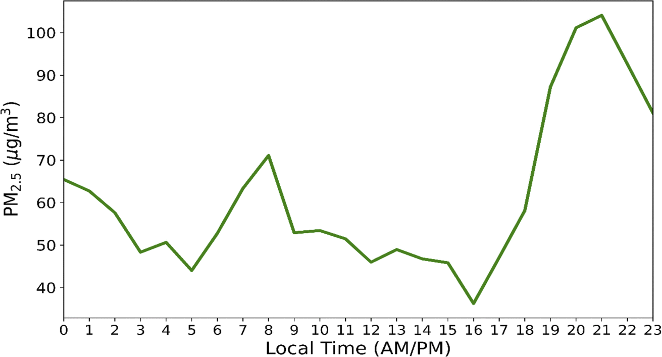

Fig. 2 Hourly profile of PM_2.5 at the U.S. Embassy site in Ouaga 2000, averaged for the year 2022.

Two peaks with different magnitudes were observed, one in the morning and one in the evening. The evening peak was higher with PM_2.5 concentrations at about 105 μg m⁻³ while the morning peak was lower with PM_2.5 concentrations at about 70 μg m⁻³. The morning peak was observed between 5:00 am and 9:00 am, and the evening peak was between 4:00 pm and 11:00 pm. The morning peak is likely due to morning vehicular traffic when people are going to work, and the evening peak is likely due to evening vehicular traffic when people return home after work. Cooking activities in the morning and evening also contribute to these peaks. Nana et al.²⁰ and Ouarma et al.¹⁹ observed similar peaks in administrative sites in Ouagadougou. These peaks are also similar to those observed by McFarlane et al.⁴⁶ in Kinshasa-Brazzaville and Bahino et al.⁴⁷ in Accra and Abidjan. Govender et al.⁴⁸ also found that PM_2.5 concentrations increased during early mornings and late afternoons in the Vaal Triangle Area of South Africa. The high concentrations of PM_2.5 in Ouagadougou in the evening is very likely due to the dynamics of the boundary layer (BL), which produces high dilution rates during the day and low dilution rates after sunset.⁴⁹ Fig. S2† illustrates the temporal changes between weekends and weekdays in Ouagadougou. PM_2.5 concentrations increase from Friday to Monday, followed by a decrease from Monday to Friday. Saturdays, Sundays, and Mondays consistently exhibit the highest pollution levels in the city, with PM_2.5 concentrations exceeding 65 μg m⁻³. This trend could be attributed to increased weekend traffic associated with leisure activities, shopping, and social events, resulting in higher vehicle emissions, though further activity data are needed. Elevated PM_2.5 levels on Mondays may stem from accumulated emissions over the weekend and heightened commuter traffic as the workweek begins. Notably, Saturdays in Ouagadougou are not considered full weekends, with work activities extending until 2 pm, which contributes to lower pollution levels compared to Sundays and Mondays, as depicted in Fig. S2.†

Fig. S3† presents an analysis of the potential source regions and contributions of PM_2.5 using Trajstat models and the Hybrid Single-Particle Lagrangian Integrated Trajectory (HYSPLIT) model, developed by the National Oceanic and Atmospheric Administration's (NOAA) Air Resources Laboratory (ARL).^50,51 We examined HYSPLIT back trajectories with meteorological data from the Global Data Assimilation System (GDAS) for extremely polluted days (hourly PM_2.5 concentrations greater than 350 μg m⁻³ and daily mean PM_2.5 concentrations greater than 200 μg m⁻³) in Ouagadougou. These days include January 28, February 7, March 13, 14, 19, and December 17. Back trajectories were calculated for 24 hour periods at three receptor heights (500 m, 1000 m, and 1500 m). The analysis reveals that on most of the extremely polluted days, the wind fields at these different heights predominantly originated from the east and northeast, extending to regions as far as Niger and northern Nigeria. An exception was noted on January 28, when back trajectories arriving at 500 m originated from the south. The West African region is influenced by dust from the northeast, where the Sahara Desert is located,^19,47 suggesting that the dust likely originated from the Sahara Desert but was slightly redirected by atmospheric dynamics.⁵² This is also consistent with the conditional bivariate analysis in Fig. S4,† which shows that wind from the east and north has some association with high PM_2.5 concentrations. These insights underscore the influence of meteorological conditions on PM_2.5 levels in Ouagadougou.

3.3 Correlation between observed PM_2.5 and corrected satellite weather parameters at the U.S. Embassy site in Ouaga 2000

Table 3 shows the correlation between surface PM_2.5 and AOD and corrected satellite data at the U.S. Embassy site in Ouaga 2000.

Table 3 Summary of the Pearson correlation coefficients between PM_2.5 and AOD and corrected satellite weather parameters at the U.S. Embassy site in Ouaga 2000

Parameters	r
AOD-PM2.5	0.72
Relative humidity-PM2.5	−0.55
Temperature-PM2.5	0.11
Precipitation-PM2.5	−0.26
Wind speed-PM2.5	−0.04
Wind direction-PM2.5	−0.33

---

PM_2.5 shows a weak negative correlation (r = −0.26) with CHIRPS precipitation. The negative correlation means that as precipitation increases, PM_2.5 decreases and vice versa. Wet deposition (not in the dry season) serves as the primary sink for atmospheric particulate matter, hence increases in precipitation result in a decline in particle concentrations.^53,54 The weak correlation means that most of the variations in PM_2.5 are not directly explained by precipitation. All the Era5-Land variables showed a negative correlation with surface PM_2.5 except temperature, which showed a positive correlation. Relative humidity had the strongest negative correlation (r = −0.55) followed by wind direction (r = −0.33) and wind speed (r = −0.04). The negative correlations imply that an increase in any of these variables will result in a decrease in PM_2.5.⁵⁵ High Relative humidity leads to hygroscopic growth of PM_2.5, which can increase mass and increase deposition rates similar to wet deposition by precipitation hence decreasing the concentrations of PM_2.5.^19,56 However, it is worth noting that high relative humidity can also lead to more hydroxyl radical (OH) driven by sunlight in Ouagadougou and more aqueous formation of aerosols.⁵⁴ Low wind speed leads to a stagnant atmosphere favoring PM_2.5 accumulation.⁵⁷

In contrast, high wind speeds promote PM_2.5 dissipation. High wind speeds can generate and transport dust. Similarly, the direction of the wind can determine the concentration of PM_2.5. If the wind direction is away from an area with PM_2.5 sources, the PM_2.5 particles are transported away from that area, resulting in lower PM_2.5 concentrations in that area and hence a negative correlation.⁵⁷ From the conditional bivariate analysis of the relationship between wind speed, wind direction, and PM_2.5 concentrations displayed in Fig. S4,† slow-moving winds (less than 1.5 m s⁻¹) from the north and medium-moving winds (1.5–3.0 m s⁻¹) from the east and north are associated with high PM_2.5 concentrations. Conversely, high-moving winds greater than 4 m s⁻¹ are associated with lower PM_2.5 concentrations. However, the weak correlations of the parameters with PM_2.5 imply that most of the changes in PM_2.5 are not directly explained by the parameters and their relationship might be more complex. The correlation between temperature and surface PM_2.5 was 0.11. An increase in temperature leads to some increase in PM_2.5 concentrations.^53,54 However, the weak correlation observed in our findings indicates that most of the variations in PM_2.5 are not directly explained by temperature.

3.4 Statistical regression and non-linear machine learning models

Fig. 3 shows the performance of statistical regression models and non-linear machine learning models at the U.S. Embassy site (Ouaga 2000).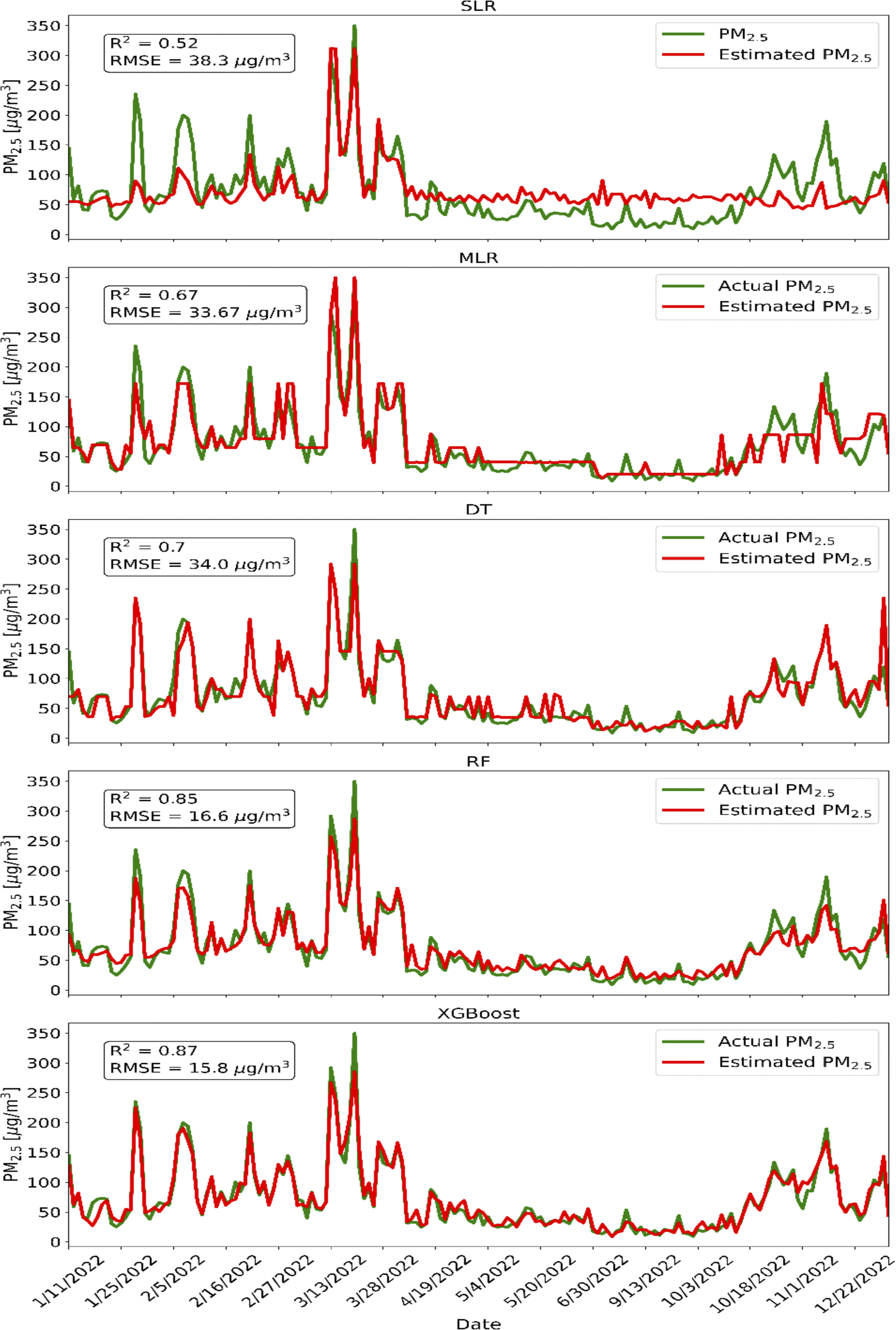

Fig. 3 Performance of the statistical regression models and the non-linear machine learning models at the U.S. Embassy site (Ouaga 2000).

The SLR model developed is:

PM_2.5 = 75.61 × AOD + 38.36 (8)

The model has an R² of 0.52 after a five-fold cross-validation, indicating that MODIS AOD explains about half of the variations in surface PM_2.5. The RMSE of the model after cross-validation was 38.3 μg m⁻³ and the significance F was 1.23 × 10⁻²² (less than α = 0.05). These findings are similar to those of by Van Donkelaar et al.⁵⁸ They obtained R² of 0.59 between MODIS AOD and PM_2.5 over Eastern China. Wang and Christopher²² obtained an R² of 0.49 at seven locations in Jefferson County, Alabama. Koelemeijer et al.⁵⁹ also obtained an R² of 0.36 between AOD and PM_2.5 at some locations in Europe.

The MLR model developed is:

PM_2.5 = 174.11 + 69.27 × AOD − 1.65 × T − 1.00 × RH − 14.04 × WS − 1.54 × Precip − 0.08 × WD (9)

The MLR model has an R² of 0.67 and an RMSE of 33.7 μg m⁻³ after a five-fold cross-validation with a significance F of 8.85 × 10⁻³⁰ (less than α = 0.05). One explanation for this is that the inclusion of meteorological parameters leads to better prediction of surface PM_2.5, the MLR model explains 0.67 of the variations in surface PM_2.5 with a smaller RMSE compared to the SLR model. These findings are consistent with the findings of Tian and Chen.²⁹ Their regression model explained 0.65 of the variations in observed PM_2.5.

The decision tree model explains 0.70 of the variations in surface PM_2.5 with an RMSE of 34.0 μg m⁻³ after a five-fold cross-validation. The decision tree model performed the least in the non-linear models. The decision tree model uses a single tree and offers less hyperparameter tuning and hence was not able to better capture complex relationships. The random forest model explains 0.85 of the variations in observed PM_2.5 with an RMSE of 16.6 μg m⁻³ after a five-fold cross-validation. McFarlane et al.⁶⁰ used a random forest model for correcting low-cost sensors PM_2.5 data in Kampala, Uganda, and had a similar performance (R² of 0.86). The XGBoost model explains 0.87 of the variations of surface PM_2.5 with a lower RMSE of 15.8 μg m⁻³ after a five-fold cross-validation outperforming all the models. XGBoost offers more hyperparameters tuning and this results in its outstanding performance. These findings clearly show that non-linear models perform better than linear models in estimating surface PM_2.5.^61,62

In all the models, MODIS AOD is the most important feature in PM_2.5 estimation, followed by relative humidity and temperature as shown in Fig. S6.† Precipitation is a less important parameter in the models' estimation. This means that the impact of precipitation in explaining the variability of PM_2.5 is less significant than that of AOD, relative humidity, temperature, wind speed, and wind direction.

Emission source and meteorological attribution data in Ouagadougou is scarce. A study by Lindén¹⁸ found that extremely stable nocturnal atmospheric conditions occurred on 80% of the days at the beginning of the dry season in Ouagadougou. The frequent occurrence of these stable conditions and the intra-urban thermal wind fields result in limited ventilation and dispersion of urban pollutants.¹⁸ Increased air pollution concentrations during stable conditions with low wind speeds have been identified as a factor in air quality issues in semi-arid African cities.⁶³ We confirm this is also the case in our dataset in the conditional bivariate analysis of the relationship between wind speed, wind direction, and PM_2.5 concentrations in Fig. S4† where low to moderate wind speeds tend to be associated with high PM_2.5. Lindén¹⁸ also highlighted that key pollution sources include road dust re-suspension, transported dust, traffic emissions, and biomass burning. In developing countries, many households rely on biomass burning and using open fires, often in poorly ventilated areas, leading to severe air pollution.⁶⁴ While biomass is more commonly used in rural areas, it is also prevalent in low-income urban areas.⁶³ A study on household energy in Ouagadougou, Burkina Faso, found that over 80% of urban residents used biomass as their primary energy source.⁶⁵ Additionally, in developing countries, traffic often consists of many old, poorly maintained vehicles and numerous two-stroke engines, which are highly polluting.^20,21

3.5 Semi-supervised XGBoost model

Fig. 4 shows the performance of the semi-supervised XGBoost model.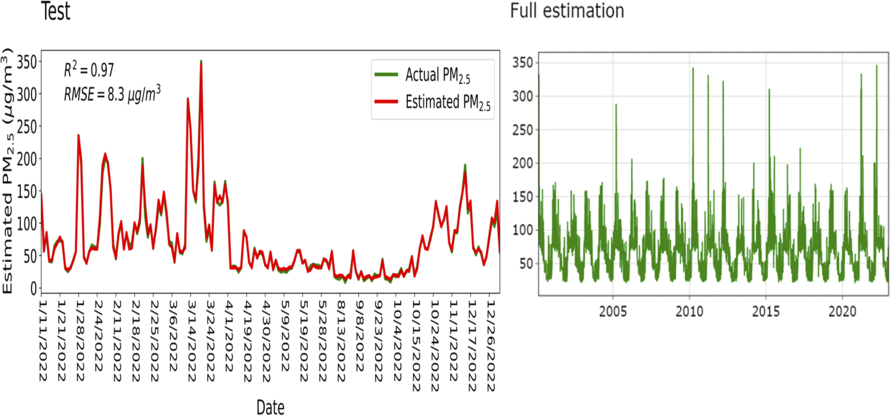

Fig. 4 Performance of the semi-supervised XGBoost model.

The model has an R² of 0.97, and an RMSE of 8.3 μg m⁻³ after a five-fold cross-validation, indicating that the model explains 0.97 of the variations in PM_2.5 with the lowest RMSE. The model is validated using an independent dataset for the period of August 2023 to October 2023 from the tapered element oscillating microbalance (TEOM 1400a, a federal equivalent method gravimetric PM_2.5 monitor)⁶⁶ located at Université Joseph Ki-Zerbo in Ouagadougou. The model effectively explains 91% of the measurements recorded by the TEOM (R² = 0.91) with minimal error (RMSE = 3.70 μg m⁻³) as shown in Fig. S8.† These results significantly enhance the reliability and confirm the generalizability of the model. These findings are similar to those of Bougoudis et al.⁶⁷ because their semi-supervised ANN model explained approximately 0.9 of the variations in air pollutants in Athens, Greece. Similarly, the semi-supervised k-nearest neighbours (KNN) model proposed by Zhao et al.⁶⁸ in China had an R² of 0.97. Fig. 4 also shows the estimation of PM_2.5 by the model on the whole data (labeled and unlabeled) after testing. It is observed that in the whole city, days in the dry season are associated with high PM_2.5 concentrations (2 to 22 times higher than the WHO 24 hour guideline of 15 μg m⁻³), and days in the rainy season are associated with low PM_2.5 concentrations (2 to 4 times higher than the WHO 24 hour guideline of 15 μg m⁻³), and the same trend is observed every year. This trend is similar in other Sahelian cities that share the same climatic conditions and experience similar Harmattan winds as Ouagadougou. Garrison et al.⁶⁹ found that the mean 24 hour PM_2.5 concentrations in Bamako are 43 μg m⁻³ (2.9 times higher than the WHO 24 hour guideline of 15 μg m⁻³) during the rainy season and up to 500 μg m⁻³ (33.3 times higher than the WHO guideline of 15 μg m⁻³) during the dry season. In Dakar, the mean 24 hour PM_2.5 concentrations are 26 μg m⁻³ (1.7 times higher than the WHO guideline of 15 μg m⁻³) during the rainy season and up to 330 μg m⁻³ (22 times higher than the WHO guideline of 15 μg m⁻³) during the dry season.⁷⁰ This implies that aside from internal sources of PM_2.5 pollution within these cities, the Harmattan winds are a significant external contributor to the high levels of PM_2.5 pollution. This natural phenomenon, combined with local pollution sources, results in the extremely high PM_2.5 concentrations observed during the dry season.¹⁹

3.6 Average yearly and monthly trend of estimated PM_2.5 in Ouagadougou

Fig. 5 shows the average yearly and monthly trend of estimated PM_2.5 in Ouagadougou.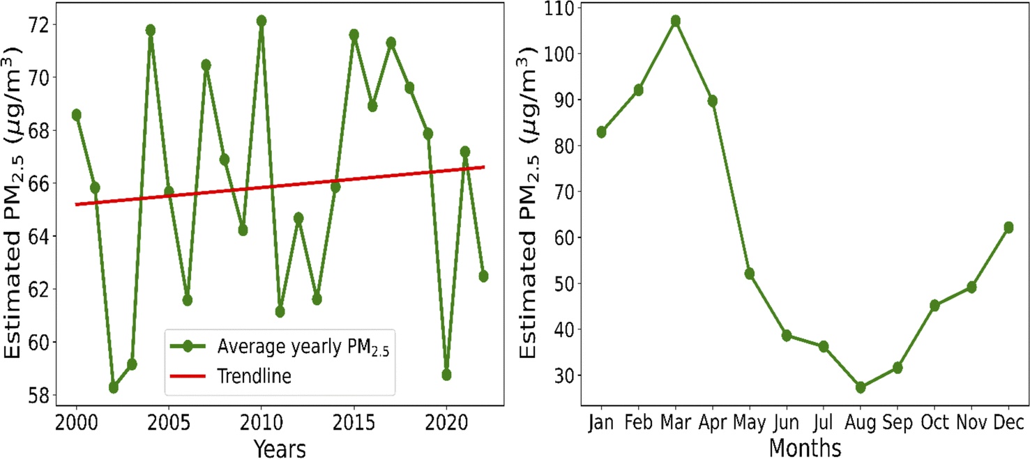

Fig. 5 Average yearly and monthly trend of estimated PM_2.5 in Ouagadougou.

The yearly trend of PM_2.5 in the city is not direct. The PM_2.5 levels fluctuate irregularly, showing variations that are not easily predictable or following a simple upward or downward trend throughout the years in the study period. A direct trend means that PM_2.5 levels show a predictable or linear increase, decrease, or stability over the years in the study period without significant fluctuations or irregularities. The yearly PM_2.5 trend increases and decreases but, in general, there is a slight increasing trend which is not significant (p-value of 0.65 > 0.05). The average annual estimated PM_2.5 concentrations range from 58.2 μg m⁻³ to 72.1 μg m⁻³, which is 11 to 14 times higher than the WHO guidelines of 5 μg m⁻³ annually and 6 to 8 times higher than the U.S. Environmental Protection Agency (EPA) guidelines of 9 μg m⁻³ annually. Significant increases in the trend were observed in 2004, 2010, and 2015 whilst significant decreases were observed in 2002, 2003, and 2020. Interannual variability and weather can affect year-to-year changes in PM_2.5. Generally, the city is growing in population and economic activity,³³ which can lead to enhanced PM_2.5 concentrations. In 2020, however, when there was a lockdown due to COVID-19, it was observed that the PM_2.5 trend decreased significantly. This is because of the reduction in industrial activities and heavy traffic due to the lockdown. However, the overall trend largely depends on the intensity of dust from the Sahara Desert and the variability of weather conditions²¹ as well as the intensity of emissions from unpaved roads, heavy traffic, and industrial activities in a given year.^19,20,63 March has the highest PM_2.5 concentrations with an average of 107 μg m⁻³ because the dust from the Sahara Desert transported by Harmattan winds reaches its peak in March. Dust from unpaved roads and biomass burning are also major contributors to higher concentrations in the dry season.²⁰ August has the lowest PM_2.5 concentrations with an average of 16 μg m⁻³, attributed to the significant precipitation during the month. These findings align with those of Awokola et al.,⁷¹ who observed elevated PM_2.5 levels in March and April and lower PM_2.5 levels in August in Balkuy, a town in the same region as Ouagadougou in Burkina Faso. Ouarma et al.¹⁹ also found mean PM_2.5 levels of 22 μg m⁻³ during the rainy season months and 87 μg m⁻³ during the dry season months in 2019 in Ouagadougou. The increased rainfall in August leads to more particle deposition and reduced urban activities and road dust, contributing to cleaner air.

3.7 Spatial distribution of PM_2.5 concentrations in Ouagadougou

Fig. 6 shows the spatial distribution of estimated PM_2.5 concentrations in rainy and dry seasons of 2000–2009 and 2012–2022 (excluding the COVID-19 year, 2020) and the difference between the two periods in Ouagadougou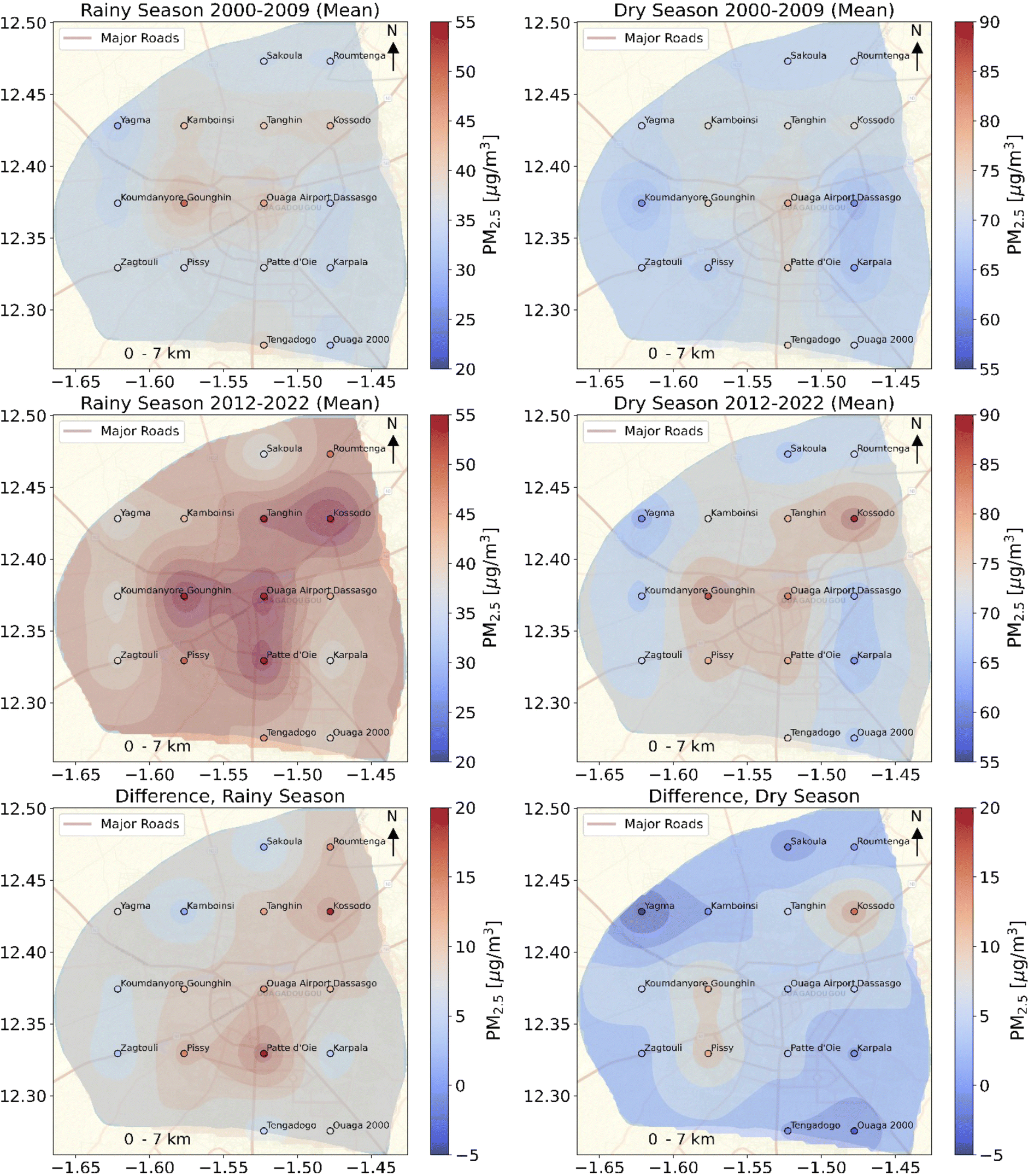

Fig. 6 Spatial distribution of estimated PM_2.5 concentrations in rainy and dry seasons of 2000–2009 and 2012–2022 (excluding the COVID-19 year, 2020) and the difference between the two periods in Ouagadougou.

The mean estimated PM_2.5 concentrations in all areas of the city in the rainy season of 2000–2009 were lower (between 30 μg m⁻³ and 40 μg m⁻³) except at Gounghin, Ouagadougou Airport, Tanghin, Kamboinsi, and Kossodo where the PM_2.5 concentrations were slightly above 40 μg m⁻³. Wet deposition in the rainy season removes PM_2.5 particles from the atmosphere.^19,53,56 Also, rainfall dampens the ground, reducing the amount of dust and other particles that can be resuspended into the air through wind or human activities.⁷² Additionally, the rainy season often coincides with increased vegetation growth, which can help trap particulates and prevent them from becoming airborne.⁷³

In the dry season of the same period, the PM_2.5 concentrations were between 65 μg m⁻³ and 70 μg m⁻³ except in Ouagadougou Airport, Patte d'Oie, Gounghin, Tanghin, Kamboinsi, Kossodo, and Tengadogo where the PM_2.5 concentrations were slightly higher, between 70 μg m⁻³ and 75 μg m⁻³. The slightly higher mean PM_2.5 concentrations in these areas in both seasons could depict emissions from vehicles. The high PM_2.5 concentrations in every area of the city in the dry season are mainly due to the dust transported from the Sahara Desert by the Harmattan winds from November to March^18,20 and also dust from unpaved roads.²⁰ Also, frequent atmospheric stability caused by temperature inversions during the early dry season favors the accumulation of air pollutants.¹⁸ Additionally, during the dry season, there is an increase in open burning of household waste, further exacerbating air pollution levels.⁷⁴ The mean estimated PM_2.5 concentrations in the rainy season of 2012–2022 were high between 40 μg m⁻³ and 45 μg m⁻³ in all areas except in Gounghin, Kossodo, Ouagadougou Airport, Patte d'Oie, and Tanghin where the mean PM_2.5 concentrations were between 50 μg m⁻³ and 55 μg m⁻³. The mean estimated PM_2.5 concentrations in Yagma, Koumdanyore, Zagtouli, Ouaga 2000, Sakoula, and Roumtenga in the dry season of the same period were between 60 μg m⁻³ and 70 μg m⁻³ whereas in Ouagadougou Airport, Patte d'Oie, Gounghin, Tanghin, and Kossodo, the estimated PM_2.5 concentrations were between 80 μg m⁻³ and 90 μg m⁻³. Ouagadougou Airport, Patte d'Oie, Kamboinsi, and Tanghin are home to many commercial activities with high volumes of traffic. Kossodo and Gounghin are the most established industrial zones in the city with several gas-oil power plants, cement and brick factories, metal processing plants, and textile manufacturing units.³² Additionally, these areas are frequented by heavy trucks fueled by diesel for transporting raw materials and finished products; hence, higher levels of PM_2.5 in these areas. For Patte d'Oie, Kossodo, Ouagadougou Airport, Pissy, Tanghin, Dassasgo, Gounghin, and Roumtenga, estimated PM_2.5 concentrations in the rainy season increased to about 10–20 μg m⁻³ in 2012–2022 from their levels in 2000–2009. For Kossodo, Gounghin, and Pissy, estimated PM_2.5 concentrations in the dry season increased to about 10–15 μg m⁻³. PM_2.5 concentrations in Yagma, Ouaga 2000, Sakoula, and Tengadogo in the dry season decreased to about 3–5 μg m⁻³ compared to their levels in 2000–2009. These decreases may be attributed to improvements in the number of paved roads in these areas.

4. Conclusions

PM_2.5 concentrations in Ouagadougou were estimated from satellite aerosol optical depth and meteorological parameters using different models in this study. In all the models, AOD was the most important parameter for estimating PM_2.5 in the city. However, the addition of meteorological parameters increased the performance of the models and hence their ability to explain the variations in surface PM_2.5 indicating that meteorological parameters influence the variability of PM_2.5. XGBoost outperforms all the supervised models and is upgraded into a semi-supervised XGBoost model by incorporating a semi-supervised algorithm. The semi-supervised XGBoost can explain the variability of PM_2.5 in the city indicating that with the addition of the large amount of unlabeled data, the variability of surface PM_2.5 in the city can be captured. The semi-supervised XGBoost model reveals that the estimated PM_2.5 concentrations in the city are 2 to 4 times higher than the WHO 24 hour guideline of 15 μg m⁻³ in the rainy season and 2 to 22 times higher than the WHO 24 hour guideline in the dry season. The industrial areas (Gounghin and Kossodo) and areas around the center of the city are the major polluting areas of the city. This research has provided information on PM_2.5 concentrations in Ouagadougou that would help in epidemiological studies, city planning, and air quality decision-making. Converting satellite AOD to surface PM_2.5 is very common in places where ground measurements of PM_2.5 are lacking. In areas like Ghana, where there are more ground measurements,^75,76 this method would work even more better and the biases between the estimated and observed PM_2.5 concentrations would be reduced.

Data availability

NASA data is available here: https://worldview.earthdata.nasa.gov/ and US Embassy data is available here: https://www.airnow.gov/international/us-embassies-and-consulates/.

Author contributions

JAA, DMW, KOH, BN: led conceptualization, supervision, secured funding, provided resources, curated data, developed methodology, validated results, and reviewed and edited draft. JAA: conducted formal analysis, developed models, visualized data, and wrote an original draft.

Conflicts of interest

The authors declare no conflicts of interest.

Acknowledgements

We thank the German Federal Ministry of Education and Research (BMBF) and the West African Science Service Center on Climate Change and Adapted Land Use (WASCAL) for providing funds for this study. We also thank the U.S. Embassy in Ouagadougou for guaranteeing the caliber of BAM data that is accessible on the Airnow database. We thank the Agence Nationale de la Météorologie du Burkina Faso (ANAM-BF) for providing us with meteorological data. This work was also supported by National Science Foundation Office of International Science and Engineering (OISE) Award Number 2020677.

Notes and references

1. S. Fisher, D. C. Bellinger, M. L. Cropper, P. Kumar, A. Binagwaho, J. B. Koudenoukpo, Y. Park, G. Taghian and P. J. Landrigan, Lancet Planet Health, 2021, 5, e681–e688.
2. H. Carvalho, Lancet Planet Health, 2021, 5, e760–e761.
3. World Health Organization (WHO), WHO global air quality guidelines: Particulate matter (PM_2.5 and PM₁₀), ozone, nitrogen dioxide, sulfur dioxide and carbon monoxide, 2021, pp. 1–360.
4. R. Burnett, H. Chen, M. Szyszkowicz, N. Fann, B. Hubbell, C. A. Pope, J. S. Apte, M. Brauer, A. Cohen, S. Weichenthal, J. Coggins, Q. Di, B. Brunekreef, J. Frostad, S. S. Lim, H. Kan, K. D. Walker, G. D. Thurston, R. B. Hayes, C. C. Lim, M. C. Turner, M. Jerrett, D. Krewski, S. M. Gapstur, W. R. Diver, B. Ostro, D. Goldberg, D. L. Crouse, R. V. Martin, P. Peters, L. Pinault, M. Tjepkema, A. Van Donkelaar, P. J. Villeneuve, A. B. Miller, P. Yin, M. Zhou, L. Wang, N. A. H. Janssen, M. Marra, R. W. Atkinson, H. Tsang, T. Q. Thach, J. B. Cannon, R. T. Allen, J. E. Hart, F. Laden, G. Cesaroni, F. Forastiere, G. Weinmayr, A. Jaensch, G. Nagel, H. Concin and J. V. Spadaro, Proc. Natl. Acad. Sci. U. S. A., 2018, 115, 9592–9597.
5. A. J. Cohen, M. Brauer, R. Burnett, H. R. Anderson, J. Frostad, K. Estep, K. Balakrishnan, B. Brunekreef, L. Dandona, R. Dandona, V. Feigin, G. Freedman, B. Hubbell, A. Jobling, H. Kan, L. Knibbs, Y. Liu, R. Martin, L. Morawska, C. A. Pope, H. Shin, K. Straif, G. Shaddick, M. Thomas, R. van Dingenen, A. van Donkelaar, T. Vos, C. J. L. Murray and M. H. Forouzanfar, Lancet, 2017, 389, 1907–1918.
6. C. Song, J. He, L. Wu, T. Jin, X. Chen, R. Li, P. Ren, L. Zhang and H. Mao, Environ. Pollut., 2017, 223, 575–586.
7. Y. F. Xing, Y. H. Xu, M. H. Shi and Y. X. Lian, J. Thorac. Dis., 2016, 8, E69.
8. D. Y. H. Pui, S. C. Chen and Z. Zuo, Particuology, 2014, 13, 1–26.
9. M. L. Bell, F. Dominici, K. Ebisu, S. L. Zeger and J. M. Samet, Environ. Health Perspect., 2007, 115, 989–995.
10. S. Feng, D. Gao, F. Liao, F. Zhou and X. Wang, Ecotoxicol. Environ. Saf., 2016, 128, 67–74.
11. A. J. Cohen, H. R. Anderson, B. Ostro, K. D. Pandey, M. Krzyzanowski, N. Künzli, K. Gutschmidt, A. Pope, I. Romieu, J. M. Samet and K. Smith, J. Toxicol. Environ. Health, Part A, 2005, 68, 1301–1307.
12. J. H. Seinfeld, S. N. Pandis and Atmospheric Chemistry and Physics: From Air Pollution to Climate Change, Wiley, 2006.
13. G. Rushingabigwi, P. Nsengiyumva, L. Sibomana, C. Twizere and W. Kalisa, Atmos. Environ., 2020, 224, 117319.
14. USEPA, Particulate Matter (PM) Basics, 2016.
15. J. Li, X. Han, M. Jin, X. Zhang and S. Wang, Environ. Int., 2019, 128, 46–62.
16. L. Han, W. Zhou, W. Li and L. Li, Environ. Pollut., 2014, 194, 163–170.
17. C.-S. Liang, F.-K. Duan, K.-B. He and Y.-L. Ma, Environ. Int., 2015, 86, 150–170.
18. J. Lindén, Int. J. Bioclimatol. Biometeorol., 2011, 31, 605–620.
19. I. Ouarma, B. Nana, K. Haro, A. Béré and J. Koulidiati, J. Geosci. Environ. Prot., 2020, 8, 119–138.
20. B. Nana, O. Sanogo, P. W. Savadogo, T. Daho, M. Bouda and J. Koulidiati, FUTY J. Environ., 2012, 7, 1–18.
21. J. Lindén, S. Thorsson, J. Boman and B. Holmer, Urban climate and air pollution in Ouagadougou, Doctoral thesis, University of Gothenburg, Burkina Faso, 2012.
22. J. Wang and S. A. Christopher, Geophys. Res. Lett., 2003, 30, 2095.
23. A. van Donkelaar, R. V. Martin, M. Brauer, R. Kahn, R. Levy, C. Verduzco and P. J. Villeneuve, Environ. Health Perspect., 2010, 118, 847–855.
24. T. Xue, Y. Zheng, G. Geng, B. Zheng, X. Jiang, Q. Zhang and K. He, RemS, 2017, 9, 221.
25. A. Van Donkelaar, R. V. Martin, M. Brauer and B. L. Boys, Environ. Health Perspect., 2015, 123, 135–143.
26. S. Zhai, D. J. Jacob, J. F. Brewer, K. Li, J. M. Moch, J. Kim, S. Lee, H. Lim, H. C. Lee, S. K. Kuk, R. J. Park, J. I. Jeong, X. Wang, P. Liu, G. Luo, F. Yu, J. Meng, R. V. Martin, K. R. Travis, J. W. Hair, B. E. Anderson, J. E. Dibb, J. L. Jimenez, P. Campuzano-Jost, B. A. Nault, J. H. Woo, Y. Kim, Q. Zhang and H. Liao, Atmos. Chem. Phys., 2021, 21, 16775–16791.
27. X. Jin, A. M. Fiore, G. Curci, A. Lyapustin, K. Civerolo, M. Ku, A. Van Donkelaar and R. V. Martin, Atmos. Chem. Phys., 2019, 19, 295–313.
28. M. S. Hammer, A. Van Donkelaar, C. Li, A. Lyapustin, A. M. Sayer, N. C. Hsu, R. C. Levy, M. J. Garay, O. V. Kalashnikova, R. A. Kahn, M. Brauer, J. S. Apte, D. K. Henze, L. Zhang, Q. Zhang, B. Ford, J. R. Pierce and R. V. Martin, Environ. Sci. Technol., 2020, 54, 7879–7890.
29. J. Tian and D. Chen, Remote Sens. Environ., 2010, 114, 221–229.
30. Z. Wang, L. Chen, J. Tao, Y. Zhang and L. Su, Remote Sens. Environ., 2010, 114, 50–63.
31. V. Etyemezian, M. Tesfaye, A. Yimer, J. C. Chow, D. Mesfin, T. Nega, G. Nikolich, J. G. Watson and M. Wondmagegn, Atmos. Environ., 2005, 39, 7849–7860.
32. B. Gouba, M. H. Sirima and B. Naon, Environ. Pollut., 2021, 10, 46.
33. D. D. Somda, Inventaire d'émissions de polluants atmosphériques issus du trafic routier à Ouagadougou (Burkina Faso). – References, Scientific Research Publishing, 2018, https://www.scirp.org/reference/referencespapers.aspx?referenceid=2861701, (accessed 6 April 2023).
34. P. Mateus, V. B. Mendes, S. M. Plecha, S. Bonafoni and I. D. Luiz, Remote Sens., 2021, 13, 2179.
35. J. A. Engel-Cox, C. H. Holloman, B. W. Coutant and R. M. Hoff, Atmos. Environ., 2004, 38, 2495–2509.
36. W. Song, H. Jia, J. Huang and Y. Zhang, Remote Sens. Environ., 2014, 154, 1–7.
37. L. Zhang, P. Liu, L. Zhao, G. Wang, W. Zhang and J. Liu, Atmos. Pollut. Res., 2021, 12, 328–339.
38. H. Jiang, X. Wang and C. Sun, Atmosphere, 2022, 13, 1744.
39. S.-Y. Kim, S.-J. Yi, Y. S. Eum, H.-J. Choi, H. Shin, H. G. Ryou and H. Kim, Environ. Health Toxicol., 2014, 29, e2014012.
40. J. Liu, B. Zheng and J. Fan, Lecture Notes in Civil Engineering, 2023, vol. 211, pp. 1158–1169.
41. V. Marx, Nat. Methods, 2022, 19(4), 403–407.
42. P. Ozer, A. Dembele, S. S. Yameogo, E. Hut and F. de Longueville, World Dev. Perspect., 2022, 25, 100393.
43. K. Du Plessis and J. Kibii, J. S. Afr. Inst. Civ. Eng., 2021, 63, 43–54.
44. A. D. Assamnew and G. Mengistu Tsidu, Int. J. Bioclimatol. Biometeorol., 2023, 43, 17–37.
45. S. Gleixner, T. Demissie and G. T. Diro, Atmosphere, 2020, 11, 996.
46. C. McFarlane, G. Raheja, C. Malings, E. K. E. Appoh, A. F. Hughes and D. M. Westervelt, ACS Earth Space Chem., 2021, 5, 2268–2279.
47. J. Bahino, M. Giordano, M. Beekmann, V. Yoboué, A. Ochou, C. Galy-Lacaux, C. Liousse, A. Hughes, J. Nimo, F. Lemmouchi, J. Cuesta, A. K. Amegah and R. Subramanian, Environ. Sci.: Atmos., 2024, 4, 468–487.
48. K. Govender and V. Sivakumar, Clean Air J., 2019, 29(2) DOI:10.17159/CAJ/2019/29/2.7578.
49. J. Lee, J. W. Hong, K. Lee, J. Hong, E. Velasco, Y. J. Lim, J. B. Lee, K. Nam and J. Park, Bound.–Layer Meteorol., 2019, 172, 435–455.
50. R. R. Draxler, S. Spring, U. S. A. Maryland and G. D. Hess, Aust. Meteorol. Mag., 1998, 47, 295–308.
51. A. F. Stein, R. R. Draxler, G. D. Rolph, B. J. B. Stunder, M. D. Cohen and F. Ngan, Bull. Am. Meteorol. Soc., 2015, 96, 2059–2077.
52. D. Francis, R. Fonseca, N. Nelli, J. Cuesta, M. Weston, A. Evan and M. Temimi, Geophys. Res. Lett., 2020, 47(24) DOI:10.1029/2020GL090102.
53. A. P. K. Tai, L. J. Mickley and D. J. Jacob, Atmos. Chem. Phys., 2012, 12, 11329–11337.
54. D. M. Westervelt, L. W. Horowitz, V. Naik, A. P. K. Tai, A. M. Fiore and D. L. Mauzerall, Atmos. Environ., 2016, 142, 43–56.
55. N. Islam, T. R. Toha, M. M. Islam and T. Ahmed, Aerosol Air Qual. Res., 2023, 23(1) DOI:10.4209/AAQR.220082.
56. C. Lou, H. Liu, Y. Li, Y. Peng, J. Wang and L. Dai, Environ. Monit. Assess., 2017, 189, 1–16.
57. D. Sirithian and P. Thanatrakolsri, Air, Soil Water Res., 2022, 15 DOI:10.1177/11786221221117264.
58. A. van Donkelaar, R. V. Martin, M. Brauer, R. Kahn, R. Levy, C. Verduzco and P. J. Villeneuve, Environ. Health Perspect., 2010, 118, 847–855.
59. R. B. A. Koelemeijer, C. D. Homan and J. Matthijsen, Atmos. Environ., 2006, 40, 5304–5315.
60. C. McFarlane, P. K. Isevulambire, R. S. Lumbuenamo, A. M. E. Ndinga, R. Dhammapala, X. Jin, V. F. McNeill, C. Malings, R. Subramanian and D. M. Westervelt, Aerosol Air Qual. Res., 2021, 21(7) DOI:10.4209/AAQR.200619.
61. M. Z. Joharestani, C. Cao, X. Ni, B. Bashir and S. Talebiesfandarani, Atmosphere, 2019, 10, 373.
62. K. Kumar and B. P. Pande, Int. J. Environ. Sci. Technol., 2022, 1–16.
63. J. Boman, J. Lindén, S. Thorsson, B. Holmer and I. Eliasson, X-Ray Spectrom., 2009, 38, 354–362.
64. D. G. Fullerton, N. Bruce and S. B. Gordon, Trans. R. Soc. Trop. Med. Hyg., 2008, 102, 843–851.
65. V. Zoma, Transport routier et pollution de l’air dans la ville de Ouagadougou, Revue Ivoirienne de Sociologie et de Sciences Sociales (RISS), 2022, vol. 1(9).
66. ThermoFisher, Operating Manual, TEOM Series 1400a Ambient Particulate (PM-10) Monitor, 2008.
67. I. Bougoudis, K. Demertzis, L. Iliadis, V. D. Anezakis and A. Papaleonidas, Commun. Comput. Inf. Sci., 2016, 629, 51–63.
68. Y. Zhao, L. Wang, N. Zhang, X. Huang, L. Yang and W. Yang, Atmosphere, 2023, Vol. 14, 143.
69. V. H. Garrison, M. S. Majewski, L. Konde, R. E. Wolf, R. D. Otto and Y. Tsuneoka, Sci. Total Environ., 2014, 500–501, 383–394.
70. D. Sarr, B. Diop, A. K. Farota, A. Sy, A. D. Diop, M. Wade and A. B. Diop, J. Pollut. Eff. Control, 2018, 6(3) DOI:10.4172/2375-4397.1000230.
71. B. Awokola, G. Okello, O. Johnson, R. Dobson, A. R. Ouédraogo, B. Dibba, M. Ngahane, C. Ndukwu, C. Agunwa, D. Marangu, H. Lawin, I. Ogugua, J. Eze, N. Nwosu, O. Ofiaeli, P. Ubuane, R. Osman, E. Awokola, A. Erhart, K. Mortimer, C. Jewell and S. Semple, Atmosphere, 2022, 13, 1593.
72. I. Casotti Rienda and C. A. Alves, Atmos. Res., 2021, 261, 105740.
73. A. Diener and P. Mudu, Sci. Total Environ., 2021, 796 DOI:10.1016/J.SCITOTENV.2021.148605.
74. J. N. D. Gordon, K. R. Bilsback, M. N. Fiddler, R. P. Pokhrel, E. V. Fischer, J. R. Pierce and S. Bililign, Geohealth, 2023, 7, e2022GH000673.
75. G. Raheja, J. Nimo, E. K. E. Appoh, B. Essien, M. Sunu, J. Nyante, M. Amegah, R. Quansah, R. E. Arku, S. L. Penn, M. R. Giordano, Z. Zheng, D. Jack, S. Chillrud, K. Amegah, R. Subramanian, R. Pinder, E. Appah-Sampong, E. N. Tetteh, M. A. Borketey, A. F. Hughes and D. M. Westervelt, Environ. Sci. Technol., 2023, 57, 10708–10720.
76. C. Mcfarlane, G. Raheja, C. Malings, E. K. E. Appoh, A. F. Hughes and D. M. Westervelt, ACS Earth Space Chem., 2021, 5(9) DOI:10.1021/acsearthspacechem.1c00217.

---

Footnote

† Electronic supplementary information (ESI) available. See DOI: https://doi.org/10.1039/d4ea00057a

---