
 Open Access Article
 This Open Access Article is licensed under a Creative Commons Attribution-Non Commercial 3.0 Unported Licence
Pulse length dependence of photoelectron circular dichroism†
Han-gyeol
Lee
 *a,
Simon T.
Ranecky
a,
Sudheendran
Vasudevan
a,
Nicolas
Ladda
a,
Tonio
Rosen
a,
Sagnik
Das
a,
Jayanta
Ghosh
a,
Hendrike
Braun
a,
Daniel M.
Reich
b,
Arne
Senftleben
a and
Thomas
Baumert
*a
*a,
Simon T.
Ranecky
a,
Sudheendran
Vasudevan
a,
Nicolas
Ladda
a,
Tonio
Rosen
a,
Sagnik
Das
a,
Jayanta
Ghosh
a,
Hendrike
Braun
a,
Daniel M.
Reich
b,
Arne
Senftleben
a and
Thomas
Baumert
*a
aInstitut für Physik, Universität Kassel, Heinrich-Plett-Str. 40, 34132 Kassel, Germany. E-mail: hgyeol@uni-kassel.de; tbaumert@uni-kassel.de
bDahlem Center for Complex Quantum Systems and Fachbereich Physik, Freie Universität Berlin, Arnimallee 14, D-14195 Berlin, Germany
First published on 7th November 2022
Abstract
We investigate photoelectron circular dichroism (PECD) with coherent light sources whose pulse durations range from femtoseconds to nanoseconds. To that end, we employed an optical parametric amplifier, an ultraviolet optical pulse shaper, and a nanosecond dye laser, all centered around a wavelength of 380 nm. A multiphoton ionization experiment on the gas-phase chiral prototype fenchone found that PECD measured via the 3s intermediate resonance is about 15% and robust over five orders of magnitude of the pulse duration. PECD remains robust despite ongoing molecular dynamics such as rotation, vibration, and internal conversion. We used the Lindblad equation to model the molecular dynamics. Under the assumption of a cascading internal conversion, from the 3p to the 3s and further to the ground state, we estimated the lifetimes of the internal conversion processes in the 100 fs regime.
1 Introduction
Chiroptical spectroscopy on gas-phase molecules utilizing enantiomer-sensitive light–matter interaction is a promising research field under rapid development. Various essential topics and techniques such as circular dichroism (CD) in ion yield, photoelectron circular dichroism (PECD), microwave three-wave mixing, and Coulomb explosion imaging have been reviewed in, e.g.,1–5 Taking advantage of the interaction-free nature in the gas phase, novel approaches and results have been reported in recent years, for example, self-referencing ion yield CD measurements,6–8 PECD for fully fixed in space molecules,9 enantiomeric enrichment in a rotational level using microwave three-wave mixing,10 orientation-dependent circular dichroism at the single-molecule level,11 an optical centrifuge for enantioselective orientation12, and the demonstration of two different chiral sensitive high-harmonic spectroscopy techniques as purely optical methods.13Photoelectron circular dichroism (PECD), the forward–backward asymmetry of photoelectrons from chiral molecules ionized by circularly polarized light, has a special significance. The asymmetry lies along the propagation direction of the light which is on the order of 10%. From the very first theoretical prediction in 1976,14 it took about 25 years for the first experimental verification of PECD in the single-photon ionization of chiral molecules using synchrotron radiation.15,16 After another 10 years, the first table-top PECD experiment was demonstrated in the multiphoton ionization of chiral molecules using a femtosecond laser.17,18 Since then, many important details on the multiphoton PECD, e.g., its dependence on the pulse intensity and ellipticity,19–23 the enantiomeric excess of the target,23–25 or the intermediate electronic states involved in different multiphoton ionization schemes,22,26–31 have been studied. More over, very recent studies reported PECD measurements on a microjet of liquid chiral substance32 and in the photodetachment from anions.33
Theoretical approaches to describe the multiphoton PECD range from combined ab initio quantum chemistry and time-independent perturbation calculation of two-photon absorption followed by one-photon ionization to a hydrogenic continuum34 to nonperturbative time-dependent methods in a single active electron framework.35–37 A general picture on propensity rules in PECD, taking different excitation and detection geometries into account, was recently developed.38–40 The PECD in the photodetachment from anions was theoretically explained by the molecular chirality being imprinted on the outgoing photoelectron wave packet by the short-range part of the molecular potential.41 Apart from the theoretical works regarding molecular dynamics, utilizing artificial neural networks in noise removal from a charged particle image with a low overall count was recently suggested.42
Recently, PECD in multiphoton ionization using nanosecond laser pulses was demonstrated27,28,43 on fenchone. A similar magnitude of asymmetry was observed in a wavelength scanning measurement with nanosecond laser pulses28 compared to the femtosecond experiment,26 although the nanosecond laser can excite selected vibrations in the intermediate electronic state. Considering a pump–probe study which revealed intramolecular vibrational relaxation on a time scale of 102 fs and internal conversion on a time scale of picoseconds in fenchone,44 such a similar magnitude of PECD across five orders of magnitude is remarkable. It implies that ongoing molecular dynamics, including population decays and redistribution among vibrational modes, does not eliminate the chiral signature. Since femtosecond and nanosecond results are two extremes, a contribution in an intermediate pulse duration, namely picoseconds, can fill the missing gap. A recent work studied PECD of fenchone using picosecond laser pulses, particularly the dependence of PECD of fenchone on different vibrational transitions.45
In this work, we conduct a deeper investigation regarding PECD over a wide range of pulse durations from femtoseconds to nanoseconds on fenchone in the gas phase. Three distinct light sources were used to produce laser pulses with various lengths: an optical parametric amplifier, the second harmonic generation output of a Ti:sapphire laser followed by a 4f pulse shaper setup, and a tunable dye laser. All pulses were centered at a wavelength of 380 nm to drive 2 + 1 resonance-enhanced multiphoton ionization (REMPI) in fenchone, and the pulse duration was varied by adjusting the spectral width. We found that the PECD measured via one of the two intermediate states in REMPI, namely the 3s, is robust over five orders of magnitude of the pulse duration despite nuclear dynamics. We also estimated lifetimes of electronic states due to internal conversion dynamics by numerically solving the Lindblad equation under the assumption of a cascading decay, from the 3p to the 3s state and further to the ground state.
2 Experimental setup
Fig. 1(a) shows the experimental setup. A Ti:sapphire multipass femtosecond laser amplifier (Femtopower HE 3 kHz, Femtolasers) generating 25 fs (FWHM) laser pulses with a central wavelength of 785 nm was used to pump two light sources. The pulse energy of the laser amplifier was about 1.5 mJ at a 3 kHz repetition rate. A beam splitter (BS) divides the pulse into two arms.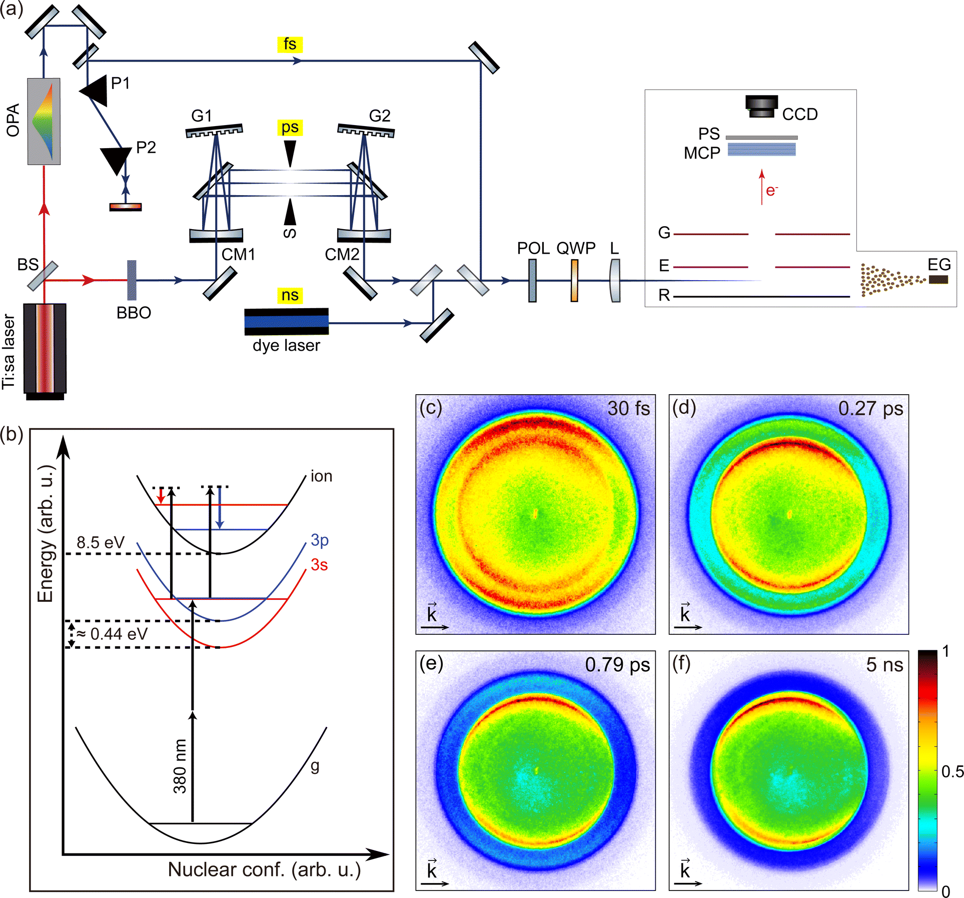 | ||
| Fig. 1 (a) Schematic diagram of the experimental setup. To generate femtosecond, picosecond, and nanosecond laser pulses centered at 380 nm, we used an optical parametric amplifier, the second harmonic output of a Ti:sapphire laser followed by a 4f pulse shaper, and a tunable dye laser. After controlling the polarization, the pulses were focused in the VMI spectrometer to interact with fenchone molecules supplied as effusive gas (EG). Photoelectrons from the interaction region were then amplified by the microchannel plates (MCP) and imaged on a phosphor screen. A CCD camera was used to accumulate the image on the phosphor screen. (b) 2 + 1 REMPI scheme of fenchone with 380 nm (≈ 3.26 eV) radiation. There are two intermediate resonances in the 2 + 1 REMPI scheme, namely 3s and 3p. The energy difference between the lowest edge of the two intermediate resonances is about 0.44 eV.28,31 As illustrated in the figure, the final ionization step does not change the vibrational levels according to the Δv = 0 propensity rule for parallel potential surfaces. (c–f) Raw photoelectron angular distributions (PADs) measured with S-(+)-fenchone by using LCP pulses with (c) 30 fs, (d) 0.27 ps, (e) 0.79 ps, and (f) 5 ns duration. The light propagation directions are left to right for all PADs and indicated with arrows on the PADs. Each PAD comprises two concentric circles. The inner circle corresponds to photoelectrons via the 3s intermediate, and the outer circle corresponds to the 3p intermediate. The influence of internal conversion is shown from PADs (c–f) as fading of the outer circle. | ||
Around 0.45 mJ of the available pulse energy was used by one of the two arms to pump an optical parametric amplifier (OPA) (TOPAS, Light Conversion). The central wavelength of the OPA light source was tuned to 380 nm with a bandwidth of about 7 nm (FWHM). The OPA delivered maximum pulse energy of 7 μJ at a repetition rate of 3 kHz. The dispersion of the pulse was managed by a pair of prisms (P1, P2). To obtain the shortest pulse at the interaction region, multiphoton ionization yield of xenon was maximized by tuning the prism compressor. A pulse duration of 30 fs was estimated from the spectrum using the time–bandwidth product and experimentally verified using a transient-grating frequency-resolved optical gating (TG FROG).
On the other arm, about 0.80 mJ of the pulse energy was used for pumping a 5 mm thick BBO crystal to generate narrow-band UV pulses around a central wavelength of 380 nm. The UV pulses were guided through a home-built 4f-optical pulse shaper. The first grating (G1) separates the optical frequencies spatially, then the cylindrical mirror (CM1) focuses the bundle of spatially separated frequency components in the Fourier plane. After passing through a mechanical slit (S) placed in the Fourier plane, the spatially separated frequency components are recombined by the second cylindrical mirror (CM2) and the second grating (G2). The 4f geometry of the pulse shaper was carefully adjusted to maintain zero dispersion of the pulse using a TG FROG. The pulse's bandwidth was narrowed by reducing the opening of the slit to vary the pulse duration. Several slit positions were selected for the experiment, and the spectral width of the pulse was measured at each slit position. For all slit positions, the central wavelength of the pulse, 380 nm, was kept constant. The setup could produce pulses from 0.27 ps to about 1 ps. The pulse durations were estimated by the time–bandwidth product assuming a flat phase and a Gaussian profile.
Nanosecond laser pulses were generated by a commercial dye laser (Cobra Stretch, Sirah Lasertechnik). Intracavity frequency-doubled output from a Q-switched Nd:YAG laser (Quanta-Ray INDI 30-20, Spectra-Physics) was used to pump the dye laser. For the PECD experiment, constantly circulating Styryl 8 in ethanol was used as a dye. The laser was set to 760 nm and then frequency-doubled. The final output pulses had a central wavelength of 380 nm with a pulse energy of 2.7 mJ at a repetition rate of 20 Hz. The pulse duration measured by a fast photodiode was 5 ns.
All laser pulses from the three different light sources were guided to a velocity-map imaging (VMI) spectrometer.46 A polarizer (POL) was used to ensure the initial polarization parallel to the table (P-polarized). An achromatic (B. Halle) quarter waveplate for a wide UV range generated circularly polarized light. The Stokes parameter |S3| for LCP and RCP pulses from all three light sources were above 99%. The pulses were then focused in the interaction region of the VMI spectrometer using a fused silica plano-convex lens of 250 mm focal length. The peak intensity of 9 × 10¹² W cm−2 of the shortest pulse (30 fs) leads to a Keldysh parameter γ ≈ 6, which is safely in the multiphoton regime. The photoelectrons from the interaction region were first amplified with microchannel plates (MCPs) in chevron configuration and imaged on a phosphor screen (PS). A CCD camera (Lumenera LW165m) was used to accumulate the photoelectron angular distribution (PAD) imaged on the phosphor screen. The polarization was switched between LCP and RCP after each accumulation of 500 frames with the CCD camera to compensate for long-term experimental drifts from the laser system or molecular gas pressure. The exposure time of the CCD camera was 132 ms, so a set of 500 frames corresponds to about 66 seconds. For each measurement, a total of 2500 frames was accumulated after five cycles of the polarization switching. For the dye laser measurement, 3500 frames were accumulated after seven polarization switching cycles to achieve a sufficient signal-to-noise ratio.
We used (S)-(+)-fenchone with 96% purity (Sigma-Aldrich) and (S)-(−)-camphor with 95% purity (Sigma-Aldrich) in the experiment. Fig. 1(b) shows the 2 + 1 resonance-enhanced multiphoton ionization (REMPI) scheme of fenchone with 380 nm (≈ 3.26 eV) radiation. As shown in Fig. 1(b), 380 nm radiation first excites two intermediate electronic states of fenchone, the 3s and the 3p, via a two-photon process. From the 3s and the 3p intermediates, the molecule can be ionized by single-photon absorption. The lowest edge of the 3s and the 3p states are respectively located at about 5.95 eV and about 6.39 eV, corresponding to a difference of about 0.44 eV.28,31 The adiabatic ionization potential of fenchone is 8.5 eV.26,31 Both the 3s and the 3p state are Rydberg states, so their potential energy surfaces are almost parallel to the continuum state's potential energy surface. Thus, the vibrational quantum number v is kept approximately constant in the ionization transitions from the 3s and the 3p intermediate states to the continuum state. Consequently, photoelectrons ionized via the 3s state correspond to higher v and therefore have lower kinetic energy than photoelectrons via the 3p state, as illustrated in Fig. 1(b).
Fig. 1(c–f) shows the raw PADs measured by using LCP pulses with four selected durations: 30 fs, 0.27 ps, 0.79 ps, and 5 ns. All pulse durations are given in terms of the FWHM of the temporal intensity profile. In a PAD, the distance from the image center to a specific position is proportional to the in-plane momentum of the electrons measured at that position. The energy calibration of PADs was done by using Xe atoms ionized by the third harmonic output (355 nm) of a Q-switched Nd:YAG laser as a reference. Here, the nanosecond laser source was chosen to exclude the ponderomotive shift in the calibration process. As shown in Fig. 1(c), each raw PAD has two concentric circles. The inner circle corresponds to the photoelectrons ionized via the 3s intermediate, and the outer one is via the 3p intermediate. The energy difference between the two circles corresponds to the energy difference between the two intermediates due to the Δv = 0 propensity rule in the last ionizing transition of the 2 + 1 REMPI. In addition, the relative intensity of the outer circle fades compared with the inner one as the pulse duration becomes longer. This behavior can be attributed to internal conversion dynamics of the molecule27,44 and will be discussed in the upcoming sections.
3 Experimental results
We measured PADs of fenchone in the gas phase by using laser pulses with various pulse durations from 30 fs to 5 ns. As mentioned above, the pulse duration was varied by adjusting the bandwidth of the laser pulses while keeping the central wavelength of 380 nm fixed. Consequently, the spectral width was not fixed over the experiment, and it was necessary to check for a uniform response to exclude sharp resonances over the spectral region. Thus, we first scanned the wavelength from 374 nm to 385 nm with a 1 nm step using a nanosecond dye laser. At each wavelength, photoelectrons were recorded with linear (LIN) polarization. The scanning range safely covers wavelengths within the FWHM of the broadest spectrum, 7 nm FWHM of the 30 fs pulse. Fig. 2(a) shows the resulting photoelectron energy spectra (PES) measured with LIN polarization. Each PES is individually normalized by setting the maximum value to 1. The prominent peak located between 0.5 eV and 0.9 eV in each curve is the photoelectron contribution ionized via the 3s intermediate state, and the broader distribution between 1.0 eV and 1.4 eV is the photoelectron contribution via the 3p. In every PES, there is another small peak located between 0.3 eV and 0.5 eV. The energy difference between the small peak and the 3s peak is about 0.37 eV, which matches with the energy of the CH stretch vibrations.47,48 Thus, we may attribute the small peak to Δv = 1 transition for a CH stretching vibrational mode in the final ionization step of the 2 + 1 REMPI via the 3s intermediate. This is an exception to the Δv = 0 propensity rule. All PES clearly show almost identical shapes except for a slight shift due to the photon energy difference. The identically shaped PES over several measurements with different wavelengths imply that the effect of sharp resonances in ionization pathways is negligible under our effusive beam conditions.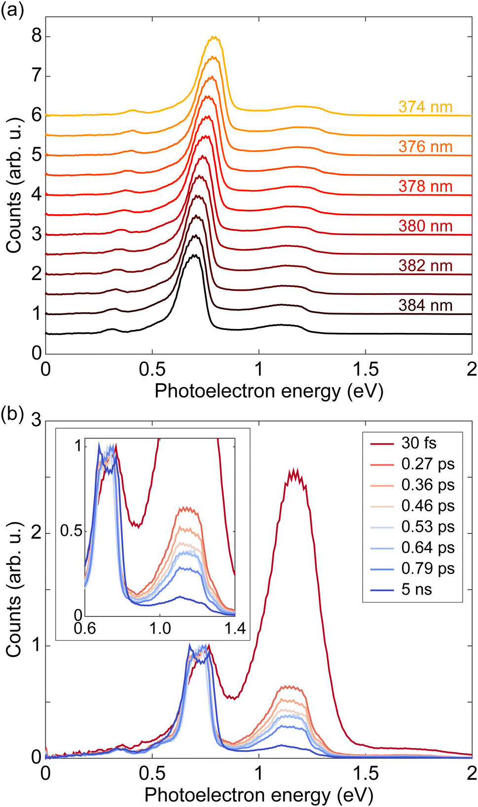 | ||
| Fig. 2 (a) Photoelectron energy spectra (PES) of (S)-(+)-fenchone from a wavelength scanning experiment with linearly polarized nanosecond pulses. The wavelength of the nanosecond dye laser was varied from 374 nm to 385 nm in 1 nm steps. Each PES is individually normalized by setting the maximum value to 1. There is no clear difference among the individually normalized results from different wavelengths except for the energy shift due to the change in photon energy. (b) PES of (S)-(+)-fenchone measured with circularly polarized pulses of various durations. The averages of PES from LCP and RCP measurements are shown. In each plot, the peak near 0.75 eV is ionized via the 3s intermediate state, and the peak near 1.2 eV is via the 3p intermediate state. The maximum of the 3s contribution is set to 1 to show the relative height of the 3p peaks. Note the decreasing 3p peak as the pulse duration becomes longer. A zoomed plot is provided in the inset. | ||
Fig. 2(b) shows the PES measured with various pulse durations using circularly polarized light centered at 380 nm, where the averages of PES from LCP and RCP measurements were used. The photoelectron contribution around 0.75 eV is ionized via 2 + 1 REMPI through the 3s intermediate state, and the photoelectron contribution near 1.2 eV is through the 3p intermediate state. As discussed above, the small peak around 0.4 eV may be attributed to Δv = 1 transition for a CH stretching vibrational mode in the ionization step via the 3s intermediate. The 3s peak in each curve is set to 1 for easier comparison of relative heights of the 3p peaks. A zoomed plot is provided in the inset of Fig. 2(b). We note that the PES measured by 30 fs pulse is shifted about 30 meV compared to the others. The shift is attributed to the beams slightly different divergence and focusing conditions in the VMI spectrometer. The relative height of the 3p peak to the 3s peak decreases as the pulse duration becomes longer. As noted before, this behavior can be attributed to internal conversion dynamics of the molecule with sub-picosecond time scales.27,44 The difference in the 3p peak shape between 30 fs PES and the others can be explained by the same reason. The 30 fs laser pulse is much faster than the time scale of the internal conversion. Therefore the 30 fs PES reflects almost only the absorption cross section. The PES measured by longer laser pulses undergo internal conversion, which reshapes the peak. Further analysis with a model system and estimation of lifetimes of these internal conversion processes will be given in the next section. All data were taken under the presence of a small oscillatory deflection of the electrons in the VMI on a 1 second time scale. The double-peaked structure of the 3s contribution in the 5 ns PES (also visible in the ns result in Fig. 3) is attributed to this oscillatory deflection becoming visible due to the higher spectral resolution and the lower repetition rate of the ns dye laser. The elongated central parts of the raw PADs in Fig. 1(c–f) are also attributed to this small imperfection.
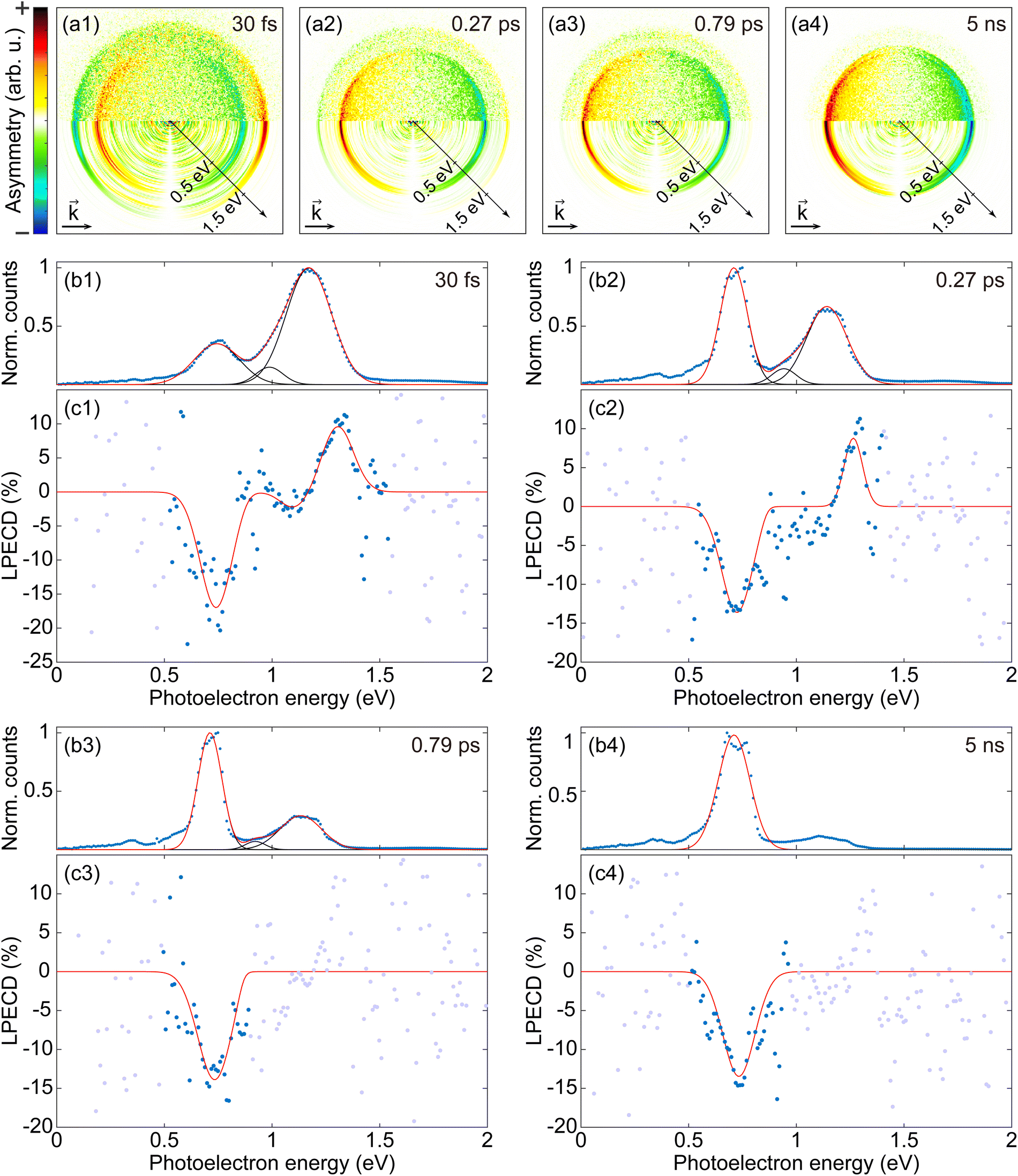 | ||
| Fig. 3 (a1–a4) Anti-symmetrized PECD images for (a1) 30 fs, (a2) 0.27 ps, (a3) 0.79 ps, and (a4) 5 ns measurements with S-(+)-fenchone. For each PECD image, the difference between an LCP PAD and an RCP PAD was calculated and then anti-symmetrized with respect to the vertical axis. The upper half of each image is obtained from raw PADs, and the lower half is obtained from Abel-inverted PADs. The inclined axis shows the calibrated energy scale. (b1–b4) Photoelectron energy spectra (PES) for (b1) 30 fs, (b2) 0.27 ps, (b3) 0.79 ps, and (b4) 5 ns measurements with S-(+)-fenchone. The averages of PES from LCP and RCP measurements are presented. The experimental data of PES is shown as blue dots in each plot and was fitted with (b1–b3) three Gaussians and (b4) a single Gaussian. Fitted Gaussians are plotted with black solid lines, and the total fitting result is plotted as a red solid line. (c1–c4) LPECD for (c1) 30 fs, (c2) 0.27 ps, (c3) 0.79 ps, and (c4) 5 ns measurements with S-(+)-fenchone. LPECD data were fitted using (c1) three Gaussians, (c2) two Gaussians, and (c3 and c4) a single Gaussian depending on the strength of the 3p part (see the main text for further details). Only the total fitting results are plotted as red solid lines. The experimental results are shown as blue dots in the region where the absolute value of the fitting result is greater than 0.1% and are shown as gray dots everywhere else. | ||
The raw PADs were processed through inverse Abel transform by using the pBasex algorithm.49 The original three-dimensional photoelectron distribution was retrieved under the assumption of axial symmetry with respect to a specific axis. For the circular polarization case, the axis of axial symmetry is parallel to the wave vector ![[k with combining right harpoon above (vector)]](https://www.rsc.org/images/entities/i_char_006b_20d1.gif) of the light, and the PECD appears along the direction of the symmetry axis. From the retrieved three-dimensional photoelectron distribution, a slice defined by a plane parallel to the detector and containing the symmetry axis is extracted and expanded into a series of Legendre polynomials. Legendre polynomials up to the sixth order were used to describe the PADs since the lowest order process, i.e., the three-photon ionization, is dominant in 2 + 1 REMPI in the weak-interaction regime.19,50 The symmetric and asymmetric parts of the photoelectron distribution are respectively expressed by even and odd orders of the Legendre polynomials. In this study, we only utilize the linear asymmetry in the photoelectron distribution, which is called linear photoelectron circular dichroism (LPECD),19 for the quantitative description of the chiral property. Using the coefficients ci for Legendre polynomial of order i, we first calculate
of the light, and the PECD appears along the direction of the symmetry axis. From the retrieved three-dimensional photoelectron distribution, a slice defined by a plane parallel to the detector and containing the symmetry axis is extracted and expanded into a series of Legendre polynomials. Legendre polynomials up to the sixth order were used to describe the PADs since the lowest order process, i.e., the three-photon ionization, is dominant in 2 + 1 REMPI in the weak-interaction regime.19,50 The symmetric and asymmetric parts of the photoelectron distribution are respectively expressed by even and odd orders of the Legendre polynomials. In this study, we only utilize the linear asymmetry in the photoelectron distribution, which is called linear photoelectron circular dichroism (LPECD),19 for the quantitative description of the chiral property. Using the coefficients ci for Legendre polynomial of order i, we first calculate
| ctotal0(E) = cLCP0(E) + cRCP0(E), |
| ctotali(E) = cLCPi(E) − cRCPi(E), i = 1,3,5,…, | (1) |
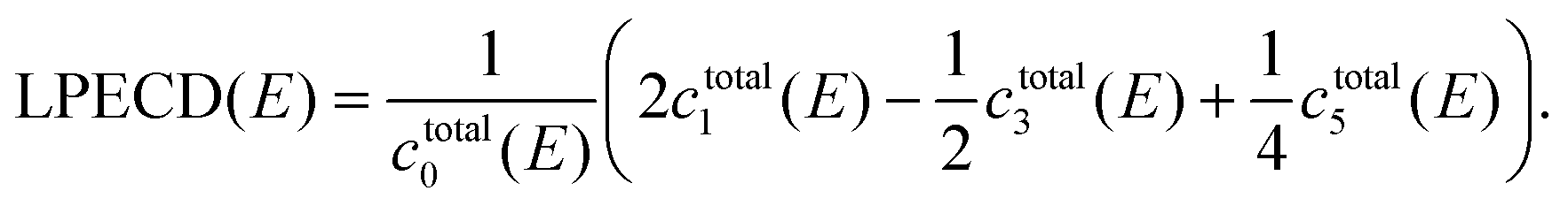 | (2) |
The LPECD is a normalized value with respect to the total photoelectron count ctotal0 as shown in eqn (2) and will be given in % throughout this article. Note that the Legendre coefficients ci and LPECD are functions of the photoelectron energy, E. We applied the same eqn (2) to calculate the LPECD value for each pulse duration using Legendre coefficients obtained from Abel inversion of the corresponding PAD.
Fig. 3 shows anti-symmetrized PECD images, PES, and LPECD for 30 fs, 0.27 ps, 0.79 ps, and 5 ns measurements. The top row (a1–a4) contains the anti-symmetrized PECD images. To obtain a PECD image, we first subtracted an RCP PAD from a corresponding LCP PAD and then anti-symmetrized the result with respect to the vertical axis. Note that the sign of the PECD, or the sign of the asymmetry, is opposite in an LCP PAD and an RCP PAD. The upper and lower half of the PECD images are respectively from raw PADs and Abel inverted PADs. The four sets of plots below the PECD images show the PES and LPECD as functions of photoelectron energy. Each set of plots consists of PES (b1–b4) and LPECD (c1–c4). As mentioned above, the peak near 0.75 eV corresponds to photoelectrons ionized via the 3s intermediate, and the peak near 1.2 eV corresponds to the 3p intermediate.
We fitted the PES with Gaussians to identify separable contributions. All PES except the 5 ns measurement were fitted with three Gaussians, one for the 3s contribution and the other two for the 3p contribution.26 The PES of the 5 ns measurement was fitted with only a single Gaussian for the 3s peak, as the 3p contribution was very small. In each PES plot, the experimental data are shown as blue dots, the fitted Gaussians are plotted as black solid lines, and the total sum of the Gaussians is plotted as a red solid line. The two 3p contributions of the PES might be attributed to electronic states reported in nanosecond laser experiments using jet-cooled fenchone28,31 and calculation results.31,34 However, we will not directly compare our results and the others since there is a significant difference in conditions between those results on jet-cooled molecules and our experiment using effusive molecular gas.
We employed a custom fitting method to reduce the effect of noise and to take account of possible asymmetries of peaks in the fitting process with LPECD: We first conducted two independent Gaussian fittings for PES and PES × LPECD, where the PES works as a window function for the LPECD. Then, the PES × LPECD fit function is divided by the PES fit function to obtain an effective fit function for LPECD. We did not set any assumptions for fitting parameters such as positions, widths, or heights of the Gaussians. The number of Gaussians for each fitting was decided via the strength and the shape of the 3p contribution. Two coupled fittings do not need to use the same number of Gaussians. For the results in Fig. 3(c1–c4), the PES×LPECD for 30 fs and 0.27 ps were respectively fitted with three Gaussians and two Gaussians. For both 0.79 ps and 5 ns, the PES× LPECD were fitted with a single Gaussian. The resulting effective fitting curves for each LPECD data is plotted as red solid lines in Fig. 3(c1–c4). The experimental result is shown as blue dots in the region where the value of the fit function is greater than 0.1% and shown as gray dots elsewhere. The Gaussian fitting results for PES×LPECD are provided in the ESI.†c1 and c2, the coefficients for the two lowest order Legendre polynomial terms, are also presented in the ESI.†
In order to extract a single LPECD value for the 3s peak of each pulse duration, we take the extreme value of the respective LPECD fit function. The results are presented in Table 1. The LPECD at the 3s peak seems more or less constant through all pulse durations, which is consistent with earlier observations.26–28
| Pulse duration | LPECD at 3s (%) |
|---|---|
| 30 fs | −17.0 ± 1.1 |
| 0.27 ps | −13.6 ± 0.6 |
| 0.36 ps | −14.0 ± 0.7 |
| 0.46 ps | −16.8 ± 0.7 |
| 0.53 ps | −13.4 ± 0.5 |
| 0.64 ps | −14.8 ± 0.6 |
| 0.79 ps | −13.6 ± 0.5 |
| 5 ns | −13.4 ± 0.5 |
The two distinct 3p LPECD peaks are labeled as 3pa and 3pb, where 3pa is the peak at lower photoelectron energy. The 3p photoelectron contributions are not separable into 3px, 3py, and 3pz substates in our measurement because of overlapping photoelectron contributions due to similar spacings of vibrational and electronic transitions.31 Therefore, we do not assign 3pa and 3pb to the 3p substates 3px, 3py, and 3pz. The photoelectron counts via the 3p intermediate decrease as the pulse duration becomes longer. As a result, both 3p peaks in LPECD emerge for the 30 fs result, but only the 3pb contribution can be seen in the 0.27 ps result. Moreover, the low counts of the 3p photoelectrons make it impossible to derive a statistically significant LPECD value for the 0.79 ps and 5 ns results. Thus, we provide the maximum 3p LPECD amplitude for prominent peaks only in Table 2. We cannot conclude about the 3p LPECD over the full range of pulse durations since the 3p LPECD values for long pulse durations cannot be obtained in the current study due to low photoelectron counts, although it appears to exist for long pulses. For the pulse durations with sufficient photoelectrons, the LPECD at the 3pb peak is constant within our error range.
| Pulse duration | LPECD at 3pa (%) | LPECD at 3pb (%) |
|---|---|---|
| 30 fs | −2.3 ± 1.3 | + 9.3 ± 2.8 |
| 0.27 ps | N/A | + 8.8 ± 2.2 |
| 0.36 ps | N/A | + 8.8 ± 3.8 |
For a deeper understanding of the dynamics, it is worth considering the differences among femtosecond, picosecond, and nanosecond pulse interactions with respect to the physical degrees of freedom we expect to be involved in these time scales. Pulse lengths of the order of few tens of femtoseconds are at the same time scale of the fastest nuclear dynamics. Thus, the fenchone molecule cannot undergo significant structural changes before the pulse has left. Since we expect the nuclear motion to be negligible, the interaction is described dominantly with light-driven transitions. Therefore, the ionized population measured with femtosecond pulses mainly reflects transition dipole moments among electronic states.
On the other hand, during the interaction with a nanosecond laser pulse, the system is affected by nuclear motion, for example, rotation, vibration, and intramolecular conversion. Interestingly, these processes do not seem to dramatically change the amplitude of PECD, as shown in Table 1. Note that we have excluded effects due to sharp resonances in the nanosecond measurements by the wavelength scanning described in Fig. 2(a). For molecules like fenchone, the nanosecond measurement does not depend on detailed resonances even in a region of a high density of vibrational states and gives a similar LPECD amplitude as the femtosecond measurement. In such a case, easier operation of nanosecond lasers than femtosecond lasers can be advantageous for PECD applications. In recent studies on supersonic molecular beams, the selectivity of REMPI excitation with the sensitivity of PECD was demonstrated by using a nanosecond laser tuned to the band origin of a low lying electronic state.28,43 These results open the door for chiral sensitivity measurements in mixtures and conformers.
Picosecond pulses can be regarded as an in-between choice and have the potential to show rich dynamics. For a specific experiment, one can choose an appropriate pulse duration or a spectral resolution between two extremes, femtosecond and nanosecond. A recent study using pulses with the pulse duration of 1.3 ps reported a significant variation of PECD of fenchone depending on different vibrational transitions.45 The predominance of the third Legendre polynomial to the PECD out of the 3s state, especially in the 6.46 eV excitation (two-photon excitation with 384 nm) result presented in the supplementary information,45 differed to results obtained with tunable femtosecond excitation26 as well as tunable nanosecond excitation28 on fenchone. In the same work,45 the Δv = 0 contribution of the PECD for the 3p state has the same sign with the Δv = 0 contribution of the PECD for the 3s state. Same-signed PECD for the 3s and the 3p was also reported in the experiment with 355 nm nanosecond laser.26 These results differ from the 30 fs, 0.27 ps, and 0.36 ps measurements in the current work, where the major contribution of the 3p PECD has the opposite sign to the 3s PECD. The PECD for the 3s and the 3p with opposite signs are consistent with tunable femtosecond excitation results.26 Thus, such different signs of the 3p PECD for varying pulse durations may be attributed to the ongoing molecular dynamics on longer time scales.
4 Model calculation
The results from the pulse duration scanning show a clear signature of internal conversion processes. As the pulse duration becomes longer, relative photoelectron counts via the 3s intermediate state increase compared to counts via the 3p. Such internal population conversion can be quantitatively studied with the PES data. For a deeper investigation, we constructed a model system to simulate the light–molecule interaction including internal conversions and simulated the dynamics by numerically solving the Lindblad master equation.Our model system of fenchone is shown in Fig. 4(a). The model system consists of a ground state, two intermediate states |3s〉 and |3p〉, and two ionic states |ion3s〉 and |ion3p〉. Each ionic state is coupled to the corresponding intermediate state. We place the excited |3s〉 and |3p〉 states at equal energies to match the absorbed photon energies. This placement at equal energies also accounts for the fact that different vibrational levels are accessed in each electronic state. Similarly, we represent the ionic continuum by a single state each for the 3s and the 3p pathway. We applied a fast population decay with a lifetime of 1 fs from each ionic continuum state to a respective dump state to mimic the decoherence due to escaping electrons. The transition dipole moment for each transition is written as μ(k)j,i where the superscript (k) is the number of photons involved and the subscripts i and j indicate the two states being coupled. To account for internal conversions, we introduce a cascading population decay |3p〉 → |3s〉 → |g〉 in the model system, illustrated with red curved arrows in Fig. 4 (a). Here, the specific decay pathway from |3s〉 is not revealed yet. We tested the model system to set a reasonable decay pathway from |3s〉. We found that directing the decay from |3s〉 to any dump state including |g〉 does not alter the overall dynamics under the assumption of weak interaction. We excluded dephasing (or T2 relaxation) in the intermediate states of our model system since the experiment was done in collision-free condition. The maximum pressure inside the VMI spectrometer chamber during the experiment was about 3 × 10⁻⁶ mbar, where the majority of the gas was fenchone (or camphor in case of camphor measurements).
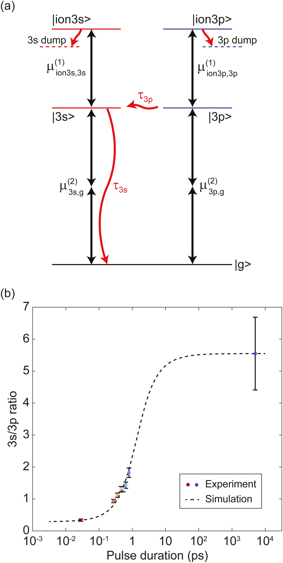 | ||
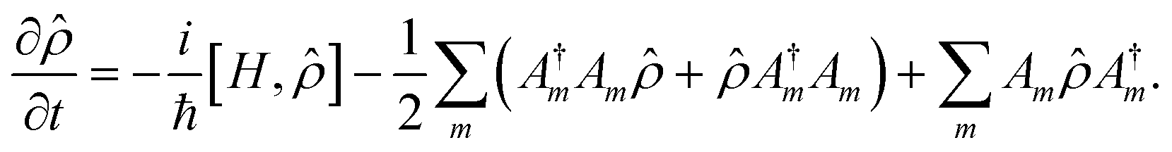
| Fig. 4 (a) A simplified model of fenchone. The model consists of a ground state |g〉, two intermediate states, |3s〉 and |3p〉, and two continuum states |ion3s〉 and |ion3p〉. Black arrows indicate transitions, and the number of arrows shows the number of involved photons. A cascading decay of |3p〉 → |3s〉 → |g〉 is illustrated as red curved arrows. A fast decay with a lifetime of 1 fs from each continuum state to a corresponding dump state is applied to mimic the decoherence due to escaping electrons. Dotted horizontal lines below continuum states represent dump states. (b) Experimental and simulation data of 3s/3p ion population ratios as functions of the pulse duration. Circles indicate the experimental data measured with S-(+)-fenchone using circularly polarized light, where the same color code as in Fig. 2(b) was employed to distinguish the data for different pulse durations. The dotted line shows the simulation data. By iteratively tuning the parameters of the model system in (a), our simulations were fitted to the experimental data. The larger error bar of the 5 ns point does not change the range of the lifetime estimation result given in Table 3. | ||
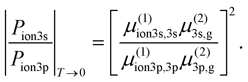
For the simulation of the dynamics including internal conversions and to estimate lifetimes of the intermediate states induced by these processes, we numerically solve the Lindblad master equation51
 | (3) |
![[small rho, Greek, circumflex]](https://www.rsc.org/images/entities/i_char_e0b7.gif) is the density matrix, H is the Hamiltonian, and Am are the Lindblad operators, which describe decay corresponding to each internal conversion channel m. We used square pulses for simplicity, and all interactions were carefully kept in the weak interaction regime. Using Gaussian pulses instead of square pulses does not alter the calculation result because the pulse spectrum is perfectly centered on the resonances in the calculation. We also do not expect off-resonant effects due to the wings of the spectrum of the square pulse playing a major role.
is the density matrix, H is the Hamiltonian, and Am are the Lindblad operators, which describe decay corresponding to each internal conversion channel m. We used square pulses for simplicity, and all interactions were carefully kept in the weak interaction regime. Using Gaussian pulses instead of square pulses does not alter the calculation result because the pulse spectrum is perfectly centered on the resonances in the calculation. We also do not expect off-resonant effects due to the wings of the spectrum of the square pulse playing a major role.
The four transition dipole moments and the two lifetimes of the internal conversions are unknown parameters in our model system. We determined these unknown parameters via an iterative process, such that the lifetimes of the internal conversions can be estimated. To this end, we used a fitting-like procedure: the parameters in the model system are iteratively tuned, and simulation data is calculated by numerically solving the Lindblad equation using the model system with trial parameter values at each iteration. The parameter values for the next iteration are set by comparing the simulation data with the experimental data. As the experimental data for this comparison, the 3s/3p ratio of total photoelectron counts for each pulse duration was calculated from the integrated 3s and 3p contributions of the experimentally obtained PES. For the simulation data, the ratio of |ion3s〉 population to |ion3p〉 population was calculated for each pulse duration point. The pulse durations sampled in our simulations are logarithmically spaced. Specifically, starting from the smallest value 100.5 fs (≈ 3.16 fs), the relation between the i-th and (i + 1)-th pulse duration point, Ti and Ti+1, is given by
| Ti+1 = 100.1Ti, | (4) |
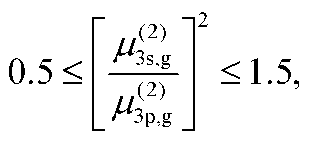
We now explain the details of the parameter determination process. We start from the short pulse limit of T → 0 where the dynamics is described only by the light-driven transitions. In this limit, the ratio of |ion3s〉 population to |ion3p〉 population is only defined by the transition dipole moments,
 | (5) |
Our shortest measurement (30 fs) approximates the T → 0 limit such that we can extract the value of the total ratio in eqn (5) from the experimental data. An independent estimation of the dipole moments for the two-photon resonant part and the one-photon ionization part in the 2 + 1 REMPI is not possible in our experiment. To overcome this, we used the computed transition strengths of fenchone from.31,34 A previous study31 provides calculated two-photon cross sections of fenchone, corresponding to the first two-photon resonance in the 2 + 1 REMPI, from a few different sources. In this previous study, the two-photon cross section of the 3p state is given in three components, and we calculated the rough total cross section of the 3p state by summing up all three. By adopting the computed values, the range of the two-photon dipole moments ratio for circular polarization is estimated as
 | (6) |
| Molecule | Fenchone | Camphor | ||||||
|---|---|---|---|---|---|---|---|---|
| 2-68-12 Polarization | CIRC | LIN | CIRC | LIN | ||||
| [μ(2)3s,g/μ(2)3p,g]2 | 0.5 | 1.5 | 0.2 | 0.3 | 2.0 | 5.0 | 0.30 | 0.65 |
| τ 3s (fs) | 400 | 320 | 470 | 410 | 360 | 330 | 380 | 340 |
| τ 3p (fs) | 110 | 80 | 120 | 90 | 170 | 140 | 230 | 150 |
In Table 3, we provide the minimum and the maximum values of [μ(2)3s,g/μ(2)3p,g]2 estimated from31,34 and corresponding estimations of lifetimes for the 3s and the 3p states. We investigated lifetimes for four cases: fenchone and camphor, with circularly or linearly polarized light. The estimated lifetimes given in Table 3 are from the best fits done with the two limits of [μ(2)3s,g/μ(2)3p,g]2. Thus, the lifetime results in Table 3 can be interpreted as ranges for our estimation of the lifetimes, e.g., 320 fs ≤ τ3s ≤ 400 fs and 80 fs ≤ τ3p ≤ 110 fs for fenchone interacting with circularly polarized light.
Fenchone and camphor have a similar electronic state structure since they are structural isomers: they have the same backbone structure and differ only in the placement of the peripheral methyl group. The adiabatic ionization potential of camphor is 8.66 eV52 which is slightly higher than 8.5 eV of fenchone. Compared to fenchone, camphor has about 112 meV higher band origin of the 3s state43 and about 140 meV higher band origin of the 3p state.53 Despite slightly higher energies of the states, 380 nm laser pulses still ionize camphor via 2 + 1 REMPI through the 3s and the 3p intermediate resonances. Therefore, the pulse duration scanning experiment with camphor was performed with 380 nm laser pulses as fenchone.
When determining [μ(2)3s,g/μ(2)3p,g]2 for camphor from computed transition strengths provided in ref. 34, we expect only one or two low-lying components of the 3p state among all three to be addressed by 380 nm laser pulses due to the band origin of the 3p state being about 140 meV higher compared to fenchone. Thus, we calculated [μ(2)3s,g/μ(2)3p,g]2 for two cases: only the lowest component excitation case and the two low-lying components excitation case. The results were used as rough ranges of [μ(2)3s,g/μ(2)3p,g]2.
The similarity of the estimated lifetimes for each molecule with two different light polarizations supports the validity of our lifetime estimation method. Comparing the lifetime results for fenchone and camphor with the same light polarization, lifetimes of the 3p state of camphor are over 50% longer than fenchone while lifetimes of the 3s state of camphor are slightly shorter. In the case of the 3s state, the slightly shorter lifetimes of the 3s state of camphor than fenchone qualitatively agree with pump–probe (201.3 nm LIN or CIRC pump, 400 nm CIRC probe) type 1 + 1' REMPI study.54
In the ESI,† we provide PES of fenchone measured with linear polarization and PES of camphor measured with linear and circular polarizations from the pulse duration scanning experiment. The results regarding the PECD of camphor are not presented due to insufficient photoelectron counts for a precise PECD analysis.
Fig. 4(b) shows an example of the best fit between the experimental data and the simulated data for fenchone with circularly polarized light. The experimental data of the 3s/3p total photoelectron counts ratio measured with circularly polarized light are plotted as circles, and the simulated data of the |ion3s〉/|ion3p〉 population ratio are plotted with a dotted line. The same color code as in Fig. 2(b) was applied to the experimental data to distinguish the data corresponding to different pulse durations. This specific simulation result was obtained with [μ(2)3s,g/μ(2)3p,g]2 = 0.5. We also provide the same plots as Fig. 4(b), for fenchone with linear polarization and for camphor with linear and circular polarizations in the ESI.†
In our simulations, the plateaus for the two extremal pulse duration, i.e., shorter than 10−2 ps and longer than 102 ps, show the asymptotic behaviors discussed above. The pulse duration regime shorter than 10−2 ps can be called a short pulse limit, where light-driven dynamics are dominant. Likewise, we can call the regime with a pulse duration longer than 102 ps the long pulse limit, where the influence of nuclear dynamics is apparent.
Relaxation dynamics of fenchone and camphor were previously studied by pump–probe methods.44,54 In the pump–probe study with fenchone,44 time-resolved PECD was measured with a pump–probe type 1 + 1′ REMPI scheme, comprising 201 nm, 80 fs, linearly polarized pump pulses, and 403 nm, 70 fs, circularly polarized probe pulses. This work estimated a time constant of 3.28 ps for the internal conversion from the 3s to a lower electronic state by analyzing exponential decays of PES. 201 nm pump radiation addresses vibrational states in the 3s intermediate state with about 0.36 eV lower energy than our 380 nm experiment. Such a significant energy difference between occupied vibrational states leads to a considerable difference in the density of states, which is closely related to the lifetime.55 In this regard, the shorter 3s state lifetime of around 400 fs in our estimation is not surprising. The pump–probe study with camphor54 used almost the same experimental method as for fenchone in ref. 44. The estimated time constant for the internal conversion from the 3s state of camphor was about 2.5 ps, and the lifetime depends on the light polarization. As we mentioned above, the slightly shorter lifetimes of the 3s state of camphor compared to fenchone at the same excitation energy qualitatively agree with the pump–probe study.
In the same pump–probe study with fenchone44, the time constant for decays of normalized Legendre coefficients b1 = c1/c0 and b3 = c3/c0 were measured as 3.25 ps and 1.4 ps for the 3s state. The 3.25 ps decay of the b1 coefficient was attributed to the population relaxation via internal conversion, and the 1.4 ps decay of the b3 coefficient was attributed to the rotational dephasing of the axis of the excited state. In addition, a transient decrease with a time constant of 400 fs was also observed only for b1, and intramolecular vibrational relaxation (IVR) was suggested as an explanation. Adopting all pictures from the pump–probe study into our work to explain the dynamics is inappropriate due to the large difference in the 3s lifetime. Moreover, our coherent measurement principle differs fundamentally from the pump–probe approach (see below).
Our study's remarkable constancy of the PECD over a wide range of pulse durations from femtoseconds to nanoseconds may be attributed to our higher excitation conditions. Here, we do not encounter sharp resonances (see Fig. 2(a)), and the observed lifetime of the internal conversion is much faster than the rotational dephasing. Such conditions are often met in higher excited states of molecules and may be a route for generalization to obtain PECD values independent of the pulse duration.
In this study, we adopted a new coherent pulse duration scanning method to observe the time-dependent dynamics of a molecular system. Here, we would like to compare our coherent pulse duration scanning method and the conventional pump–probe method as tools to study time-dependent dynamics. In the conventional pump–probe method, time-dependent dynamics are captured by sweeping the time delay between two pulses. At each time delay, the dynamics are recorded as a frame of a movie. The light-driven dynamics only occur during the very short impulse of the pump pulse, and only field-free evolution including relaxation happens after the pump pulse. The moments of the start and the probing of the dynamics are known in this method. Fitting methods based on classical considerations can evaluate such relaxation dynamics in most cases.
The pulse duration scan method measures the accumulation of the time evolution for different periods by varying the pulse duration. It might be comparable to adjusting the exposure time in photography. In this method, the system undergoes coherent interactions with the light field co-occurring with the decay processes, except for extremely short pulse cases where the decays can be neglected. This means that the moments of start and the probing of the dynamics are not known, which is fundamentally different from the pump–probe method. So it is important to include the coherent light--matter interaction in the description while the system is decaying simultaneously.
5 Conclusion
We investigated the dependence of the PECD of gas-phase fenchone on the duration of 380 nm laser pulses driving 2 + 1 REMPI. The pulse duration was varied from 30 fs to 5 ns in the experiment by utilizing three distinct light sources. The study found that the PECD measured via the 3s intermediate is robust over five orders of magnitude of the pulse duration despite ongoing molecular dynamics. The findings may be more general in cases of excitation of molecules in higher excited states. We also estimated time constants of the cascading internal conversion |3p〉 → |3s〉 → |g〉 using a simplified model system. For instance, the results for fenchone with circularly polarized light are in ranges of 320 fs ≤ τ3s ≤ 400 fs and 80 fs ≤ τ3p ≤ 110 fs. This study's coherent pulse duration scanning method may stimulate a so far unexplored approach to unravel time-dependent intramolecular dynamics.Author contributions
H. L., S. T. R., and S. V. conducted the experiment; H. L. and S. T. R. analyzed the data; N. L. developed data analysis method; H. L. and D. M. R. developed theoretical model and performed simulation; T. R. helped maintenance of the experimental setup; S. D. and J. G. assisted data acquisition; H. B., A. S., and T. B. contributed on developing the idea; H. L. wrote the manuscript with contributions from S. V., H. B., D. M. R., A. S., and T. B.; H. B. and A. S. helped supervision; D. M. R. helped supervision regarding theory and numerics; T. B. supervised the project; all authors commented on the manuscript.Conflicts of interest
There are no conflicts to declare.Acknowledgements
Funding by the Deutsche Forschungsgemeinschaft (DFG, German Research Foundation) – Projektnummer 328961117 – SFB 1319 ELCH is gratefully acknowledged. We thank A. Kastner and T. Ring for experimental support in an early stage of the experiment.Notes and references
-
Chiral Recognition in the Gas Phase, ed. A. Zehnacker, CRC Press, Boca Raton FL USA, 1st edn, 2010 Search PubMed
.
- S. R. Domingos, C. Pérez and M. Schnell, Annu. Rev. Phys. Chem., 2018, 69, 499–519 CrossRef CAS PubMed
- U. Boesl and A. Kartouzian, Annu. Rev. Anal. Chem., 2016, 9, 343–364 CrossRef CAS PubMed
- L. Nahon, G. A. Garcia and I. Powis, J. Electron Spectrosc. Relat. Phenom., 2015, 204, 322–334 CrossRef CAS
- M. Pitzer, R. Berger, J. Stohner, R. Dörner and M. Schöffler, Chimia, 2018, 72, 384–388 CrossRef CAS PubMed
- C. Logé, A. Bornschlegl and U. Boesl, Int. J. Mass Spectrom., 2009, 281, 134–139 CrossRef
- C. Logé and U. Boesl, Chem. Phys. Chem., 2011, 12, 1940–1947 CrossRef PubMed
- T. Ring, C. Witte, S. Vasudevan, S. Das, S. T. Ranecky, H. Lee, N. Ladda, A. Senftleben, H. Braun and T. Baumert, Rev. Sci. Instrum., 2021, 92, 033001 CrossRef CAS PubMed
- K. Fehre, N. M. Novikovskiy, S. Grundmann, G. Kastirke, S. Eckart, F. Trinter, J. Rist, A. Hartung, D. Trabert, C. Janke, G. Nalin, M. Pitzer, S. Zeller, F. Wiegandt, M. Weller, M. Kircher, M. Hofmann, L. P. H. Schmidt, A. Knie, A. Hans, L. B. Ltaief, A. Ehresmann, R. Berger, H. Fukuzawa, K. Ueda, H. Schmidt-Böcking, J. B. Williams, T. Jahnke, R. Dörner, M. S. Schöffler and P. V. Demekhin, Phys. Rev. Lett., 2021, 127, 103201 CrossRef CAS PubMed
- C. Pérez, A. L. Steber, A. Krin and M. Schnell, J. Phys. Chem. Lett., 2018, 9, 4539–4543 CrossRef PubMed
- K. Fehre, S. Eckart, M. Kunitski, C. Janke, D. Trabert, M. Hofmann, J. Rist, M. Weller, A. Hartung, L. P. H. Schmidt, T. Jahnke, H. Braun, T. Baumert, J. Stohner, P. V. Demekhin, M. S. Schöffler and R. Dörner, Phys. Rev. Lett., 2021, 126, 083201 CrossRef CAS PubMed
- A. A. Milner, J. A. M. Fordyce, I. MacPhail-Bartley, W. Wasserman, V. Milner, I. Tutunnikov and I. S. Averbukh, Phys. Rev. Lett., 2019, 122, 223201 CrossRef CAS PubMed
- D. Baykusheva and H. J. Wörner, Phys. Rev. X, 2018, 8, 031060 CAS
- B. Ritchie, Phys. Rev. A: At., Mol., Opt. Phys., 1976, 13, 1411–1415 CrossRef
- N. Böwering, T. Lischke, B. Schmidtke, N. Müller, T. Khalil and U. Heinzmann, Phys. Rev. Lett., 2001, 86, 1187 CrossRef PubMed
- G. A. Garcia, L. Nahon, M. Lebech, J. C. Houver, D. Dowek and I. Powis, J. Chem. Phys., 2003, 119, 8781–8784 CrossRef CAS
- C. Lux, M. Wollenhaupt, T. Bolze, Q. Liang, J. Köhler, C. Sarpe and T. Baumert, Angew. Chem., Int. Ed., 2012, 51, 5001–5005 CrossRef CAS PubMed
- C. S. Lehmann, N. Bhargava Ram, I. Powis and M. H. M. Janssen, J. Chem. Phys., 2013, 139, 234307 CrossRef PubMed
- C. Lux, M. Wollenhaupt, C. Sarpe and T. Baumert, Chem. Phys. Chem., 2015, 16, 115–137 CrossRef CAS PubMed
- C. Lux, A. Senftleben, C. Sarpe, M. Wollenhaupt and T. Baumert, J. Phys. B: At., Mol. Opt. Phys., 2016, 49, 02LT01 CrossRef
- S. Beaulieu, A. Ferré, R. Géneaux, R. Canonge, D. Descamps, B. Fabre, N. Fedorov, F. Légaré, S. Petit, T. Ruchon, V. Blanchet, Y. Mairesse and B. Pons, New J. Phys., 2016, 18, 102002 CrossRef
- S. Beauvarlet, E. Bloch, D. Rajak, D. Descamps, B. Fabre, S. Petit, B. Pons, Y. Mairesse and V. Blanchet, Phys. Chem. Chem. Phys., 2022, 24, 6415–6427 RSC
- S. Beaulieu, A. Comby, D. Descamps, B. Fabre, G. A. Garcia, R. Géneaux, A. G. Harvey, F. Légaré, Z. Mašín, L. Nahon, A. F. Ordonez, S. Petit, B. Pons, Y. Mairesse, O. Smirnova and V. Blanchet, Nat. Phys., 2018, 14, 484–489 Search PubMed
- A. Kastner, C. Lux, T. Ring, S. Züllighoven, C. Sarpe, A. Senftleben and T. Baumert, Chem. Phys. Chem., 2016, 17, 1119–1122 CrossRef CAS PubMed
- J. Miles, D. Fernandes, A. Young, C. Bond, S. W. Crane, O. Ghafur, D. Townsend, J. Sá and J. B. Greenwood, Anal. Chim. Acta, 2017, 984, 134–139 CrossRef CAS PubMed
- A. Kastner, T. Ring, B. C. Krüger, G. B. Park, T. Schäfer, A. Senftleben and T. Baumert, J. Chem. Phys., 2017, 147, 013926 CrossRef PubMed
- A. Kastner, T. Ring, H. Braun, A. Senftleben and T. Baumert, Chem. Phys. Chem., 2019, 20, 1416–1419 CAS
- A. Kastner, G. Koumarianou, P. Glodic, P. C. Samartzis, N. Ladda, S. T. Ranecky, T. Ring, S. Vasudevan, C. Witte, H. Braun, H.-G. Lee, A. Senftleben, R. Berger, G. B. Park, T. Schäfer and T. Baumert, Phys. Chem. Chem. Phys., 2020, 22, 7404–7411 RSC
- M. M. Rafiee Fanood, M. H. M. Janssen and I. Powis, J. Chem. Phys., 2016, 145, 124320 CrossRef PubMed
- H. Ganjitabar, D. P. Singh, R. Chapman, A. Gardner, R. S. Minns, I. Powis, K. L. Reid and A. Vredenborg, Mol. Phys., 2020, 119, e1808907 CrossRef
- D. P. Singh, N. de Oliveira, G. A. Garcia, A. Vredenborg and I. Powis, Chem. Phys. Chem., 2020, 21, 2468–2483 CrossRef CAS PubMed
- M. N. Pohl, S. Malerz, F. Trinter, C. Lee, C. Kolbeck, I. Wilkinson, S. Thürmer, D. M. Neumark, L. Nahon, I. Powis, G. Meijer, B. Winter and U. Hergenhahn, Phys. Chem. Chem. Phys., 2022, 24, 8081–8092 RSC
- P. Krüger and K.-M. Weitzel, Angew. Chem., Int. Ed., 2021, 60, 17861–17865 CrossRef PubMed
- R. E. Goetz, T. A. Isaev, B. Nikoobakht, R. Berger and C. P. Koch, J. Chem. Phys., 2017, 146, 024306 CrossRef CAS PubMed
- A. N. Artemyev, A. D. Müller, D. Hochstuhl and P. V. Demekhin, J. Chem. Phys., 2015, 142, 244105 CrossRef PubMed
- A. D. Müller, A. N. Artemyev and P. V. Demekhin, J. Chem. Phys., 2018, 148, 214307 CrossRef PubMed
- A. D. Müller, E. Kutscher, A. N. Artemyev and P. V. Demekhin, J. Chem. Phys., 2020, 152, 044302 CrossRef PubMed
- A. F. Ordonez and O. Smirnova, Phys. Rev. A, 2018, 98, 063428 CrossRef CAS
- A. F. Ordonez and O. Smirnova, Phys. Rev. A, 2019, 99, 043416 CrossRef CAS
- A. F. Ordonez and O. Smirnova, Phys. Rev. A, 2019, 99, 043417 CrossRef CAS
- A. N. Artemyev, E. Kutscher and P. V. Demekhin, J. Chem. Phys., 2022, 156, 031101 CrossRef CAS PubMed
- C. Sparling, A. Ruget, N. Kotsina, J. Leach and D. Townsend, Chem. Phys. Chem., 2021, 22, 76–82 CrossRef CAS PubMed
- S. T. Ranecky, G. B. Park, P. C. Samartzis, I. C. Giannakidis, D. Schwarzer, A. Senftleben, T. Baumert and T. Schäfer, Phys. Chem. Chem. Phys., 2022, 24, 2758–2761 RSC
- A. Comby, S. Beaulieu, M. Boggio-Pasqua, D. Descamps, F. Legare, L. Nahon, S. Petit, B. Pons, B. Fabre, Y. Mairesse and V. Blanchet, J. Phys. Chem. Lett., 2016, 7, 4514–4519 CrossRef CAS PubMed
- D. P. Singh, J. O. F. Thompson, K. L. Reid and I. Powis, J. Phys. Chem. Lett., 2021, 12, 11438–11443 CrossRef CAS PubMed
- A. T. J. B. Eppink and D. H. Parker, Rev. Sci. Instrum., 1997, 68, 3477–3484 CrossRef CAS
-
NIST Chemistry WebBook, NIST Standard Reference Database Number 69, ed. P. J. Linstrom and W. G. Mallard, National Institute of Standards and Technology, Gaithersburg MD, 2022, p. 20899 Search PubMed
-
P. Larkin, Infrared and raman spectroscopy: Principles and spectral interpretation, Elsevier, Amsterdam [Netherlands] and Boston, 2011 Search PubMed
- G. A. Garcia, L. Nahon and I. Powis, Rev. Sci. Instrum., 2004, 75, 4989–4996 CrossRef CAS
- C. N. Yang, Phys. Rev., 1948, 74, 764–772 CrossRef CAS
-
H.-P. Breuer and F. Petruccione, The theory of open quantum systems, Oxford Univ. Press, Oxford, Reprint edn, 2010 Search PubMed
- L. Nahon, G. A. Garcia, H. Soldi-Lose, S. Daly and I. Powis, Phys. Rev. A: At., Mol., Opt. Phys., 2010, 82, 032514 CrossRef
- F. Pulm, J. Schramm, J. Hormes, S. Grimme and S. D. Peyerimhoff, Chem. Phys., 1997, 224, 143–155 CrossRef CAS
- V. Blanchet, D. Descamps, S. Petit, Y. Mairesse, B. Pons and B. Fabre, Phys Chem Chem Phys., 2021, 23, 25612–25628 RSC
- T. Baumert, J. L. Herek and A. H. Zewail, J. Chem. Phys., 1993, 99, 4430–4440 CrossRef CAS
Footnote |
| † Electronic supplementary information (ESI) available. See DOI: https://doi.org/10.1039/d2cp03202c |
| This journal is © the Owner Societies 2022 |