Optimization framework for redox flow battery electrodes with improved microstructural characteristics

Abstract

This research aims to advance the field of vanadium redox flow batteries (VRFBs) by introducing a pioneering approach to optimize the microstructural characteristics of carbon cloth electrodes. Addressing the traditional challenge of developing high-performance electrode materials for VRFBs, this study employs a robust, generalizable, and cost-effective data-driven modeling and optimization framework. A novel sampling strategy using low-discrepancy Latin Hypercube and quasi-Monte Carlo methods generates a small-scale, high-fidelity dataset with essential space-filling qualities for training supervised machine learning models. This study goes beyond conventional methods by constructing two surrogate models: a random forest regressor and a gradient boosting regressor as objective functions for optimization. The integration of a non-dominated sorting genetic algorithm II (NSGA-II) for multi-objective optimization facilitates exhaustive exploration of the surrogate models, leading to the identification of electrode designs that yield enhanced energy efficiencies (EEs) under specific operating conditions. The application of NSGA-II in exploring surrogate models not only facilitates the discovery of realistic design combinations but also adeptly manages trade-offs between features. The mean pore diameter was reduced compared to the tested carbon cloth electrodes while maintaining a similar permeability value based on the results obtained using the developed algorithms. Based on this suggestion, a new type of carbon cloth electrode has been fabricated by introducing a carbonaceous binder into the woven fabric to make carbon cloths with more complex pore structures and reduced mean pore diameter. The new electrode demonstrates 24% and 66% reduction in average ohmic and mass transport resistances, respectively, validating the machine-learning recommendations. This research highlights the critical role of improved electrical conductivity and porosity in carbon materials, showing their direct correlation with increased EE. Overall, this study represents a significant step forward in developing more efficient and practical VRFBs, offering a valuable contribution to the renewable energy storage landscape.

---

1. Introduction

The current climate crisis has underscored the need for net-zero carbon emission policies, both in the United States and globally.¹ Following the United States’ re-entry into the Paris Agreement in 2021, a long-term strategy was established with the goal of reaching net-zero carbon emissions by 2050. A critical milestone of this strategy is the 50–52% reduction in greenhouse gas emissions by 2030, necessitating a shift away from fossil fuels across all economic sectors. This decarbonization milestone is expected to increase electricity demand by approximately 50% over the next 10 years.¹ The surge in electricity demand poses significant challenges due to (i) the complex and failure-prone architecture of current electrical grid systems and (ii) the fact that 60% of electrical energy is currently supplied by fossil fuels.^2–4 Therefore, addressing the rise in electricity demand is crucial for sustaining the energy requirements necessary for a transition to a cleaner future.⁵

In recent decades, renewable energy technologies such as wind and solar, have experienced significant market growth. Despite their increasing popularity, these low-carbon alternatives are sometimes considered unreliable for long-duration demands due to their intermittent nature.⁶ To address this issue and balance the energy supply and demand, cost-effective, large-scale energy storage capabilities are essential.^7,8

Among the potential candidates for large-scale stationary energy storage are lead–acid batteries, lithium-ion (Li-ion) batteries, pumped storage hydropower (PSH), compressed air energy storage (CAES), and redox flow batteries (RFB).⁹ Li-ion batteries, predominant in consumer electronics and electric vehicles (EVs), face obstacles in grid-scale energy storage implementation due to their limited natural abundance and high cost for long-duration solutions.^9–12 PHS and CAES, while effective, require specific conditions for safe operation and are geographically restricted due to the necessity for suitable topography. These challenges are extensively discussed in review studies.^4,6,8,13,14

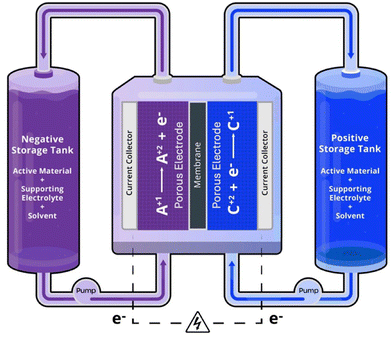
The search for a highly efficient, reliable, large-scale, and modular energy storage system continues to be a focus of active research.¹⁵ Among various options, RFB technology has received considerable attention due to its scalability, efficiency, safety, and cost-effectiveness for long-duration storage.^16–19 VRFBs, where vanadium serves as the electroactive species that is dissolved in the electrolyte, are the most common RFB technology.²⁰ In RFBs, energy is attributed to the charged active species in the electrolytes; enabling decoupled power generation and energy storage – a key feature that underscores the promise of RFBs for grid-scale and long-duration energy storage.^18,21–23Fig. 1 illustrates the structure of a RFB setup, with the negative and positive half-cells are separated by an ion exchange membrane. The negative and positive electrodes, critical for facilitating electrochemical reactions and providing pathways for reactant/product transport, are shown.

Fig. 1 Schematic of a RFB – A and C represent the redox active materials in the negative and positive electrolytes, respectively. In a VRFB, the negative electrolyte has V²⁺/V³⁺ and the positive electrolyte has V⁴⁺/V⁵⁺ redox couples.

The major obstacle to the global implementation of VRFB technology is their high capital cost. Large-scale commercialization will remain unrealistic until the capital costs of VRFBs are reduced to meet the DOE's cost target of $100 per kW h.²⁴ Performance improvement, achieved by increasing power-density and reducing resistances, will lead to reduced system costs.^25,26 Enhancing power density involves research focused on performance diagnostics at the cell level and improving the functionality and efficiency of components.²⁷

The porous electrode plays a crucial role in key functions such as facilitating ion/charge transfer, providing reaction sites for electrochemical reactions, and distributing liquid electrolytes.^27–32 Positioned adjacent to current collectors, which typically have flow channels machined within, porous electrodes benefit from interdigitated flow channel designs that increase average velocity and enhance overall battery performance.^30,33,34 Amongst other cell-level components, porous carbon electrodes are yet to be fully customized specifically for RFB applications. Operating conditions such as current density, flow rate, temperature, and electrolyte composition heavily impact the functionality of the porous carbon electrode, meaning that there is no singular optimal electrode design; performance will vary significantly based on operating conditions. Research aimed at improving the morphology of porous carbon electrodes has focused on maximizing active surface area for redox reactions and enhancing pathways for effective electrolyte transport.^35–38

Recent studies have made significant contributions to understanding and improving electrode materials for VRFBs. For example, Zhou et al. explored highly permeable carbon cloth electrode materials for VRFBs, investigating the activation of carbon cloth with KOH to increase active surface area. This study demonstrated that woven carbon fiber arrangements enhance mass transport, with the KOH-activated carbon-cloth electrode achieving notable performance metrics: at a current density of 400 mA cm⁻², the VRFB displayed an energy efficiency of 80.1% and electrolyte utilization of 74.6%.³⁹ The improved performance seen in the VRFB with carbon cloth electrodes could be attributed to the low tortuosity, low pressure drops, and high ionic conductivity associated with the larger pore sizes.³⁹ Furthermore, Forner-Cuenca et al. conducted a thorough investigation of three commonly used carbon fiber-based electrode materials: carbon paper, carbon felt, and carbon cloth to understand the influence of carbon cloth microstructure on electrode performance through microscopic, analytical, and electrochemical methods under fixed operating conditions.⁴⁰ The research presented by Nourani et al. aligns with the conclusions made by Tenny et al., indicating that while all three carbon fiber materials have benefits and drawbacks, the structured, ordered arrangement of fibers in carbon cloth can be strategically modified or tuned.^41,42 Thus, it can be concluded that significant performance improvements can be achieved with fabric, carbon cloth electrodes due to their tunable microstructure and ability to create structured woven patterns.

Previous investigations have identified key microstructural characteristics that affect the functionality of porous carbon electrodes, such as porosity, fiber diameter, and active surface area.^27,43–45 However, the expenses associated with laboratory-scale testing are often impractical, leading most studies to include limited experimental results supplemented with synthetic data that is collected numerically or computationally via zero-to-three-dimensional modeling.^46–51 To augment sparse datasets, it has become customary to incorporate machine learning (ML) techniques to aid the data generation process. Wan et al., for instance, proposed a coupled machine learning and genetic algorithm approach to design porous electrodes for RFBs.⁵² By created a dataset of 2275 fibrous electrode structures using a stochastic reconstruction method to generate three-dimensional fibrous structures, and then applying the Lattice Boltzmann method and a morphological algorithm to calculate specific surface area and hydraulic permeability, the authors were able to use a genetic algorithm to screen and pinpoint morphological traits of 700 porous electrode candidates. Results showed that fiber diameter (d_f) and porosity (ε) are impactful structural properties, and that tuning these properties can increase hydraulic permeability and specific surface area by 50% and 80%, respectively, thus improving overall energy efficiency.⁵²

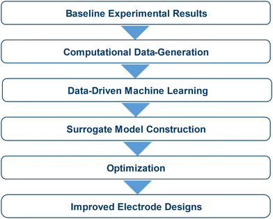
As an emerging technology, much remains to be discovered about the electrochemical and physical properties of carbon cloth electrodes in VRFBs. This research highlights that improved electrode designs can be uncovered using interpretable ML methods to develop cost-effective and generalizable surrogate models. While the methodology is focused on vanadium chemistries, it can be extended to various flow battery chemistries, offering a versatile approach for researchers to apply to their specific conditions. This modeling and optimization framework will reveal improved electrode designs that can be mapped back to the physical domain, providing insight and quantifiable metrics that can be associated with specific and ordered fiber arrangements. The sequential steps taken to reach improved electrode properties within the modeling and optimization framework are outlined below:

• Baseline experimental microstructure characterization and performance results are obtained to gain a physical understanding of structure–property–performance linkages.

• Experimental results are used to enhance a 2D COMSOL Multiphysics® model of a VRFB. This model is used for data-generation.

• A high-fidelity sampling plan is designed with Latin Hypercube Sampling (LHS) using Quasi-Monte-Carlo methods. This modified LHS strategy uses low-discrepancy methods to uniformly distribute an arbitrarily small number of samples (n < 500) throughout the design domain. The space-filling quality of this plan is not compromised when implemented in high-dimensions.

• The data-generation process consists of acquiring responses for each sample (electrode design) in the modified LHS plan. The charge–discharge curves produced by the computational model are used to calculate the response information for each sample. Three response values are calculated: energy efficiency (EE), coulombic efficiency (CE), and voltage efficiency (VE). This computational data-generation step will result in training data to support the data-driven modeling.

• Supervised regression techniques are utilized to produce an ML-based surrogate model with high prediction accuracy. Multi-output gradient boosting regression models and multi-output random forest regression models result in the lowest prediction error. A multi-output regressor is crucial to develop a surrogate model that accurately maps the relationships between the input design variables and the three target values.

• Multi-objective optimization then explores the surrogate model to obtain a Pareto set of design solutions. A nondominated genetic sorting algorithm-II (NGSA-II) is an elite multi-objective optimization algorithm that will maximize the efficiency targets while managing tradeoffs between the three target efficiencies to produce a set of the most advantageous designs.

• Combining the well-defined design constraints, accurate ML based surrogate modeling process, and optimization with NSGA-II increases likelihood that one of the designs in the Pareto set will be manufacturable.

The overall structure of this study and the elemental steps taken to develop this framework are highlighted in Fig. 2.

Fig. 2 Workflow diagram illustrating the multi-stage framework development process.

2. Methodology

2.1 Experimental Benchmarking

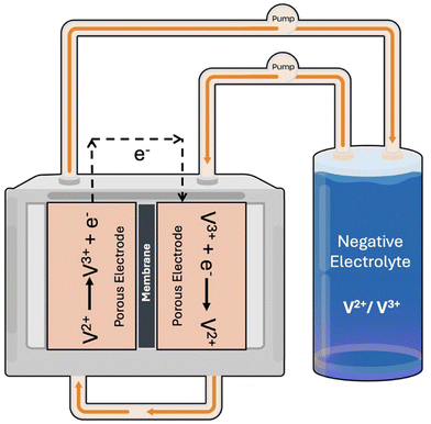
Carbon cloth electrode samples with different woven patterns, provided by AvCarb Material Solutions in Lowell, MA, are tested in the laboratory. The following AvCarb carbon fabric samples are assessed: 1698, 1615, 7497, 1185, 1698, 1070.⁵³ The experimental setup is a single tank symmetric cell, where the negative electrolyte is circulated through both sides of an interdigitated flow field at 80 mL min⁻¹. The cell is assembled with zero gap architecture and a 5-cm² geometrical area. Nafion 212 is selected as the membrane which separates two layers of carbon cloth electrodes that are placed on either side of the cell. With the use of a Bio-Logic SP-240 potentiostat coupled with EC-Lab software, electrochemical impedance spectroscopy (EIS) is performed on a symmetric, single tank VRFB cell with electrolyte composition of 1.5 M vanadium (V²⁺/V³⁺) and 3 M sulfuric acid at 50% SOC. To mitigate potential oxidation of V²⁺, nitrogen gas is flowed constantly within the electrolyte storage tank. A ±200 mV overpotential is applied for 24 hours with EIS experiments carried out every 4 hours.⁴⁴ With the use of data from EIS, the resistances associated with the electrodes can be quantified and used as a benchmark for electrode performance. Fig. 3 depicts the experimental test setup. The insights gained from the baseline experimental results are directly or indirectly mapped to global parameters in the computational model to support and enhance the data-generation process.

Fig. 3 Schematic of the experimental setup: a single tank symmetric VRFB cell.

2.2 COMSOL multiphysics® model for computational data-generation

Due to the intensive time and resource demands of testing critical structural properties of porous carbon electrodes, an experimentally validated computational model supports the data-driven modeling approach. This computational model, detailed in previous studies,^28,29,54 was validated experimentally, and the transient, isothermal computation model in COMSOL Multiphysics® simulation software incorporates vanadium crossover and water transport through the membrane, along with all the corresponding losses. The baseline experimental microstructure characterization and performance data enhance the computational model and guide the initial feature selection process.

2.3 Feature selection process

Identifying microstructural characteristics that enhance the performance of porous carbon electrodes requires extensive laboratory-scale testing. However, due to time and resource constraints, experimental data may be limited, thus serving as benchmark results that guide the incorporation of a computational model for data generation. These outcomes also play a crucial role in the feature selection process, where an initial set of design parameters or features (microstructural traits of porous carbon cloth media) that influence electrode functionality is identified. The primary stages of this process are illustrated in Fig. 4.

Fig. 4 Schematic outlining the four primary stages in the feature selection process.

2.3.1 Stage 1: selecting an initial set of electrode features. Selecting the initial set of electrode features is heavily influenced by the experimental observations. The initial set of features will be further analyzed in Stage 2. The following measurements were obtained from the laboratory experiments and used to influence the feature selection process:

i. Pore size distribution, tortuosity, specific surface area, and porosity measurements.

ii. Electrolyte flow resistance measurements.

iii. Charge transport resistance measurements.

iv. Mechanical properties and surface feature characterization is achieved.

v. Flow cell performance is evaluated by collecting polarization curves, charge/discharge curves for cycling analysis to determine area specific resistance (ASR) and energy efficiency (EE).

The initial features are displayed in Table 1 along with their units in the computational model. Each feature has a lower bound, upper bound, and recommended step size that were defined based on the baseline experimental setup and physical limitations of the materials or operating conditions that are being used in the lab. The full set of features that were initially considered and their subsequent ranges are displayed in the table below.

Table 1 Initial set of selected electrode features that are defined as global parameters in the computational model

Parameter description	Units	Lower bound	Upper bound	Step size
Porosity	%	0.7	0.97	0.03
Electrical conductivity of the electrode	S m^−1	66.7	66.7	—
Current density	A m^−2	1000	1500	100
Permeability of the electrode	m^2	1.0 × 10^−10	5.0 × 10^−10	0.01 × 10^−10
Mean pore diameter	m	1.0 × 10^−4	1.2 × 10^−4	0.001 × 10^−4
Average fiber diameter	m	1.0 × 10^−5	2.0 × 10^−5	1.0 × 10^−7
Reaction rate constant for reaction (1)	m s^−1	1.0 × 10^−8	9.0 × 10^−8	0.1 × 10^−8
Reaction rate constant for reaction (2)	m s^−1	1.0 × 10^−8	9.0 × 10^−8	0.1 × 10^−8
Flow rate	m^3 s^−1	10	200	5
Electrical conductivity of the current collector	S m^−1	750	1200	50

---

2.3.2 Stage 2: preliminary dataset generation. Initially, a random sampling plan is generated to collect a wide range of electrode design combinations. The responses (predicted outcomes) for these initial design combinations result in a preliminary dataset with fully labeled data-pairs, which is then used to identify a set of critical electrode design variables and computational limitations of the Multiphysics® model. A systematic approach to collecting and processing the raw cycling data from the computational model is established in Stage 2. The computational model supplies cycling data, which refers to charging and discharging curves. The raw data output by the computational model is in the form of comma separated values that have electric potential measurements at given timestamps. A semi-automatic process is used to clean the data-files exported from COMSOL Multiphysics®.⁵⁵

The semi-automatic cleaning of the raw csv files involves removing unnecessary columns or default outputs from COMSOL Multiphysics® and renaming headers for integration into MATLAB®.⁵⁶ A custom MATLAB® peak finder algorithm facilitates manual peak selection, and the charging, discharging, and oscillating peak data are saved as a.mat file. A MATLAB® function then calculates the coulombic efficiency (CE), voltage efficiency (VE), and energy efficiency (EE) using the saved peak data. The efficiency values can be obtained from the cycling data and are good measures of electrode and cell performance, therefore they will be used as the target or response variables in the data-driven modeling process. These efficiencies can be calculated using the eqn (1) –(3), where charging and discharging are denoted by the subscripts c and d, respectively. For each cycle, the coulombic efficiency (CE) calculation requires the charging and discharging time are represented as t_c and t_d, respectively.

The voltage efficiency (VE) calculation requires the average charging voltage (V_ave,c) and average discharging voltage (V_ave,d) for a given cycle.

The overall energy efficiency is represented by EE and calculated using the voltage efficiency (VE) and coulombic efficiency (CE).

EE = CE x VE (3)

2.3.3 Stage 3: screening-stage. This stage is essential to eliminate non-active and non-critical electrode properties, reducing the number of features to avoid the curse of dimensionality which refers to the computational costs and limitations that arise when working with high-dimensional feature spaces. After generating the preliminary dataset (using a random sampling plan), a thorough sensitivity analysis is performed to determine the significance of the initial features. Visualization techniques such as scatterplots, histograms, kernel density estimates (KDEs) and Pearson correlation coefficients help quantify feature-to-feature correlations and feature-to-target correlations, serving as a statistical sanity check before deploying the ML models.^57,58

2.3.4 Stage 4: feature selection. Results from the screening stage quantify the impact of each feature on the voltage, coulombic, and energy efficiencies. Operating conditions, such as current density, directly relate to these targets; hence, including fixed operating conditions could overshadow microstructure–performance relationships. The final set of features is selected by isolating key geometric parameters of a porous carbon electrode and fixing the operating conditions, which can be shown in Table 2.

Table 2 Final selected features and their corresponding ranges

Design space
Fixed operating conditions: current density = 1000 [A m^−2] and flow rate = 3.3333 × 10^−7 [m^3 s^−1]
Index	Parameter description	Lower bound	Upper bound
1	Porosity	0.7	0.97
2	Electric conductivity of the electrode [S m^−1]	60	110
3	Permeability of the electrode [m^2]	1.0 × 10^−10	5.0 × 10^−10
4	Mean pore diameter [m]	1.0 × 10^−4	1.2 × 10^−4
5	Average fiber diameter [m^2]	1.0 × 10^−5	2.0 × 10^−5
6	Cycle number	2	6

---

The mean pore diameter in the Multiphysics model accounts for a 30% compression ratio. Compression and permeability are the two key components of mass transport in porous carbon electrodes. Energy efficiency will increase or decrease depending on how well the geometrical features of the carbon cloth electrode perform.

2.4 Sampling plan design

2.4.1 Latin hypercube sampling using quasi Monte-Carlo methods. A common sampling strategy for surrogate modeling is Latin Hypercube Sampling (LHS). This plan takes an arbitrary number of samples and distributes them uniformly throughout the design space.⁵⁹ The LHS plan proves to be successful for lower dimensional problems. The LHS plan is expensive and often inefficient for multi-dimensional problems as a minimum number of samples, n^d, must be specified for each dimension. As the number of dimensions increases, the minimum number of required samples will increase to uniformly distribute samples throughout each dimension of the feature space.^59–61 The optimal space-filling properties that LHS plans achieve in a single dimension can be maintained in multiple dimensions by combining the LHS strategy with Quasi-Monte-Carlo methods, also referred to as low-discrepancy sampling methods,.^59,62 The minimum number of samples needed for the modified LHS plan will not necessarily increase if the number of features increases.

LHS with Quasi-Monte-Carlo methods is used to create a set of samples that are uniformly distributed throughout the multi-dimensional feature space. This plan randomly selects n uniformly distributed points within the constrained feature space. The constraints refer to the lower and upper bounds for each feature. Reducing the number of samples will reduce computational or experimental expenses but may lead to a less robust training dataset. The following notation can be used to represent the sampling plan, where m is the features and n is the number of samples.

2.5 Supervised machine learning techniques

Supervised ML strategies, also referred to as instance-based learning, are employed to model the dynamic behavior of VRFB system. The supervised ML algorithm learns from the data that is generated from the computational model. The model complexity is then increased to develop multiple-output regression models that accurately imitate system behavior with respect to three target values (EE, CE, VE) as opposed to the single output energy efficiency models.

All machine learning models aim to learn a function, f, that maps observed data, x, to the corresponding response, y.

f: x → y (8)

Typically, engineering design problems are multi-variate, meaning they contain multiple design variables. Design variables are also commonly called features or predictors. This results in a design variable vector, also called a feature vector, where the number of features is denoted as m. The number of features also defines the dimensionality of the problem where a m-dimensional problems contain m number of features.

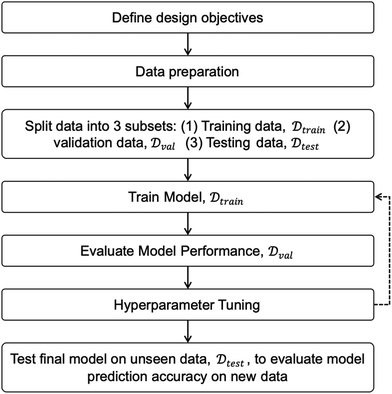
Tree-based methods are based on an application called decision-trees, which are algorithms that can solve both classification and regression problems for single output and multiple output problems.⁵⁷ The following characteristics of tree-based methods make them desirable for the application of this paper; (1) tree-based methods are interpretable and typically do not require feature standardization since these methods do not weigh the magnitude of feature vector values, (2) outliers are managed well in both the target and the features space, (3) these methods are able to be computationally scaled for larger datasets, (4) tree-based methods provide a good balance between model complexity and model.⁶³Fig. 5 illustrates the phases of building a ML model.

Fig. 5 Machine learning workflow.

The generated data is broken into subsets for training, validating and testing the ML model. Fig. 6 depicts how the dataset is typically split into the three subsets. Before tuning the ML model on all the data, it is customary practice to split the data into training, validation, and testing sets (samples of the larger dataset). The model trains on approximately 70% of the data. The model is then validated using the validation subset of data that it has never seen before. The process of training and validation is repeated for a defined number of iterations.

Fig. 6 Training, validation, and testing split.

Occasionally, when ML models learn from small datasets (<1000), hyperparameter tuning can quickly lead to overfitting or underfitting. This is especially true for tree-based methods trained on small datasets. k-Fold cross validation is used in the hyperparameter tuning stages to prevent overfitting. k-Fold cross validation repeats the process of splitting the dataset into training, validation, and testing five times; each iteration uses a different subset of data for training and validation. This method of cross validation assures that your dataset is generalizable. Referring to the ML flow diagram, the dataset is split into a training, testing, and validation data set. The k in k-fold cross validation refers to the number of validation folds (typically 5 or 10).

2.6 Machine learning model evaluation

The evaluation metric best suited for the applications in this paper is Mean Absolute Percentage Error (MAPE) which is defined in the following equation, where ŷ_i is the predicted value of the ith sample and n_samples is the number of samples.⁶⁴

The mean absolute percentage error (MAPE) is another risk metric used to evaluate regression problems. In the Python module scikit-learn, MAPE falls between zero and one. Values outside of this range suggest that the model is overfitting, underfitting, or the selected model may not be appropriate for the dataset and other models should be explored.⁶⁴

This equation will be used in the model evaluation process to determine how well the ML model will respond to new or unseen data. Lower errors mean that it is highly probable that the model will make good predictions on new data. High error metrics suggest that it is unlikely that the ML model is making accurate predictions on new data.

2.7 Constructing a machine learning based surrogate model

Surrogate modeling serves as a vital tool for approximating complex, non-interpretable (black box) ML or deep learning models, providing an affordable and interpretable alternative, denoted f̂. In the realm of engineering surrogate modeling, the strategy involves employing a comprehensible ML model to approximate an unknown function f. This approximation is achieved using a judiciously chosen subset of high-fidelity samples that effectively encapsulate the intricacies of the design space.

The machine learning methods utilized in surrogate modeling are not universally interpretable, and their complexity tends to escalate with an increasing number of features. Despite this, the application of surrogate models remains crucial in situations where understanding the underlying mechanisms is paramount.

Akin to the steps involved in developing a conventional ML model, surrogate modeling comprises several integral stages, each contributing to the overall efficacy of the process.

2.7.1 Computational data collection Benchmarked with physical laboratory results. The initiation phase involves the collection of computational data, aligning it with physical laboratory results for benchmarking. This ensures a congruence between simulated and real-world outcomes, laying a robust foundation for subsequent modeling.

2.7.2 Preliminary data-generation and feature-screening. Following data collection, preliminary steps encompass data generation and feature screening. This involves generating an initial dataset and screening features to identify those wielding significant influence on the target function, thereby streamlining subsequent analyses.

2.7.3 Data analysis and final feature selection. A meticulous data analysis procedure is then conducted to further refine the feature set. This stage aims to discern the most pertinent features, optimizing the model's accuracy and interpretability.

2.7.4 Sampling plan design. A critical aspect of the surrogate modeling process involves the design of an effective sampling plan. This entails planning the selection of data points, ensuring a judicious representation of the design space while maintaining computational efficiency.

2.7.5 Data-generation. Subsequent to the sampling plan, additional data points are generated to augment the dataset. This augmentation bolsters the model's capacity to capture complex relationships within the design space.

2.7.6 Machine learning modeling and evaluation. The crux of surrogate modeling lies in the application of ML techniques. Models are trained using the collected data to approximate the target function. Rigorous evaluation ensures the resultant model's accuracy and reliability.

2.7.7 ML model selection and surrogate model construction. The concluding phase involves the judicious selection of a suitable ML model, followed by the construction of the surrogate model (f̂). This step is pivotal in developing an interpretable model that effectively approximates the complex behavior of the original non-interpretable model f.

2.8. Multi-objective optimization to find a Pareto set of improved electrode designs

2.8.1 Multi-objective optimization and Pareto sets. After constructing an efficient and reliable ML based surrogate model, multi-objective optimization is employed to explore the surrogate model to find a Pareto set of optimal electrode designs. As discussed earlier, multi-objective optimization problems often have competing objectives. This problem maximizes VE, EE, and CE, which are calculated according to eqn (1)–(3). Next, the reasoning behind why a Pareto set of solutions is necessary for this specific problem is explained using a select few design parameters. For example, previous studies proved that cell efficiency can be improved by maximizing porosity and maximizing active surface area. With that said, increasing porosity inherently decreases active surface. This is due to the competing properties of the parameters causing a necessary tradeoff between the two. An increased porosity, while decreasing the mass transport resistance, has an indirect relationship with surface area causing an increased charge transfer resistance. Multi-objective optimization will account for the interactions between porosity, energy efficiency, coulombic efficiency, and voltage efficiency and provide a set of solutions that balances the tradeoffs between porosity and surface area.

2.8.2 Non-dominated sorting genetic algorithm II (NSGA-II). A non-dominated genetic sorting algorithm II (NSGA-II) is a variation of the genetic algorithm that is best suited to find a Pareto set of optimal solutions for multi-objective optimization problems. Similar to a traditional genetic algorithm, NSGA-II will begin with an initial population. The best design combinations in the initial population will move onto the second generation and this process will repeat until convergence. The main nuance to this approach is that each design combination is evaluated on its fitness score and the combinations are also ranked based on their location in the design domain. This eliminates the chance of having repetitive offspring in future generations as well as assuring that the entirety of the design space is explored.

2.9 Fabricated electrodes and their performance characterization

The microstructure of the base carbon cloth electrode (AvCarb 1071 HCBA) displays a bi-modal pore size distribution,⁴⁴ which is a critical feature allowing for lower mass transport resistances. Because of this, power density is improved, and pumping losses are reduced.⁴⁰ There are negligible effects of pumping power losses on the cell, leading to the omission of their effects in efficiency calculations. Larger pores of the electrode are responsible for delivering the electrolyte through convection, resulting in lower pumping power losses and the smaller pores allow for electrolyte diffusion to active sites which enhances reaction kinetics.^40,42 For this, AvCarb 1071 HCBA is chosen as the baseline for which machine learning suggestions will be implemented on. Based on the recommendations from the ML-based surrogate model, the binder-coated electrode (AvCarb T2314B) is prepared by adding a carbonaceous, porous binder layer to both sides of the AvCarb 1071 HCBA electrode. The electrodes, initially un-activated, are activated by heating in a furnace at 425 °C for 24 hours.

For evaluating the performance of the binder coated electrode (AvCarb T2314B), electrochemical testing is performed and compared amongst the baseline results for AvCarb 1071. The experimental setup uses a symmetric RFB cell with a 40 mL single tank of electrolyte which has been described in detail in the subsection “2.1 Experimental benchmarking of the computational model” of the Methodology section. One experiment performed consists of the baseline electrode (AvCarb 1071 HCBA), and the second experiment utilizes a binder-coated electrode (AvCarb T2314B). The overall compression ratio of the cell is around 41% for the experiment consisting of 1071 HCBA and around 49.7% when T2314B electrodes are used. EIS results are analyzed to quantify the resistance for direct comparison of electrode performance within a VRFB.

3. Results and discussion

3.1 Selected features

After identifying the initial set of features and completing the preliminary dataset generation, the final set of features is selected based on their impact on electrode functionality as well as the computational feasibility. The final set of features along with their lower and upper bounds are displayed in Table 3. Note that the fixed operating conditions in this study are current density set to be 1000 A m⁻² and flow rate set at 3.33 × 10⁻⁷ m³ s⁻¹.

Table 3 Final set of six selected features and their corresponding bounds

Parameter description	Lower bound	Upper bound
Porosity	0.7	0.97
Electric conductivity of the electrode (S m^−1)	60	110
Permeability of the electrode (m^2)	1 × 10^−10	5 × 10^−10
Mean pore diameter (m)	1 × 10^−4	1.2 × 10^−4
Average fiber diameter (m^2)	1 × 10^−5	2 × 10^−5
Cycle number	2	6

---

The bounds can also be written as shown in eqn (13) using porosity as an example.

σ^e ∈ [0.7, 0.97] (13)

The six features and their bounds shown in Table 3 describe the design domain. Please note that cycle number is an output of the computational model and may not be directly perceived as a statistical feature. However, it was used in training the ML algorithms and was deemed useful. Recalling that each feature, xⁱ, typically has lower and an upper bound constraints that needs to be specified, the feature vector, x, must be within the ML domain, represented by , which is a subset of all real numbers. is also a vector with m number of elements (features). This explanation is clearly summarized in eqn (14).⁶⁵

There are six selected features, but permeability is also not included in the sampling plan design since the permeability is calculated for each sample using the Carman–Kozeny equation. This equation relates the morphological parameters of porosity and average fiber diameter for each sample to calculate the permeability and can be shown below in eqn (15).⁶⁶

The response value of cycle number for each electrode design is recorded although it is not included in the sampling plan since it is technically a response that is output by the computational model. The porosity can be raised by the mean pore diameter depending on the pore sizes and the pore distribution in the material. Higher porosity can also be achieved by decreasing the fiber diameter to increase active surface area.

3.2 Latin hypercube sampling plan using quasi Monte-Carlo methods

The final statistical sampling plan consists of two hundred samples. This space filling sampling plan evenly distributes the two hundred samples throughout the design space. There are six selected features, but permeability is excluded from the sampling plan design as it is calculated using the other two features. Referring back to eqn (4), the sampling plan can be described using the matrix below where m = 5 and n = 200. m refers to each sample (observation) in the sampling plan.

Each sample in the LHS plan is an electrode design. Table 4 clearly outlines the first four electrode designs. For data visualization and ML model interpretability purposes, the mathematical notation displayed in Table 5 is used to describe the features and targets.

Table 4 The first four electrode designs created from the LHS sampling plan

Sample	σ ^e	ε	κ	d f	d p
m = 1	67.3	0.93	1.7 × 10^−10	1.4 × 10^−5	1.4 × 10^−4
m = 2	86.1	0.82	3.6 × 10^−11	1.9 × 10^−5	1.2 × 10^−4
m = 3	61.3	0.88	7.7 × 10^−11	1.8 × 10^−5	1.0 × 10^−4
m = 4	107.5	0.77	1.4 × 10^−11	1.7 × 10^−5	1.2 × 10^−4
m = 200	103.9	0.95	3.3 × 10^−10	1.4 × 10^−5	1.3 × 10^−4

---

Table 5 The notation used to define the electrode features and targets

Feature and target names	Symbol
Electrical conductivity of the electrode	σ ^e
Porosity	ε
Permeability	κ
Average fiber diameter	d f
Mean pore diameter	d p
Voltage efficiency	VE
Coulombic efficiency	CE
Energy efficiency	EE

---

Table 4 provides clear examples of what each electrode design (sample) from the LHS plan will look like. Each sample, n, has a selected value for electrical conductivity, porosity, permeability, average fiber diameter, and mean pore diameter.

The selected values fall between the lower and upper bounds assigned to each feature (shown in Table 3). The resulting distribution of values that the sampling plan created for each feature is shown in the Pairplot in Fig. 7. A Pairplot, or matrix of scatterplots, is used to show the distribution of samples for the features. The LHS plan using quasi-Monte-Carlo methods ensures that a representative subset of values is selected for each feature. The limited white space in each scatterplot in Fig. 7 shows that the sampling plan selected a representative subset of values for each feature. The permeability is calculated from d_f and ε. The script to generate the LHS plan with QMC methods considered four features; permeability is calculated using the Carman–Kozeny equation.⁶⁶ Therefore, sparse scatterplots in Fig. 7 can be attributed to permeability being a function of porosity and average fiber diameter.

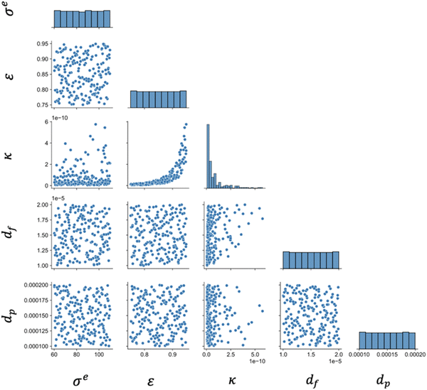Fig. 7 Feature distribution of the 200-point Latin hypercube sampling plan generated using QMC methods.

Table 4 displays the design combinations from the LHS sampling plan, which are displayed in Fig. 7. The numerical values for each of the five features for the first four electrode design combinations are displayed.

3.3 Dataset generation

3.3.1 Computational data-generation, results and charge–discharge curves. The computational time required to obtain cycling data for a single electrode design can range from 60 to 180 minutes. Simulating 200 samples would take over 300 hours to complete. An ample amount of time has been invested into collecting response results for all two hundred electrode designs. Due to the time-consuming nature of computational data-generation, an active learning approach is taken as data is collected. Active learning refers to re-training the ML models as the dataset is enriched with more samples.^{57,63,67–69} Since each sample has between 2 and 6 cycles and each cycle has three target values (VE, CE, EE), the final database has 387 fully labeled examples to support the data-driven modeling approaches. For each sample, the raw cycling data produced by the computational model is cleaned, renamed, and imported into MATLAB for plotting. Fig. 8 displays the charge–discharge curve produced when the computational model parameters are modified to match the electrode design specification of sample 4 (electrode design for sample 4 is shown in Table 4). The charging, discharging, and oscillating peaks are selected in MATLAB and the target values (EE, VE, CE) are calculated for each cycle.

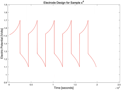Fig. 8 Charge–discharge curve plotted in MATLAB (refer to Table 4 for the electrode design details for sample 4 that produced this cycling curve).

3.3.2 Statistical analysis and data visualization. A Pairplot of the 387 fully labeled examples is provided in Fig. 9 which also includes cycle number, and the distribution of each target efficiency. The diagonal of the Pairplot contains histograms showing the distribution of collected values for each feature. Similar to Fig. 7, the axes labels are based on the mathematical notation displayed in Table 5.

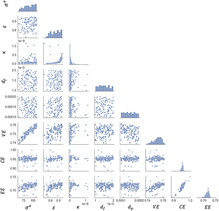Fig. 9 Pairplot (matrix of scatterplots) showing the feature and target distributions for the collected data from the sampling plan.

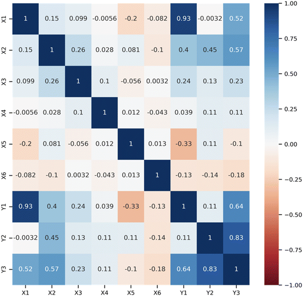
The Pearson correlation heatmap show that CE and VE are positively linearly correlated to EE with a correlation coefficient of r = 0.85 and r = 0.56, respectively. All three efficiency values are linearly related to porosity. The voltage and coulombic efficiency trends can be summarized by the energy efficiency target. The one exception is that VE is linearly related to σ^e with r = 0.93. The Pearson correlation coefficients correlation coefficients summarized in Fig. 10 offer a thorough understanding of the design space and will guide machine learning model selection. The lack of linear feature-target correlations indicates that simple linear regression techniques are unable to capture the complex non-linear relationships.

Fig. 10 Pearson correlation coefficient heatmap.

3.3.3 Understanding the generated response data (EE, CE, VE). Generated response data, shown in Fig. 11, highlights the similarities and differences between the ranges of values for each response variable. The range of values obtained for CE is between 90–98%, which is comparable to the experimentally obtained values. The minimum and maximum efficiency values for the three target variables is also outlined in Table 6.

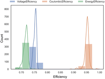Fig. 11 Histogram and kernel density estimates (KDEs) containing the distribution of values collected for the three response variables, VE, CE, and EE.

Table 6 Minimum and maximum efficiency values for each target

	VE	CE	EE
Minimum (%)	78.94	89.02	67.61
Maximum (%)	76.15	99.85	75.04

---

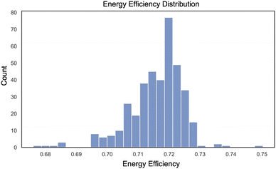
A more refined, higher resolution histogram for the EE has been provided below in Fig. 12. The relatively wide range of values (ranges from 0.68 to 0.75) obtained is an indication of the relatively large potential improvements on the energy efficiency that can be obtained with an optimized electrode design.

Fig. 12 Energy efficiency distribution emphasizing the percentage range for improvement.

3.4 Machine learning model development

3.4.1 Machine learning model selection. Initially, since the EE target contains the VE and CE information, single output machine learning models were trained to determine what models are suitable for this problem. This approach also reduces the complexity of the model which in turn reduces the computational power necessary to train, validate, and test each model. A preliminary test was performed using the Automated regression model selection with bayesian optimization tool in MATLAB, fitting the regression models to the single response value of energy efficiency. This tool automatically trains and evaluates several regression models with various hyperparameters and returns corresponding models and hyperparameters with the highest prediction accuracy. The computing time is approximately 45 minutes. This process pinpoints appropriate regression models to fit this dataset as opposed to manually evaluating every regression algorithm. Although the automated regression model selection with Bayesian optimization is performed as a multivariate regression problem with a single output, the single output of EE encompasses the CE and VE information therefore no information is lost. The results suggested that tree-based ensemble methods, specifically random forests, would be the most suitable for this dataset. Therefore, the ML models selected for further investigation are random forest regressors and gradient boosting regressors, both of which are tree-based ensemble methods.

3.4.2 Comparing feature importance scores for single and multiple output random forest regression models. Once the single output and multiple output random forest regressors (RFRs) are trained and evaluated, the feature importance scores are found. Table 7 outlines which target variables each ML model was trained on. For example, ML Model 1 is trained to predict VE. Model 4 is the multiple output model which is trained on all three target variables (VE, CE, and EE).

Table 7 Using the mathematical notation to define the target variable for each model

Model	Target values
Model 1	VE
Model 2	CE
Model 3	EE
Model 4	VE, CE, EE

---

The feature importance analysis conducted for all the baseline RFR models reveal that the features in Model 3 and Model 4 have approximately the same importance scores. Model 2 follows similar trends when compared to Model 3 and Model 4. Model 1, where the target value is VE, has a noticeably different distribution of feature importance scores. Model 1 heavily relies on conductivity, whereas the other models rely more so on porosity. The comparisons of the four models can be seen in Fig. 13 and Table 8.

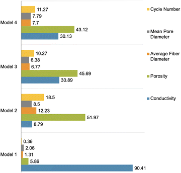Fig. 13 Feature importance scores for single and multiple output random forest regression models (models 1, 2, 3, and 4).

Table 8 Feature importance scores for single and multiple output random forest regression models

Feature importance scores
	Model 1	Model 2	Model 3	Model 4
Conductivity	90.41	8.79	30.89	30.13
Porosity	5.86	51.97	45.69	43.12
Average fiber diameter	1.31	12.23	6.77	7.7
Mean pore diameter	2.06	8.5	6.38	7.79
Cycle number	0.36	18.5	10.27	11.27

---

The single output models are prone to overfitting, a tell-tale sign of overfitting is if the testing error is larger than the training error.^70–72 The single output models also did not account for certain inherent physical limitations that can be accounted for when using a multiple objective model. The best performing ML models that will be used as surrogate models are a multiple output gradient boosting regressor and a multi-output RFR.

3.5 ML based surrogate models

The best performing ML models are then used to construct the surrogate models. The top two ML models along with their training and testing error are shown in this section. Two ML methods to support surrogate modeling were selected as opposed to one method considering that as the database expands, RFR will perform slower while the GBRs will maintain fast training and evaluation times. The best performing models will be referred to as Model 1 and Model 2, where Model 1 is the multi-output RFR and Model 2 is the multi-output GBR. RFRs are less complex than GBRs and therefore more prone to overfitting during the hyperparameter tuning process. The following hyperparameter tuning methods were performed on Model 1 and Model 2 to achieve maximum model performance: exhaustive grid search over all specified parameters, randomized grid search, and hyperparameter tuning using Bayesian optimization. (These hyperparameter tuning techniques were performed in the python software's scikit-learn and optuna). The process of k-fold cross validation was performed with five folds to determine whether the hyperparameters were causing over or under fitting. Model 1 performed the best with the default scikit-learn hyperparameters. Model 2 performance increased when implementing hyperparameter tuning strategy using Bayesian optimization. Fig. 14 displays the resulting training and testing error for the tuned surrogate models. The MAPE scoring metric is used as it is the most interpretable.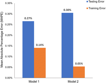

Fig. 14 Multi-output RFR; model 2: multi-output GBR – training and testing scores using mean absolute percentage error (MAPE) scoring metric.

The MAPE values in Fig. 14 show that the surrogate models prediction errors are less than 0.15% on the training dataset. The testing error is slightly higher, though still less than 0.3%. The model does not show evidence of overfitting, if the testing error is not excessively higher than the training error.

To further emphasize the validity using k-fold cross validation, the final hyperparameters for the multi-output random forest regressor are shown in Table 9 where MAPE remains low for all five folds.

Table 9 Hyperparameter tuning results for the multi-output random forest regressor

Hyperparameter description	Hyperparameter value
mean_fit_time	0.429506
std_fit_time	0.009786
mean_score_time	0.028945
std_score_time	0.001787
param_estimator__max_depth	33
param_estimator__max_features	None
param_estimator__min_samples_leaf	2
param_estimator__min_samples_split	7
split0_test_score	0.480926
split1_test_score	−0.064334
split2_test_score	0.678854
split3_test_score	0.39821
split4_test_score	0.331645
mean_test_score	0.36506
std_test_score	0.24433
rank_test_score	1

---

3.6 Multi-objective optimization with NSGA-II results

A non-dominated genetic sorting algorithm II (NSGA-II) is a variation of the genetic algorithm that is best suited to find a Pareto set of optimal solutions for multi-objective optimization problems. Like a traditional genetic algorithm, NSGA-II will begin with an initial population, P. The best design combinations in the initial population will move onto the second generation and this process will repeat until convergence.

The main nuance to this approach is that each design combination is evaluated on its fitness score and the combinations are also ranked based on their location in the design domain. This will eliminate the chance of having repetitive offspring in future generations as well as assuring that the entirety of the design space is explored. The final electrode design parameters for surrogate Model 1 and 2 using NSGA-II are listed in Table 10. The multiple objective optimization with 5 inputs (x¹, x², x³, x⁴, x⁵) and 3 outputs (f₁, f₂, f₃) = (CE, VE, EE) using the NSGA-II, the optimization problem can be represented as follows: the objective function is represented by eqn (17) and the decision variables are σ^e, κ, ε, d_f, d_p shown as x.

Table 10 Resulting electrode design parameters for surrogate Model 1 and surrogate Model 2 using NSGA-II for multi-objective optimization

	Surrogate Model 1	Surrogate Model 2
Iteration number	227	212
Electrical conductivity (S m^−1)	106.4	107.4
Porosity	0.799	0.900
Permeability (m^2)	8.1 × 10^−10	5.71 × 10^−10
Average fiber diameter (m)	1.2 × 10^−5	1.4 × 10^−5
Mean pore diameter (m)	1.11 × 10^−4	1.85 × 10^−4
Predicted voltage efficiency	75.75%	75.70%
Predicted coulombic efficiency	96.10%	95.72%
Predicted energy efficiency	73.12%	72.52%

---

The objective functions from eqn (17) are then evaluated for each solution P. The solutions are ranked based on non-domination, each solution is assigned to a front, the crowding distance for solutions in each front is found. The parents for the next generation are selected abased on the non-dominated fronts and crowding distance. Generic operations are applied to create offspring solutions.

The parents of the offspring form a new population. This process continues to repeat until termination criteria are met.⁷³ The general trend obtained using the ML-based screening and optimization tool suggests that mean pore diameter should be reduced compared to the tested carbon cloth electrodes while maintaining a similar permeability value. Based on this suggestion, a new type of carbon cloth electrode has been fabricated by introducing a carbonaceous binder into woven fabric to make hydrophilic cloths with more complex pore structure and reduced mean pore diameter.

To evaluate the performance of the VRFB with each electrode, ASR values were quantified and compared to visualize the effects of adding a binder to the carbon cloth electrode. Ohmic, charge transfer, and mass transport resistances are determined through curve fitting of the EIS plots, which can be seen in Fig. 15a. It is known that the left-most intersection point on the x-axis demonstrates the ohmic resistance for the recorded cycle, the diameter of the first semi-circle of an EIS plot represents charge transfer resistance, and the diameter of the second semi-circle corresponds to mass transport resistance when reading the plot from left to right. Using a Z-fit curve fitting analysis within EC-Lab software, the Randles equation is utilized which represents the circuit of the physical system. This equation is commonly used to interpret impedance data and confirm the values of corresponding resistances obtained from the semi-circle intersection points.⁷⁴Fig. 15b below displays the comparison of associated resistance values throughout the duration of the symmetric cell experiments.

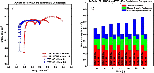Fig. 15 (a) EIS data from the beginning and end of each experiment and (b) comparison of total resistance values of the VRFB with AvCarb 1071 HCBA and AvCarb T2314B electrodes.

Fig. 15b illustrates the comparative analysis of electrode resistances, showcasing the superior performance of the novel binder-coated electrode over the standard 1071 HCBA electrode. Symmetric cell cycling coupled with EIS provides a direct correlation of the performance enhancement of the electrode. A constant SOC symmetric cell experiment is advantageous for multiple reasons, such as the mitigation of cross-over of the active species and the absence of chemical or electrical potential gradients which makes the effects of side reactions negligible.^44,75 Resistance data from the analysis of EIS experiments can then be used to quantify the performance of the electrode itself without concern for the effects of electrolyte degradation. The performance enhancement of the VRFB with the new electrodes is evidenced by the reduction in both ohmic and mass transport resistances by 24% and 66% respectively, attributed to modifications in the electrode's microstructural parameters induced by the binder coating. However, it is critical to note the observed increase in charge transfer resistance, which can be attributed to the suboptimal activation conditions for the newly fabricated electrodes, underscoring the preliminary nature of these findings. The AvCarb T2314B electrode underwent 24 hours of thermal activation in a furnace at a temperature of 425 °C as an initial activating condition. An in-depth investigation focused on refining these thermal activation conditions is currently underway, promising to address this limitation and reduce charge transfer resistance.

The aforementioned enhancements in mass transport, ohmic, and total resistance values signify a marked improvement in carbon cloth electrode performance within VRFB applications. EIS experiments, performed to compare the base electrode, AvCarb 1071 HCBA, and the electrode with the addition of a porous binder, AvCarb T2314B, display promising results utilizing the newly fabricated electrode in terms of reduced total ASRs. These findings corroborate the hypothesis that integrating a carbonaceous, porous binder layer—as recommended by our optimization analysis—substantially benefits VRFB performance. Such findings not only highlight the critical role of electrode composition and structure in optimizing battery performance but also open avenues for future research to unlock the full potential of VRFB technologies.

4. Conclusion

In summary, this research makes a substantial contribution to the field by introducing a cost-effective modeling strategy aimed at optimizing the design of porous carbon cloth electrodes for VRFB technology. The key innovation lies in the development of a versatile framework that allows for the selection and application of optimal machine learning techniques tailored to the unique challenges of the design problem. With operating conditions in RFB systems being user-defined and varying case by case, the behavior of porous carbon electrodes exhibits significant complexity contingent on specific operational scenarios. Given the impracticality of creating an exhaustive model for every operating condition, our proposed cost-effective framework offers a customizable surrogate modeling solution, maintaining high prediction accuracy while ensuring computational efficiency.

Crucially, the adaptability of our framework positions it as a valuable tool for both single- and multi-objective optimization problems, enabling the discovery of improved electrode design combinations under the specified operating conditions outlined in the case study. The novel electrode design not only reduces average ohmic and mass transport resistances but also results in a reduction to the overall increase of total resistances from 29% to 0.4% during the 24-hour constant SOC symmetric cycling experiment. It is noteworthy that ongoing experimental results, set to be disclosed soon, will provide additional empirical insights, further validating the robustness and applicability of our proposed framework. This study not only represents a significant step forward but also lays the groundwork for future investigations, offering a platform for discovering enhanced electrode combinations tailored to specific operating conditions, thereby eliminating the need for extensive laboratory testing or substantial computational resources. By addressing the nuanced challenges of electrode design and optimization, this work paves the way for significant advancements in energy storage solutions, catering to the growing global demand for renewable energy integration and grid stabilization.

Author contributions

Alina Berkowitz: data curation, formal analysis, writing original draft. Ashley A. Caiado: data curation, formal analysis, writing – original draft. Sundar Rajan Aravamuthan: formal analysis, writing – review & editing. Aaron Roy: conceptualization, resources, supervision, writing – review & editing. Ertan Agar: conceptualization, supervision, funding acquisition, writing – review & editing. Murat Inalpolat: conceptualization, supervision, funding acquisition, writing – review & editing.

Nomenclature

ε	Porosity
d f	Average fiber diameter, m^2
κ	Permeability, m^2
d p	Mean pore diameter, m
K CK	Kozeny–Carman coefficient
σ ^e	Electrical conductivity of porous carbon electrode, S m^−1
I	Current density, A m^−2
Φ	Potential, V
V^3+	V(III)
VO^2+	V(IV)
VO2^+	V(V)
kW h	Kilowatt hour
Anode	Positive electrode
Cathode	Negative electrode
R ^2	Coefficient of determination
y	Data label (response)
n	Discrete number of observations
	Domain (machine learning)
f	Expensive “black-box” function
f̂	Surrogate model (emulator or meta-model)
X	Data matrix
m	Number of samples
n	Number of design variables (features)
x ^i	m-Dimensional feature vector
{xi, yi}	Data pairs
	Training dataset
	Validation dataset
	Testing dataset
σ	Standard deviation
σ ^2	Variance
μ	Mean
σ	Standard deviation
t d	Charging time, s
t c	Discharging time, s
V ave,d	Average discharging voltage, V
V ave,c	Average charging voltage, V
k	Number of folds when using k-fold cross validation
R ohmic	Ohmic resistances
R ct	Charge transfer resistances
R mt	Mass transport resistances
ML	Machine learning
VE	Voltage efficiency
EE	Energy efficiency
CE	Coulombic efficiency
MAPE	Mean absolute percentage error
MAPD	Mean absolute percentage deviation (same as MAPE)
GBR	Gradient boosting regressor
RFR	Random forest regressor
LHS	Latin hypercube sampling
QMC	Quasi Monte-Carlo
KDE	Kernel density estimation
OCV	Open circuit voltage
MSE	Mean squared error
MAE	Mean absolute error
RMSE	Root mean squared error
r	Pearson correlation coefficient (between −1 and +1)

Data availability

(i) The original COMSOL model can be requested from K. W. Knehr, Ertan Agar and E. C. Kumbur, the corresponding authors of ref. 28. Available at https://iopscience.iop.org/article/10.1149/2.017209jes/meta. (ii) The optimisation steps are detailed in the source code for the GBR and RFR model. The reference for the source code is as follows: A. Berkowitz, 2024, VRFB-Electrode-Optimization, https://doi.org/10.5281/zenodo.12702156. (iii) The data for the experimentally validated computational model, which supports the data-driven modelling approach are detailed in ref. 28, 29, 55 and are available at https://iopscience.iop.org/article/10.1149/2.017209jes/meta, https://doi.org/10.1016/j.electacta.2013.03.030 and https://doi.org/10.1016/j.jpowsour.2013.08.023, respectively.

Conflicts of interest

There are no conflicts to declare.

Acknowledgements

This material is based upon work supported by the U.S. Department of Energy's Office of Energy Efficiency and Renewable Energy (EERE) under the Advanced Manufacturing Office, award number DE-EE0009102. Any opinions, findings, and conclusions or recommendations expressed in this material are those of the author(s) and do not necessarily reflect the views of the Department of Energy. The authors are also indebted to AvCarb Material Solutions for providing carbon electrodes and insightful discussions.

References

1. J. Kerry, The Long-Term Strategy of the United States, Pathways to Net-Zero Greenhouse Gas Emissions by 2050, 2021. p. 65.
2. What is U.S. electricity generation by energy source? 2023; Available from: https://www.eia.gov/tools/faqs/faq.php?id=427&t=3.
3. L. Chang and Z. Wu, Performance and Reliability of Electrical Power Grids under Cascading Failures, Int. J. Electrical Power Energy Systems, 2011, 33, 1410–1419.
4. P. Dey, et al., Impact of Topology on the Propagation of Cascading Failure in Power Grid, IEEE Trans. Smart Grid, 2016, 7(4), 1970–1978.
5. B. J. van Ruijven, E. De Cian and I. Sue Wing, Amplification of future energy demand growth due to climate change, Nat. Commun., 2019, 10(1), 2762.
6. A.-G. Jimoh and J. L. Munda, Challenges of Grid Integration of Wind Power on Power System Grid Integrity: A Review, Int. J. Renewable Energy Res., 2013, 2.
7. S. K. Pahari, et al., Designing high energy density flow batteries by tuning active-material thermodynamics, RSC Adv., 2021, 11(10), 5432–5443.
8. M. S. Ziegler, et al., Storage Requirements and Costs of Shaping Renewable Energy Toward Grid Decarbonization, Joule, 2019, 3(9), 2134–2153.
9. M. Mann, et al., Energy Storage Grand Challenge Energy Storage Market Report, D.o, Energy, 2020, 65.
10. G. P. Wheeler, L. Wang and A. C. Marschilok, Beyond Li-ion Batteries for Grid-Scale Energy Storage, Cambridge University Press, Cambridge, 2022.
11. J. Arteaga, H. Zareipour and V. Thangadurai, Overview of Lithium-Ion Grid-Scale Energy Storage Systems, Curr. Sustainable/Renewable Energy Rep., 2017, 4, 1–12.
12. N. Collath, et al., Aging aware operation of lithium-ion battery energy storage systems: a review, J. Energy Storage, 2022, 55, 105634.
13. M. Bragard, et al., The Balance of Renewable Sources and User Demands in Grids: Power Electronics for Modular Battery Energy Storage Systems, Power Electron., IEEE Trans., 2011, 25, 3049–3056.
14. Z. Yang, et al., Electrochemical Energy Storage for Green Grid, Chem. Rev., 2011, 111(5), 3577–3613.
15. J. Mitali, S. Dhinakaran and A. A. Mohamad, Energy storage systems: a review, Energy Storage Sav., 2022, 1(3), 166–216.
16. A. Z. Weber, et al., Redox flow batteries: a review, J. Appl. Electrochem., 2011, 41(10), 1137–1164.
17. E. Sánchez-Díez, et al., Redox flow batteries: Status and perspective towards sustainable stationary energy storage, J. Power Sources, 2021, 481, 228804.
18. G. L. Soloveichik, Flow Batteries: Current Status and Trends, Chem. Rev., 2015, 115(20), 11533–11558.
19. Z. Li, et al., Air-Breathing Aqueous Sulfur Flow Battery for Ultralow-Cost Long-Duration Electrical Storage, Joule, 2017, 1(2), 306–327.
20. M. Nourani, et al., Elucidating Effects of faradaic Imbalance on Vanadium Redox Flow Battery Performance: Experimental Characterization, J. Electrochem. Soc., 2019, 166(15), A3844–A3851.
21. V. Viswanathan, et al., Cost and performance model for redox flow batteries, J. Power Sources, 2014, 247, 1040–1051.
22. R. M. Darling, et al., Pathways to low-cost electrochemical energy storage: a comparison of aqueous and nonaqueous flow batteries, Energy Environ. Sci., 2014, 7(11), 3459–3477.
23. J. Houser, et al., Architecture for improved mass transport and system performance in redox flow batteries, J. Power Sources, 2017, 351, 96–105.
24. Energy Storage Grand Challenge Roadmap, D.o. Energy, Editor. 2020.
25. I. Gyuk, et al., Grid energy storage, US Department of Energy, 2013.
26. M. Skyllas-Kazacos, et al., Recent advances with UNSW vanadium-based redox flow batteries, Int. J. Energy Res., 2010, 34(2), 182–189.
27. C. R. Dennison, et al., Enhancing Mass Transport in Redox Flow Batteries by Tailoring Flow Field and Electrode Design, J. Electrochem. Soc., 2016, 163(1), A5163.
28. K. Knehr, et al., A Transient Vanadium Flow Battery Model Incorporating Vanadium Crossover and Water Transport through the Membrane, J. Electrochem. Soc., 2012, 159, A1446–A1459.
29. E. Agar, et al., Species transport mechanisms governing capacity loss in vanadium flow batteries: Comparing Nafion® and sulfonated Radel membranes, Electrochim. Acta, 2013, 98, 66–74.
30. Q. He, et al., Modeling of Vanadium Redox Flow Battery and Electrode Optimization with Different Flow Fields, e-Prime, 2021, 1, 100001.
31. K. J. Kim, et al., A technology review of electrodes and reaction mechanisms in vanadium redox flow batteries, J. Mater. Chem. A, 2015, 3(33), 16913–16933.
32. A. Forner-Cuenca, et al., Exploring the Role of Electrode Microstructure on the Performance of Non-Aqueous Redox Flow Batteries, J. Electrochem. Soc., 2019, 166(10), A2230.
33. F. Chu, et al., Novel Interdigitated Flow Field with a Separated Inlet and Outlet for the Vanadium Redox Flow Battery, Energy Fuels, 2023, 37(16), 12166–12177.
34. M.-Y. Lu, et al., A novel rotary serpentine flow field with improved electrolyte penetration and species distribution for vanadium redox flow battery, Electrochim. Acta, 2020, 361, 137089.
35. J. Jang, et al., Carbon cloth modified by direct growth of nitrogen-doped carbon nanofibers and its utilization as electrode for zero gap flow batteries, Chem. Eng. J., 2024, 481, 148644.
36. H. R. Jiang, et al., A uniformly distributed bismuth nanoparticle-modified carbon cloth electrode for vanadium redox flow batteries, Appl. Energy, 2019, 240, 226–235.
37. Z. He, et al., Modified carbon cloth as positive electrode with high electrochemical performance for vanadium redox flow batteries, J. Energy Chem., 2016, 25(4), 720–725.
38. Z. Zhang, et al., A composite electrode with gradient pores for high-performance aqueous redox flow batteries, J. Energy Storage, 2023, 61, 106755.
39. X. L. Zhou, et al., A highly permeable and enhanced surface area carbon-cloth electrode for vanadium redox flow batteries, J. Power Sources, 2016, 329, 247–254.
40. A. Forner-Cuenca, et al., Exploring the Role of Electrode Microstructure on the Performance of Non-Aqueous Redox Flow Batteries, J. Electrochem. Soc., 2019, 166(10), A2230–A2241.
41. M. Nourani, et al., Exploring the Structure-Function-Performance Relationship of Carbon Electrodes Toward Rational Design of High-Performance Redox Flow Cells, ECS Meeting Abstracts, 2021, MA2021-01(3), 215.
42. K. M. Tenny, et al., Comparing Physical and Electrochemical Properties of Different Weave Patterns for Carbon Cloth Electrodes in Redox Flow Batteries, J. Electrochem. Energy Convers. Storage, 2020, 17(4), 041010.
43. M. Nourani, et al., Impact of Corrosion Conditions on Carbon Paper Electrode Morphology and the Performance of a Vanadium Redox Flow Battery, J. Electrochem. Soc., 2019, 166(2), A353–A363.
44. A. A. Caiado, et al., Exploring the Effectiveness of Carbon Cloth Electrodes for All-Vanadium Redox Flow Batteries, J. Electrochem. Soc., 2023, 170(11), 110525.
45. B. A. Simon, et al., Combining electrochemical and imaging analyses to understand the effect of electrode microstructure and electrolyte properties on redox flow batteries, Appl. Energy, 2022, 306, 117678.
46. X. Ma, H. Zhang and F. Xing, A three-dimensional model for negative half cell of the vanadium redox flow battery, Electrochim. Acta, 2011, 58, 238–246.
47. E. Ali, et al., A numerical study of electrode thickness and porosity effects in all vanadium redox flow batteries, J. Energy Storage, 2020, 28, 101208.
48. C. Yin, et al., Three dimensional multi-physical modeling study of interdigitated flow field in porous electrode for vanadium redox flow battery, J. Power Sources, 2019, 438, 227023.
49. D. You, H. Zhang and J. Chen, A simple model for the vanadium redox battery, Electrochim. Acta, 2009, 54(27), 6827–6836.
50. G. Zhang, et al., Optimization of porous media flow field for proton exchange membrane fuel cell using a data-driven surrogate model, Energy Convers. Manage., 2020, 226, 113513.
51. M. Kok, A. Khalifa and J. Gostick, Multiphysics Simulation of the Flow Battery Cathode: Cell Architecture and Electrode Optimization, J. Electrochem. Soc., 2016, 163, A1408–A1419.
52. S. Wan, et al., A coupled machine learning and genetic algorithm approach to the design of porous electrodes for redox flow batteries, Appl. Energy, 2021, 298, 117177.
53. Product Page (Fabric). [cited 2022 November 10]; Available from: https://www.avcarb.com/product-page-fabric/.
54. E. Agar, et al., Reducing capacity fade in vanadium redox flow batteries by altering charging and discharging currents, J. Power Sources, 2014, 246, 767–774.
55. COMSOL Multiphysics, COMSOL AB, Stockholm, Sweden, 2024.
56. MATLAB, The MathWorks Inc., Natick, Massachusetts, 2022.
57. A. Géron, Hand-On Machine Learning with Scikit-Learn, Keras, and TensorFlow: Concepts, Tools, and Technoques to Build Intelligent Systems, 2 edn, 2019.
58. C. M. Bishop, Pattern Recognition and Machine Learning, Springer, New York, 2006.
59. C. Kamath, Intelligent sampling for surrogate modeling, hyperparameter optimization, and data analysis, Mach. Learn. Appl., 2022, 9, 100373.
60. W. J. Morokoff and R. E. Caflisch, Quasi-Random Sequences and Their Discrepancies, SIAM J. Sci. Comput., 1994, 15(6), 1251–1279.
61. N. Packham and W. Schmidt, Latin hypercube sampling with dependence and applications in finance, J. Comput. Finance, 2010, 13, 81–111.
62. H. Mahmoudi and H. Zimmermann, A new sampling technique for Monte Carlo-based statistical circuit analysis, 2017, pp. 1277–1280.
63. T. J. Hastie, R. Tibshirani and J. H. Friedman, The Elements of Statistical Learning, 2001.
64. F. Pedregosa, et al., Scikit-learn: Machine Learning in Python, J. Mach. Learn. Res., 2011, 12, 2825–2830.
65. A. Forrester, A. Sobester and A. Keane, Engineering Design Via Surrogate Modelling: A Practical Guide, 2008.
66. Z. Cheng, et al., Data-driven electrode parameter identification for vanadium redox flow batteries through experimental and numerical methods, Appl. Energy, 2020, 279, 115530.
67. B. Settles, Active Learning, 2012, vol. 6.
68. P. Ren, et al., A Survey of Deep Active Learning, ACM Comput. Surv., 2021, 54(9), 180.
69. B. Settles, From Theories to Queries: Active Learning in Practice, in Active Learning and Experimental Design workshop In conjunction with AISTATS 2010, ed. G. Isabelle, et al., PMLR: Proceedings of Machine Learning Research, 2011, pp. 1–18.
70. T. Regan, et al., Wind Turbine Blade Damage Detection Using Various Machine Learning Algorithms. in ASME 2016 International Design Engineering Technical Conferences and Computers and Information in Engineering Conference, 2016.
71. J. Solimine and M. Inalpolat, An unsupervised data-driven approach for wind turbine blade damage detection under passive acoustics-based excitation, Wind Eng., 2022, 46(4), 1311–1330.
72. T. Regan, C. Beale and M. Inalpolat, Wind Turbine Blade Damage Detection Using Supervised Machine Learning Algorithms, J. Vibration Acoustics, 2017, 139(6), 1–14.
73. K. Deb, et al., A Fast Elitist Non-dominated Sorting Genetic Algorithm for Multi-objective Optimization: NSGA-II. Parallel Problem Solving from Nature PPSN VI, Springer Berlin Heidelberg, Berlin, Heidelberg, 2000.
74. I. D. Raistrick, J. R. Macdonald and D. R. Franceschetti, Theory, Impedance Spectrosc., 2018, 21–105.
75. R. A. Potash, et al., On the Benefits of a Symmetric Redox Flow Battery, J. Electrochem. Soc., 2016, 163(3), A338.

---