DOI:
10.1039/D2GC04425K
(Paper)
Green Chem., 2023,
25, 3475-3492
Accurate prediction of carbon dioxide capture by deep eutectic solvents using quantum chemistry and a neural network†
Received
22nd November 2022
, Accepted 22nd February 2023
First published on 28th February 2023
Abstract
Carbon dioxide (CO2) emissions from fossil fuel combustion are a significant source of greenhouse gas, contributing in a major way to global warming and climate change. Carbon dioxide capture and sequestration is gaining much attention as a potential method for controlling these greenhouse gas emissions. Among the environmentally friendly solvents, deep eutectic solvents (DESs) have demonstrated the potential capability for carbon capture. To establish a theoretical framework for DES activity, thermodynamics modeling and solubility predictions are significant factors to anticipate and understand the system behavior. Here, we combine the COSMO-RS model with machine learning techniques to predict the solubility of CO2 in various deep eutectic solvents. A comprehensive data set was established comprising 1973 CO2 solubility data points in 132 different DESs at a variety of temperatures, pressures, and DES molar ratios. This data set was then utilized for the further verification and development of the COSMO-RS model. The CO2 solubility (ln(xCO2)) in DESs calculated with the COSMO-RS model differs significantly from the experiment with an average absolute relative deviation (AARD) of 23.4%. A multilinear regression model was developed using the COSMO-RS predicted solubility and a temperature-pressure dependent parameter, which improved the AARD to 12%. Finally, a machine learning model using COSMO-RS-derived features was developed based on an artificial neural network algorithm. The results are in excellent agreement with the experimental CO2 solubilities, with an AARD of only 2.72%. The ML model will be a potentially useful tool for the design and selection of DESs for CO2 capture and utilization.
1. Introduction
Carbon dioxide (CO2) emissions are a major source of global greenhouse gas and therefore a cause of global warming, spurring the scientific community to focus on CO2 capture.1 Recent atypical changes in the global climate are most likely the result of an increase in anthropogenic greenhouse gas (GHG) emissions, particularly carbon dioxide (CO2), which began in the preindustrial era. As a result of global warming, we are witnessing an increase in the frequency and severity of extreme weather events (global temperature, sea levels, floods, droughts, rainfall pattern changes) and the spread of infectious diseases.2 An increase of up to 5 °C in surface temperature is predicted as a result of continuous GHG emissions together with long-lasting climate change, posing a severe and irreversible risk to humanity and ecosystems.3–5 The Intergovernmental Panel on Climate Change (IPCC) estimates that nearly 80% of all CO2 emissions are caused by fossil fuels and minerals used in the production of electricity.6 According to Earth's CO2 observatory, the average atmospheric CO2 concentration has increased dramatically, from 172 to 300 parts per million (ppm) before the most recent industrial era to 416.47 ppm on May 30, 2020.7 The International Energy Agency (IEA) reported that in 2021, global CO2 emissions reached an all-time high of 36.3 gigatons (Gt), an increase of 6% from 2020.8 The Paris Accord of 2015, which was signed by 195 nations, declared “carbon-neutrality” as a global goal for a sustainable future, and the dominant nations and regions (such as the United States of America, China, Japan, and Europe) have proposed their targets and plans. To date, numerous techniques (such as sequestration, utilization, and capture) have been developed to lower CO2 emissions.7,9
There are several different technologies that are being investigated for the capture of CO2, for example, pressure-swing adsorption and physical or chemical-solvent scrubbing.7,10 However, most technologies still suffer from high energy requirements, increased costs, and significant secondary pollution as a result of the complexity of the gas components.7,11 There is therefore a pressing need for the development of new capture technologies, which may include the design of new solvents and novel processes. Ionic liquids (ILs) are among the potential solvents for CO2 capture12,13 and have been extensively studied due to their unique and attractive properties.13–15 However, due to the extensive procedures and multiple steps involved in the synthesis and purification process, ILs are expensive solvents. For this reason, deep eutectic solvents (DESs) have emerged as promising alternatives to ILs in a wide variety of research areas and industries, including CO2 capture, biomass processing, nanotechnology, extraction processes, electrochemistry, catalysts, etc.16,17
DESs are unique solvents with many desirable characteristics, including low vapor pressure, high conductivity, high thermal and chemical stability, non-flammability, non-toxicity and a large chemical window.18,19 When compared to ILs, DESs offer a few primary advantages, the most notable of which is that the preparation of DESs is simple and economical, and there is no additional purification step required.18,20 The most fascinating property of DESs is their structural diversity. DESs are prepared by mixing a hydrogen bond acceptor (HBA) and hydrogen bond donor (HBD) at a specific molar ratio, and the resulting mixture turns into a liquid that is driven by strong interactions between HBA and HBD.20,21 A large number of cheap and renewable compounds can serve as the HBA (e.g., [Ch]Cl) and HBD (e.g., urea, sugars, acids, etc.), making DESs more affordable and sustainable than ILs.17
In recent years, DESs have been demonstrated as a potential solvent for CO2 absorption.5,22,23 However, to date the majority of the research into CO2 absorption using DESs has relied on experimental methods, which have only been able to address a small fraction of potential DES candidates.24,25 Because of structural diversity, there are approximately 1018 DES combinations that can be used to design a solvent with potentially improved CO2 absorption capabilities.26 The experimental screening of such a large number of combinations for their capacity to solubilize CO2 is intractable. Therefore, in this context, it is highly desirable and emerging to have a reliable computational model for predicting CO2 solubilities in DESs. This would reduce both the cost and the time required to develop effective solvent systems for carbon capture and utilization.
In recent years, a variety of thermodynamic models such as NRTL (non-random two-liquid), UNIQUAC (UNIversal QUAsiChemical), and UNIFAC (UNIQUAC Functional-group Activity Coefficients)27 and equation of state methods (i.e., PC-SAFT (perturbed chain-statistical associating fluid theory),28 soft-SAFT,29 CPA (Cubic-Plus Association),30 and PR-EoS (Peng-Robinson equation of state30,31) have been successfully implemented in DES-containing systems for the purpose of predicting gas solubility. However, these methods require experimental input data to fit molecule-specific binary interaction and mixing parameters, which limits the applicability space for novel solvent systems such as ILs and DESs. Recently, Biswas (2022)32 performed molecular dynamics (MD) simulations of CO2 in ionic liquids (ILs). Also using MD, Wang et al. (2019)33 studied the interaction of phosphonium-based DESs with CO2. However, performing MD simulations for large numbers of new ionic combinations and DESs is challenging due to the difficulty in generating force field parameters. Moreover, MD, MC (Monte Carlo), and explicit quantum chemical (QC) calculations of molecular complexes that explicitly take into account DES-DES and DES-CO2 interactions require prohibitive computational resources. Fortunately, a first-principles quantum chemical-based thermodynamic model, COSMO-RS (COnductor like Screening MOdel for Real Solvents), has been extensively used for screening solvents and predicting gas solubilities with acceptable accuracy.25,26 Only information on the structure of the molecule is typically required for the COSMO-RS calculations to predict the solubility and other thermodynamic properties. However, recent studies show that the COSMO-RS model overpredicts or underpredicts the gas solubilities in DESs. For instance, Liu et al. (2020) predicted the solubility of CO2 in 35 DESs using the COSMO-RS model and found 59–78% average absolute relative deviation (AARD) from experiment.25 A similar result was also reported by Wang et al. (2021) during their study on CO2 solubility in DES.26 However, these studies completely ignored the conformers of HBA and HBDs during the COSMO-RS predictions. As alternatives, molecular dynamics and Monte-Carlo simulations have been demonstrated to be reliable computational techniques for predicting the thermodynamic and phase equilibria properties, including gas solubility in solvents;33,34 however, these methods are computationally expensive, making them impractical for addressing the wide range of solvent space diversity of gasses in DES.
A potentially useful approach is to develop machine learning models based on quantitative structure–property relationships (QSPR). This could provide an accurate and cost-effective tool for evaluating CO2 solubility and DES properties while also offering useful insights into the relationships between molecular-level interactions and their macroscopic properties. As a prerequisite for QSPR models, COSMO-RS-based descriptors, such as the probability distribution of a molecular surface segment having a specific charge density, i.e., the Sigma profile charge distribution area (Sσ-profile), have been demonstrated to be reliable molecular-specific input features for predicting solvent properties (e.g., for ILs and DESs). For example, recently, Abranches et al.(2022)35 developed a machine learning model for predicting density, refractive index, and aqueous solubility using the COSMO-RS-derived Sigma profile features as input. Lemaoui et al. extensively used the COSMO-RS calculated Sigma profile areas as an input parameter for developing QSPR models for predicting the thermodynamic properties (density, viscosity, surface tension, electrical conductivity, and pH) of DESs.36–38 In addition, Nordness et al. (2021) have developed a machine learning model for predicting thermophysical properties of ionic liquids using the Sigma profiles.39 Therefore, the COSMO-RS derived Sigma profile parameters might also be explored for establishing a machine learning model for CO2 solubility prediction in DESs.
Given the limitations of linear and multilinear models in describing many thermophysical properties, machine learning (ML) algorithms have become increasingly popular for developing and building more complex non-linear QSPR models for predicting physicochemical and phase equilibrium properties. Among these, as a highly effective tool for simulating a wide range of phenomena, artificial neural networks (ANNs) have emerged as a promising tool for modeling complex processes.40 Numerous studies in the literature report that ANN models have a high level of accuracy for predicting thermodynamic properties based on molecular descriptors. For example, Adeyemi et al. (2018)41 developed an ANN bagging model to predict the density and conductivity of DESs and reported an R2 of 0.999. Atashrouz et al. (2015) predicted the surface tension of ILs using the ANN model and achieved a remarkable performance with an AARD of 4.5%.42 Further, Lemaoui et al. (2022)37 reported the prediction of surface tension of DESs using an ANN model with an AARD of 1.43% and 3.04% for training and testing sets, respectively. Therefore, the performance of ANN-based models appears to be remarkable for predicting thermodynamic properties. However, the development of an ANN model for CO2 solubility prediction has not been previously described. Therefore, a systematic screening of structurally diverse DESs is highly desirable for developing a comprehensive ANN model for CO2 solubility prediction.
In the present study, an ANN-based machine learning model was developed to predict CO2 solubility in various DESs over wide ranges of temperature and pressure. It is important to mention that the present study aims to focus on the solubility of CO2 in physical-based DESs. For the physical-based DES, CO2 absorption capacity is in accordance with Henry's constant and selectivity, and directly related to the structure of HBA and HBD. According to the literature, physical-based DES does not form covalent bonds with CO2.4,33 A comprehensive survey of the published experimental results of CO2 solubility was carried out for different types of physical-based DESs at different experimental conditions. The COSMO-RS model was used to calculate the solubility of CO2 in DESs, and the results were then compared with experimental CO2 solubilities. Further, the Sigma profile descriptors of HBA and HBD of DESs were derived from the COSMO-RS calculations. Based on the literature database and COSMO-RS-derived input features of DESs, a machine learning model was developed and validated. Using the model, novel HBA and HBD combinations are proposed for improving CO2 solubility in DES.
2. Computational details
2.1. COSMO-RS model
The COSMO-RS calculations were carried out to calculate the solubility of carbon dioxide (CO2) in deep eutectic solvents. The geometries of all the investigated molecules i.e., carbon dioxide CO2, anions, and cations of salts (HBAs), and HBDs were drawn in the Avogadro software.43 The geometries of investigated molecules were fully optimized using the Gaussian09 package at the B3LYP level of theory and the 6-311++G(d,p) basis set.21,44,45 In addition, QC calculations for triethylene glycol has been performed at B3LYP with Grimme empirical dispersion GD3BJ level of theory and the 6-311++G(d,p) basis set to compare the single point energies that was calculated with B3LYP/6-311++G(d,p), and the results are provided in ESI.† No substantial energy difference was observed between B3LYP-D3 and B3LYP theories. The optimized geometry coordinates for all the investigated molecules (CO2, HBAs, and HBDs) are provided in the ESI.† The COSMO files were generated at the BVP86/TZVP/DGA1 level of theory and basis set using the keyword “scrf = COSMORS”.46,47 Further, we performed a search for conformations of HBAs and HBDs using Turbomole48,49 and BIOVIA COSMOconfX2022 programs (version 22.0.0, COSMOlogic, Leverkusen, Germany), which automatically identify conformers relevant for subsequent COSMO-RS calculations. The COSMO calculations within COSMOConf were performed using the BP-TZVP method and basis set and generated stable COSMO conformers. The generated COSMO conformers were then used as an input to the COSMOtherm (version 19.0.1, COSMOlogic, Leverkusen, Germany) package with the BP_TZVP_19 parametrization, which was used to calculate the Sigma profiles of HBA and HBDs, the activity coefficient (γ), and solubility of CO2 in DESs.50,51 The solubility of the gas is calculated as following equation:51,52where pj and p0j are the partial pressure of compound ‘j’ and the vapor pressure of the pure compound, respectively. xj and γj are the mole fraction (i.e., solubility) and activity coefficient of CO2 in liquid phase, respectively. The activity coefficient (γ) of component j is related to the chemical potential γj and is given as the following equation:53,54| |  | (2) |
where μ0j is the chemical potential of the pure component j, R and T are the real gas constant and absolute temperature. The chemical structures of HBAs and HBDs of the deep eutectic solvents employed in this work can be seen in Fig. 1 and 2, respectively. The COSMO files for all the molecules were generated based on the procedure outlined in the first paragraph of this section 2.1.
 |
| | Fig. 1 Chemical structures of hydrogen bond acceptors (HBA) of DESs used in this work. | |
 |
| | Fig. 2 Chemical structures of hydrogen bond donors (HBD) of DESs used in this work. | |
2.2. CO2 solubility in DES database
In this work, 1973 data points were collected from the literature on the solubility of CO2 in 132 different physical based DESs (molar ratios are varying from 1![[thin space (1/6-em)]](https://www.rsc.org/images/entities/char_2009.gif) :1 to 1:16) covering a wide range of temperatures (293.15 K to 348.15 K) and pressures (26.3 kPa to 7620 kPa). All the DES constituents involved (23 HBAs and 25 HBDs) are summarized in Fig. 1 and 2. The detailed information of the CO2 solubility data, DES compositions (HBA, HBD, and molar ratios), temperatures, and pressures are provided in the ESI Table S1† along with their corresponding references.
:1 to 1:16) covering a wide range of temperatures (293.15 K to 348.15 K) and pressures (26.3 kPa to 7620 kPa). All the DES constituents involved (23 HBAs and 25 HBDs) are summarized in Fig. 1 and 2. The detailed information of the CO2 solubility data, DES compositions (HBA, HBD, and molar ratios), temperatures, and pressures are provided in the ESI Table S1† along with their corresponding references.
2.3. Calculation of COSMO-RS-derived molecular descriptors for machine learning model
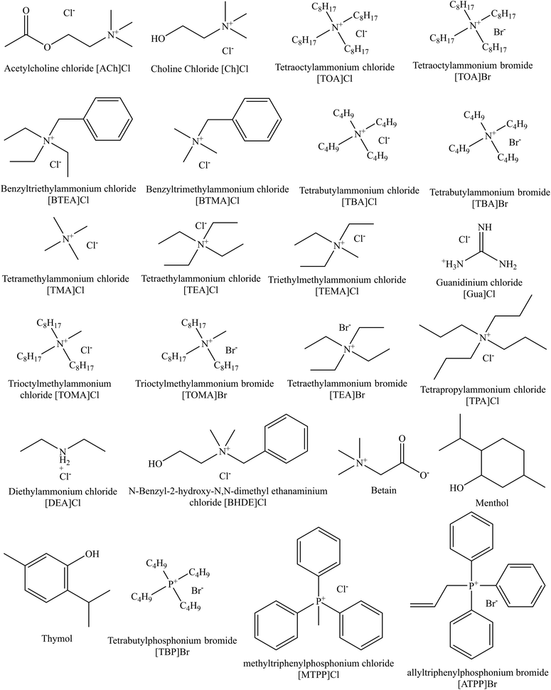
The COSMO-RS theory predicts thermodynamic properties by creating a virtual conductor around each molecule, where the surface area and screening charge density of each formed surface segment are calculated and based on this the σ-profiles are determined.55 As outlined in section 2.1, the COSMO files of investigated molecules were generated and used for thermodynamic property calculations. Examples of the 3D structures and COSMO cavities of modeled HBA and HBD molecules are presented in Fig. 3. Using the generated molecular surfaces shown in Fig. 3, the polarity distributions (σ-profiles) of the HBAs and HBDs were calculated using COSMOthermX.52 The σ-profile of a molecule is a probability distribution that quantifies the relative probability of a molecular surface segment having a certain screening charge density.56 As a result, the integrated area under the σ-profile curve may be used to obtain a description of the surface of a molecule, which is designated as Sσ-profiles. The Sσ-profiles molecular parameter is an a priori quantum chemistry parameter that characterizes the concentration and type of atoms within a certain σ-range. For more information on the Sσ-profiles molecular descriptor, details can be found in the work of Torrecilla et al. (2010).57
 |
| | Fig. 3 Representation of the ten Sσ-profile descriptors in the σ-range for the (a) HBA and (b) HBD of DESs along with their COSMO cavities. The σ-profile of each component is composed of 61 elements with a screening charge density range of −3 e nm−2 to +3 e nm−2. The molecular polarity is graphically represented by the colors blue and red, where blue is the negative screening charge density (i.e., “hydrogen bond donating capability”), and red is the positive screening charge density (i.e., “hydrogen bond accepting capability”). The green and yellow color regions characterize “neutral or nonpolar” molecular surfaces. | |
Fig. 3(a and b) displays the σ-profiles of HBAs and HBDs of DESs. It has been seen that the σ-profile distributions in hydrogen bond donor and acceptor regions as well as the σ-profile areas of the molecules vary widely, revealing a unique σ-profile property for each molecule.35 The σ-profiles are divided into three regions: H-bond acceptor (σ > 1 e nm−2), H-bond donor (σ < −1 e nm−2), and non-polar (−1 e nm−2 < σ > +1 e nm−2) regions. To determine the σ-profile input descriptors for the machine learning model, the σ-profiles of DES constituents were divided into 10 fractions (i.e., S1–S10) by integrating σ-profile px(σ) curves over the screening charge density, σ. As exemplified by HBA and HBD in Fig. 1a and b, the fractions of the Sσ-profiles are classified into five classes depending on the screening charge densities: (1) The strong donor region [S1 and S2], (2) the weak donor region [S3], (3) non-polar region [S4, S5, S6, and S7], (4) the weak acceptor region [S8], and (5) the strong acceptor region [S9 and S10].
The Sσ-profiles of the modeled DESs are defined as the molar-weighted average of the constituents, which is the standard approach used to define the DES in the literature.36,37 The equation is expressed as follows:
| |  | (3) |
where
xHBA and
xHBD are the mole fractions of HBA and HBD, respectively, while
Si,σ-profile is the descriptor in the
σ-profile region ‘
i’
i.e., from S1 to S10.
2.4. Development of the machine learning model
The concept of neural network models in the context of machine learning is inspired by the architecture of the cerebral cortex, which consists of neurons organized in layers and synapses between neurons of different layers. In an artificial neural network (ANN) model, the “neurons” are mathematical functions typically referred to as perceptrons whose output is binary, either 0 or 1, according to an activation function that toggles between these two outputs, based on input from other perceptrons. Similar to the biological counterpart, the perceptrons are organized in layers, with perceptrons of one layer receiving input from those of the preceding layer. The activated and deactivated perceptrons are collected in the last layer to create the necessary output response.58 ANNs have been successfully implemented across industries to solve a wide range of engineering problems, demonstrated exceptional performance in areas such as nonlinear function fitting and machine learning, and are well known for their high accuracy and robustness in solving complex problems.
Each perceptron has an associated weight that reflects how strongly it contributes to the ANN model's output. The following is a definition of the hidden neurons that are contained within the neural network (Hn,p):31
| |  | (4) |
where
Wn,p is the weight of the link between the input and the hidden layers,
n is the hidden layer
(1), and
p is the number of hidden neurons (9 neurons used in this work).
bn,p represents the intercept bias of the hidden neuron ‘
n’ of the hidden layer, and ‘
f’ is the activation or transfer function of the neuron.
In this work, an ANN-based machine learning model was developed using the JMP Pro statistical software (JMP SAS 14.3.0)59 by utilizing the temperature, pressure, and the 10 Sσ-profiles molecular descriptors as input features to predict the solubility of CO2 in DESs as an output variable. The predictive correlation is defined as follows:
| |  | (5) |
where

is the solubility of CO
2 in DES,
T and
P are the temperature (K) and pressure (kPa). The neural network toolbox of John's Macintosh Project statistical software (JMP Pro SAS 14.3.0) was used to design the fully connected multi-activation function neural network with a single layer. For ANN, 55% of the data was used for training, and 45% of the data was used for testing and the data were randomly split using the validation column maker in JMP Pro SAS 14.3.0. The network's learning rate was fixed to 0.1, the number of tours was set to 1000, and a squared penalty method was used for optimization. All other options in the JMP SAS 14.3.0 software were kept as default.
2.5. Model validation and performance
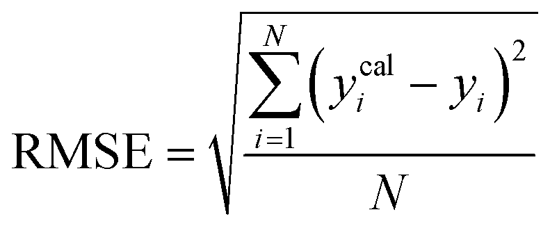
To assess the predictive capability of the developed machine learning model, different statistical parameters such as the determination coefficient (R2), average absolute relative deviation (AARD), mean absolute error (MAE), and root mean square error (RMSE) were calculated. R2 measures how accurately the model fits; the higher the R2 value, the better the model fits. The AARD, MAE, and RMSE values along with the following statistical parameter expressions, can be used to characterize the deviation between experimental and predicted CO2 solubility in DES.26,46| |  | (6) |
| |  | (7) |
| |  | (8) |
| |  | (9) |
where N is the total number of data points, yi and ȳm are the experimental CO2 solubility in DES and the average of the experimental data. ycali is the CO2 solubility computed by either the machine learning model or the COSMO-RS model.
3. Results and discussion
3.1. Solubility of CO2 in DES using the COSMO-RS model
The COSMO-RS model is an effective computational method for calculating thermodynamic properties and for screening solvents for gas solubilities. In many cases, only structural information of the solvent (i.e., here DES) and solute (i.e., here CO2) is typically required for COSMO-RS to calculate the solubility and other thermodynamic properties. In our earlier work on the dissolution of cellulose, hemicellulose, lignin, and plastic polymers, we demonstrated the usefulness of COSMO-RS and the results were validated against experimental data.54,56,60–62 In the literature, the COSMO-RS model has been extensively utilized for gas solubility predictions in a variety of solvents.25,63 Therefore, in the present study, we use the COSMO-RS model to calculate the solubility of CO2 in a variety of DESs.
To run COSMO-RS model for CO2 solubility, a large number of experimental data points were collected from the literature for CO2 solubility in 132 DESs over a wide range of temperatures (T = 293.15 K to 348.15 K), pressures (P = 26.3 kPa to 7620 kPa), and DES molar ratios (1:1 to 1:16). Similar experimental conditions (T, P, DESs, and molar ratios), were used as input to calculate the solubility of CO2 using COSMO-RS. The COSMO-RS predicted and experimental CO2 solubility data are compared and summarized in Fig. 4 and Table S1.† The COMSO-RS model calculates the solubility of CO2 in DESs with an AARD of 23.4% and R2 of 0.85. Table S1† shows that the calculated solubility of CO2 increases with pressure and decreases with increasing temperature, which is in agreement with experimental observations. However, because of the relatively high AARD values, COSMO-RS agreement with experiment is only qualitative, not quantitative. For example, the experimental solubility of CO2 (ln(xCO2)) in [Ch]Cl-phenol DES at 1:2 molar ratio is −4.87 at T = 293.15 K and P = 197.2 kPa, and −4.95 at T = 303.15 K and P = 198.2 kPa. The corresponding COSMO-RS predicted ln(xCO2) are −3.46 and −3.71, respectively, results within ∼25–28% of AARD, indicating that COSMO-RS correctly predicts the CO2 solubility qualitatively (as the T increases, ln(xCO2) decreases). It is worth noting that the AARD between experimental and COSMO-RS predictions decreases with increasing temperature. For instance, the AARD of [TBA]Cl-LA at 1:2 decreases with increasing temperatures (AARD at 93 kPa for 308 K and 318 K are 11.3% and 6.8%, respectively). In contrast, the AARD increases with pressure (e.g., [TBA]Cl-LA (1:2) DES, AARD is 11.3% to 19.5% for 93 kPa to 1992 kPa at 308 K). The higher AARD at lower temperatures may be because the COSMO-RS model underpredicts the CO2 solubility in DESs, and also might be a possibility for higher viscosity of DESs which limits the solubility.
 |
| | Fig. 4 Correlation between the COSMO-RS predicted and experimental CO2 solubility in deep eutectic solvents. | |
A closer look at Fig. 4 shows that the COSMO-RS-calculated CO2 solubility values are lower than the experimental results. Interestingly, at higher temperatures, the AARD values are lower than at lower temperatures and the DESs with longer alkyl chain length HBAs (e.g., [TBA]+) or larger size (e.g., [ATPP]+ cations/salts) with phenols as HBD show AARDs less than 10%, which is in excellent agreement with experimental solubility.
We also compared our COSMO-RS-calculated results with related works in the literature. Recently, Liu et al. (2020)25 used the COSMO-RS model to calculate the solubility of CO2 in 35 DESs with 502 data points. They reported that the average ARD between experimental and COSMO-RS predictions was 59.2–78.2%, which is a much higher deviation than current study predictions. This may be due to not using the energetically optimal DESs (HBA and HBD) conformers in their COSMO-RS calculations, resulting in higher CO2 solubility deviations. However, with increasing pressure and decreasing temperature, the discrepancies in the present work become larger, and this is consistent with the observations by Liu et al. (2020)25 and Kamgar et al. (2017).64 Therefore, using optimal molecular conformers of DESs provides a significant benefit to COSMO-RS calculations, which in turn leads to better predictions of CO2 solubility.
3.2. Development of multilinear regression model
Since a large deviation was observed between the COSMO-RS predicted and experimental CO2 solubilities, we searched for a systematic correction of COSMO-RS predictions to boost the model performance for predicting CO2 solubility in DESs. In recent studies, Liu et al. (2018)65 corrected the COSMO-RS-based predictions for CO2 solubility in ionic liquids and obtained a good agreement between experimental and predicted results after model correction with T, P, and molar ratio (r). Another study by Liu et al. (2020)25 reported corrected COSMO-RS predictions for CO2 solubility in DESs and observed a better correlation between experimental and predicted results after correction. We used a multilinear regression (MLR) model developed by Liu et al. (2020) to calculate the CO2 solubility; however, the average deviation was significantly higher (59%) than our original COSMO-RS predicted results. Therefore, we developed a separate multilinear regression (MLR) model by incorporating the original COSMO-RS calculated CO2 solubilities, DES molar ratios, temperature, and pressure-dependent parameters. The following multilinear regression model was devised:| |  | (10) |
Here, r, T, and P are the molar ratio of DES, temperature (K), and pressure (kPa). k1–k6 are the fitting parameters. To obtain the k1–k6 parameters, the experimental results of CO2 solubilities in DESs at different molar ratios, temperatures, and pressures were used as fitting targets. In total 1973 experimental data points were included in fitting with a multilinear regression model. The values of the fitting parameters are listed in Table 1.
Table 1 Adjustable parameters of eqn (10)
| Adjustable parameters |
|
k
1
|
k
2
|
k
3
|
k
4
|
k
5
|
k
6
|
| 332.37 |
−1799.04 |
7.1 × 10⁻⁵ |
−4.13 × 10⁻⁵ |
−1.116 |
4.92 |
The CO2 solubilities obtained with the MLR model were compared with the corresponding experimental solubilities (Fig. 5). The MLR model results are much closer to the experimental CO2 solubilities  than the original COSMO-RS model, with an AARD of 12%, and R2 of 0.87. Further, the results of the MLR model developed in the present study were compared with those of the MLR model of Liu et al. (2020),25 and we found that the MLR model in the present study yields lower AARD values (12%) than that of Liu et al. (2020) (59%). A higher deviation was also reported by Liu et al. (2021)63 during their study on the evaluation of MLR model proposed by Liu et al. (2020)25 in predicting the CO2 solubility in a new set of DESs and molar ratios. It is important to mention that Liu et al. (2020)25 developed a model that has certain limitations, such as not being applicable to situations with higher molar ratios of HBA to HBD (≥1:7), new DESs, and higher pressures (≥3000 kPa). Moreover, the model was developed with a smaller set of data points (502) and a smaller number of DESs (35); thus, it cannot be considered as a universal model for CO2 solubility prediction in all situations. In contrast, the MLR model of the present study was developed by considering a wider range of HBA to HBD molar ratios (1:1 to 1:16), temperatures (293.15 K to 348.15 K), and pressures (26.3 kPa to 7620 kPa) than that of the study by Liu et al. (2020), as well as a larger set of experimental data points (i.e., 1973), and a greater diversity of different DESs (132).
 |
| | Fig. 5 Correlation between the COSMO-RS corrected multilinear regression model and experimental CO2 solubility in deep eutectic solvents. | |
3.3. Development of machine learning model for CO2 solubility
As well as the MLR, a machine learning model that is based on an artificial neural network (ANN) has been developed that is even more accurate and reliable for predicting CO2 solubility. The input features for the machine learning model are COSMO-RS-calculated Sigma profile descriptors (Sσ-profiles-1 to Sσ-profiles-10), temperature, and pressures. We calculate a binned probability of polarized charge at the molecular surface (i.e., the COSMO-RS-derived Sigma profile) that we hypothesized is likely to implicitly capture the propensity for certain intermolecular interactions, either among DES molecules or between DES molecules and CO2. This hypothesis will be validated through the ML model's performance as well as the post hoc interrogation of the ML model to ascertain the relative importance of features used to train the model.
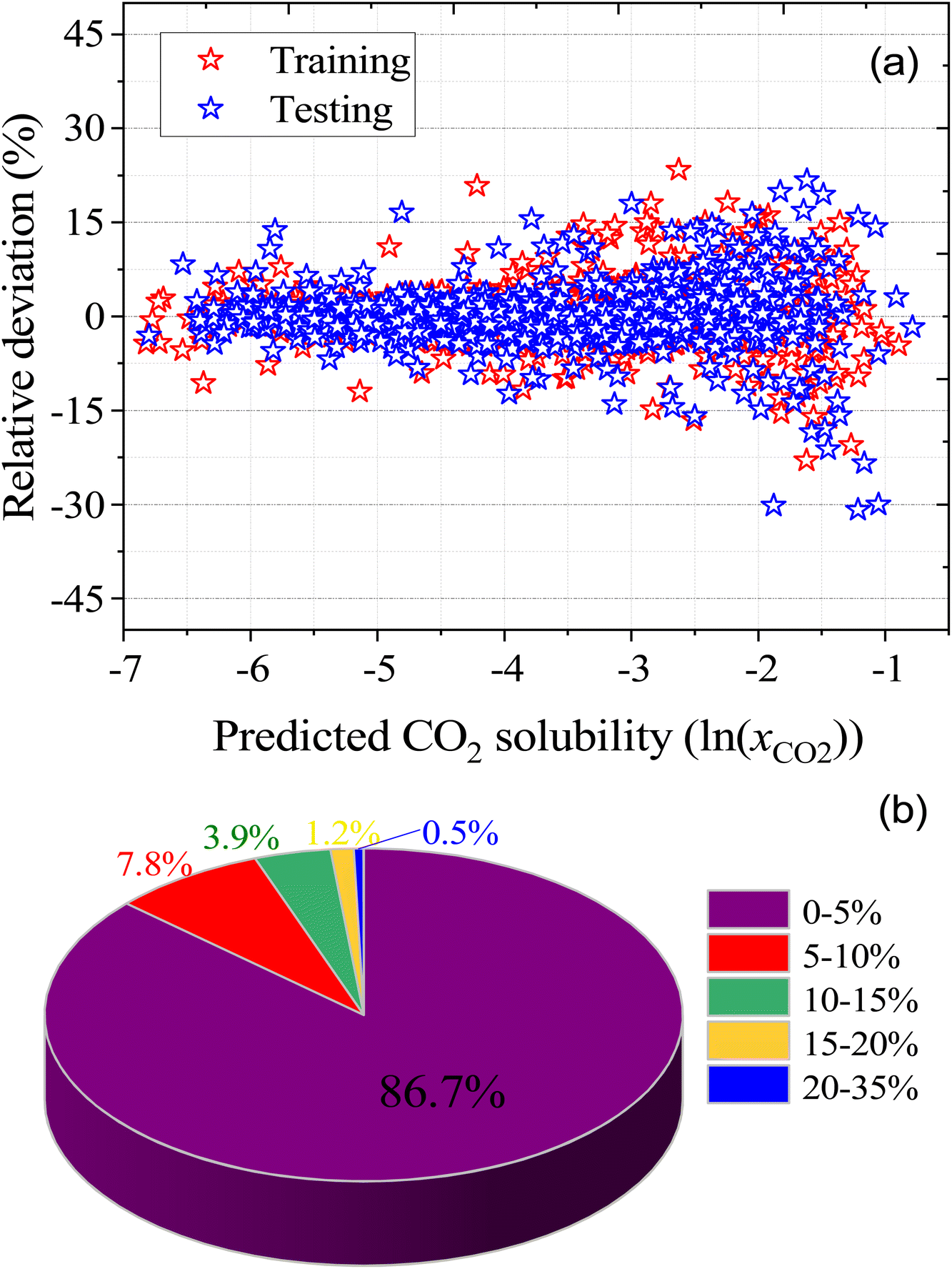
For ML, 55% (1084 data points) of the data was used for training and the remaining 45% (889 data points) of the data was used for testing. Fig. 6 illustrates the correlation of experimental and ML predicted CO2 solubilities in the training and testing sets. Fig. 6 also lists the statistical parameters for the ML model including R2, AARD, MAE, and RMSE. As depicted in the parity plot in Fig. 6, the predictions for the training and testing sets are in excellent agreement with experimental data. For the total set of data points, R2, AARD, MAE, and RMSE values are 0.99, 2.72%, 0.087, and 0.1287, respectively, which are all at a very desirable level of accuracy. Furthermore, statistical residual analysis was also performed for the ML model and confirmed the goodness-of-fit through a normal probability plot of the relative deviations, relative deviations vs. predicted values plot, and histogram of the relative deviations. Fig. S1 and S2† depict the statistical analysis plots and show that the CO2 solubility relative deviations are within 10% with an AARD of 2.72% and RMSE of 0.1287. Moreover, the distribution of the relative deviations in different ARD ranges is also shown in Fig. 7; the majority of CO2 solubility prediction data (87%) lies within 5% of AARD and 94.5% of data within 10% of AARD. Only 1.7% of the data lies beyond 15% of AARD. These results clearly demonstrate the accuracy of the developed ML model for CO2 solubility predictions. However, the ML model has certain limitations; the model predictions are more accurate for physical-based DES systems, but not reliable for chemical-based DESs.
 |
| | Fig. 6 Experimental and predicted CO2 solubility in DESs using an ANN-based machine learning model (a) training set and (b) testing set. | |
 |
| | Fig. 7 (a) relative deviation between the experimental and predicted CO2 solubilities in DES, and (b) the distribution of the absolute relative deviation in different deviation ranges. | |
3.4. Applicability domain and covariance matrix
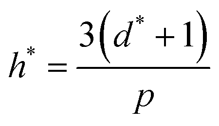
High uncertainty in experimental data leads to a less accurate ML model, particularly if there are systematic – as opposed to random – errors in the data. Nevertheless, accurate experimental data with explicitly low uncertainty (and data where uncertainties in the measurements, such as error bars, are reported) is scarce, and to some extent, investigators seeking to develop predictive models using supervised ML must contend with this. To mitigate this problem and assess for the presence of outliers that might confound our model accuracy, we performed the applicability domain (AD) analysis. The applicability domain (AD) is a key concept in ML as it enables the evaluation of the uncertainty in a prediction for a given target based on its similarity to the data points used in the training set. AD has been extensively utilized in ML models to identify structural outliers and establish a prediction accuracy range for a given set of molecules.66 The AD can be calculated using a variety of methods; however, the most prevalent is the leverage approach, in which the model is tested based on the leverage value (hi) for each chemical. Lower hi values (hi< h*) indicate higher similarity to the training set. In contrast, molecules with higher hi values than the critical leverage (hi > h*) represent molecules that are “different” from the molecules in the training set, and their prediction may be less reliable owing to the higher degree of extrapolation. The leverage value is defined as follows.66where νi is a matrix with dimensions 1 × d* containing input parameters, d* denotes the number of input variables in machine learning model, V is a p × d* matrix where p denotes the number of experimental data points in training sets, and the superscript T represents the transpose of the matrices. The crucial leverage value (h*) is determined using the formula below:66| |  | (12) |
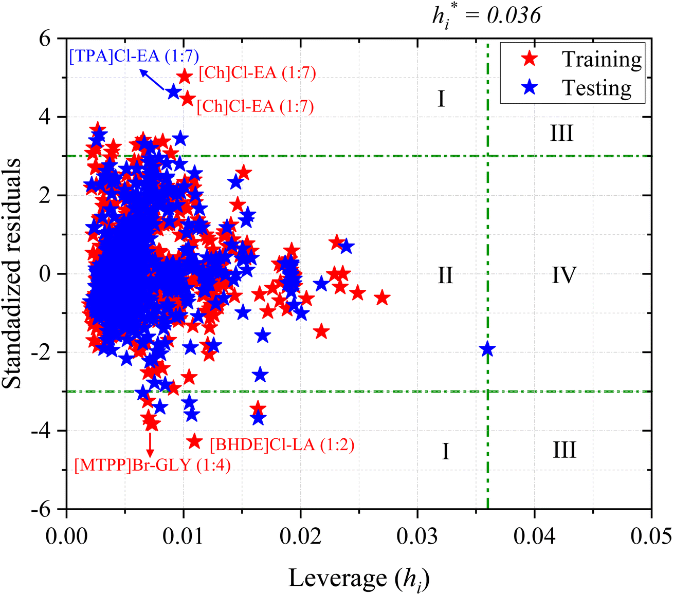
A William plot illustrates a model's domain of applicability by plotting the standardized residuals (SDR) versus the leverage values (hi) of each data point. The SDR boundaries in the William plot are between −3 < SDR < +3 and 0 < hi < h*.67
Fig. 8 shows the Williams plot for each data point, where the AD boundaries consist of a critical leverage h* = 0.036 (vertical green dashed line) and the SDR, which are ±3 (two horizontal green dashed lines). The boundary lines divide the Williams plot into four major regions (I, II, III, and IV). Predictions of the chemical substances in region I are biased, which is maybe due to the large uncertainty in the experimental data rather than wrong model predictions. The data points in region II are within the application domain of the model and these predictions are considered reliable. Interpolation among the corresponding data points can be done with reduced uncertainty. The chemical substances in region III are both response outliers (high SDR) and high leverage (>h*) values. If the data points are slightly higher than critical leverage h* and SDR, the impact on the model is negligible. However, if the data points are far away from critical leverage h* and SDR, the outlier should be removed from the model's scope of application. Finally, the data points in region IV are both response outliers and high leverage values (i.e., >h*), indicate that the predictions have a certain deviation.
 |
| | Fig. 8 Williams plot (standardized residual vs. leverage) of the total set of ML model for the CO2 solubility in DESs. | |
From Fig. 8, the ANN model exhibits no structural outliers in region IV as all the data points have leverage values lower than the critical value (hi < h*; region II). However, the predictions of CO2 solubility in a few DESs in both the training and testing sets are considered structural outliers as they exhibit SDR values greater than three limits (±3; region I), which brings down the AD coverage to 98.22%. 35 data points are outside of the AD limit (region I and IV), accounting for 1.78% of the total (1973), and the double extraterritorial region is blank (region III). The response outliers in the ANN model include [Ch]Cl-EA (1:7), [TPA]Cl-EA (1:7), [BHDE]Cl-LA (1:2), [ATPP]Br-DEG (1:4 and 1:10), [ATPP]Br-TEG (1:4), and [MTPP]Br-GLY (1:4). The response outliers above the SDR ± 3 boundaries may arise from large deviations in experimental measurements, and are mostly at lower temperatures and pressures (<400 kPa) in both the training and testing sets. Based on the obtained AD analysis, it can be concluded that the prediction of a new combination of DES that (i) are within the model's applicability domain and (ii) contain similar constituents to the ones utilized in the training set could be considered reliable. However, the development of new DESs that are not within the model's applicability domain should be treated with more caution. In addition, it may be worthwhile to perform experiments carefully and precisely at lower temperatures and pressures. Overall, the AD results indicate that the developed ML model possesses ample robustness and generalizability due to its large AD and structural coverage.
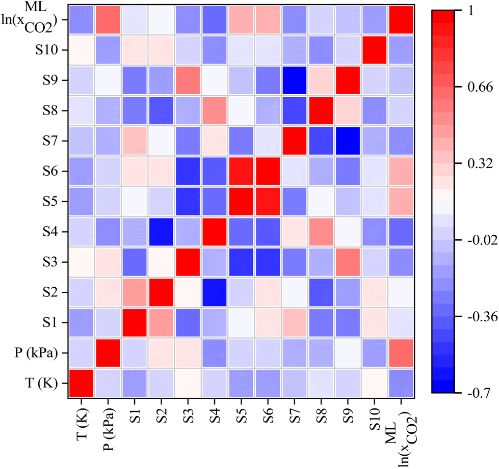
In addition, the covariance matrix plot between ML input features was investigated and depicted in Fig. 9. From Fig. 9, there is no significant linear connection between input features of ML except Sσ-profiles-5 (S5) and Sσ-profiles-6 (S6) of Sigma profile descriptors. The lack of linear correlation between input features indicates that the features are nonredundant and may result in a more robust ML model that more accurately predicts CO2 solubility. Fig. 9 also illustrates the correlation between ML input features and predicted CO2 solubility. The positive influence of the input features on the CO2 solubility prediction is indicated by the positive covariance matrix value, while the negative covariance matrix value indicates negative influence. It is worth mentioning that pressure, S5, S6, S2, S1, and S9 show a positive influence on the CO2 solubility predictions, implying that as the value of these parameters increases, the solubility of CO2 is seen to increase. On the other hand, the temperature has shown a negative correlation with CO2 solubility, which implies that CO2 solubility decreases with an increase in temperature; this result is in accordance with the experimental observations.
 |
| | Fig. 9 Heatmap of the covariance matrix. Correlation between features of the input descriptor set and predicted CO2 solubility in DESs. | |
3.5. Reliability and rationality of developed ML model and comparison with literature reported models
To further evaluate the reliability of the ML model developed in this work, the effect of input variables such as temperature, pressure, molar ratio, and HBA/HBD on the CO2 solubility predictions was investigated and compared to experimental measurements. Fig. 10a and S3a† show the predicted solubility of CO2 in DESs over a wide range of temperatures (290.15 K to 330.15 K) for [Ch]Cl-Guaiacol (1:4) and [ATPP]Br-TEG (1:10) as an example DES. The solubility of CO2 decreases significantly with increasing temperature. Fig. 10(a–c) shows the effect of pressure on the solubility of CO2 in different DESs at constant temperature. The solubility of CO2 increases linearly with pressure and agrees well with the experimental observations. Further, the effects of molar ratios and HBA/HBD were also examined, and the results are depicted in Fig. 10(c and d) and Fig. S3b.† It has been observed that for DESs with the same HBA at a similar molar ratio, the longer the alkyl chain length of the HBD, the higher the solubility of CO2. For example, for the DES [ATPP]Br with TEG (triethylene glycol) or DEG (diethylene glycol) at 1:10 or 1:16 molar ratio, [ATPP]Br:TEG shows higher solubility of CO2 than [ATPP]Br:DEG. This is due to the larger free volume and stronger van der Waal (vdW) interactions of TEG with CO2.33 The same trend was also noticed for the HBAs, where if alkyl chain length of HBA increases, the solubility of CO2 tends to increase. For instance, the predicted CO2 solubility in [TBA]Br:hexanoic acid (1:4) and [TEA]Br:hexanoic acid (1:4) can be compared under similar conditions (T = 303.15 K and P = ∼1030 kPa). [TBA]Br:hexanoic acid (1:4) achieves higher CO2 solubility than [TEA]Br:hexanoic acid (1:4), due to its stronger intermolecular interactions with CO2. Moreover, as the molar ratio of HBA to HBD increases from 1:10 to 1:16 for [ATPP]Br:TEG/DEG DESs, the solubility of CO2 decreases, which is again in line with the experimental measurements.68Fig. 10 demonstrates the rationality and reliability of ML model to predict these aforementioned trends.
 |
| | Fig. 10 ANN-based machine learning predicted CO2 solubilities in (a) [Ch]Cl-Guaiacol (1:4) at different temperatures, (b) [Ch]Cl and [ATTP]Br-based DES at different pressures, and (c and d) effect of molar ratio, HBDs and HBAs on CO2 solubility. | |
The developed ML model shows an excellent performance and rationality in predicting CO2 solubility and reproducing experimentally observed trends in the solubility that vary systematically with physicochemical characteristics of the solvent. It is also of interest to compare the model performance with that of other computational models reported in the literature. Table 2 shows the comparison of the results of the different models along with their AARD values. From Table 2, traditional thermodynamic models such as PR-EoS (Peng-Robinson Equation of State) and PC-SAFT show good performance with low AARDs. However, a caveat is that a very small set of data points and DESs was used in validating these models. Also, these models require experimental input data to fit molecule-specific binary interaction and mixing parameters, which restricts their applicability to new solvent systems such as ILs and DESs. Considering the inapplicability of the traditional models for novel solvent systems (i.e., DES-CO2), the development of machine learning or QSPR models are emerging. Recently, Wang et al. (2021)26 proposed a QSPR model based on random forest regression for CO2 solubilities in DESs and reported an AARD of 7.76%, which is three times higher than that of the model in the present study (AARD is 2.74%). On the other hand, it is important to note that a greater number of DESs and data points were used to develop our model than that of Wang et al. (2021).26
Table 2 Comparison of developed CO2 solubility predicted models (QSPR and traditional thermodynamic models as well as equations of state methods)
| Model |
No. of DESs (molar ratio HBA:HBD) |
Data points |
T (K) |
P (kPa) |
AARD (%) |
Ref. |
| PC-SAFT |
4 (2:1 to 3:1) |
180 |
298.15–318.15 |
10–2000 |
3.97% |
Zubeir et al. (2016)28 |
| PR-EoS |
3 (1:2) |
57 |
309–329 K |
40–160 |
0.80% |
Mirza et al. (2015)71 |
| COSMO-RS |
35 (1:2 to 1:6) |
502 |
293.15–333.15 |
71.5–2068 |
78.2% |
Liu et al. (2020)25 |
| COSMO-RS-based MLR |
35 (1:2 to 1:6) |
502 |
293.15–333.15 |
71.5–2068 |
10.8% |
Liu et al. (2020)25 |
| COSMO-RS |
59 (1:1.5 to 1:16) |
1011 |
293.15–343.15 |
36–12730 |
64.81% |
Wang et al. (2021)26 |
| QSPR (random forest regression) |
59 (1:1.5 to 1:16) |
1011 |
293.15–343.15 |
36–12730 |
7.76% |
Wang et al. (2021)26 |
| CPA |
13 (1:2 to 1:6) |
353 |
293.15–343.15 |
63–11820 |
7.02% |
Pelaquim et al. (2022)30 |
| PR-EoS |
13 (1:2 to 1:6) |
353 |
293.15–343.15 |
63–11820 |
5.50% |
Pelaquim et al. (2022)30 |
| COSMO-RS |
132 (1:1 to 1:16) |
1973 |
293.15–343.15 |
26.3–7620 |
23.4% |
Present study |
| COSMO-RS-based MLR |
132 (1:1 to 1:16) |
1973 |
293.15–343.15 |
26.3–7620 |
12% |
Present study |
| Machine learning (ANN) |
132 (1:1 to 1:16) |
1973 |
293.15–343.15 |
26.3–7620 |
2.72% |
Present study |
On the other hand, the COSMO-RS model is widely used to predict the solubility of CO2 in a variety of solvent systems (molecular solvents, ionic liquids, and DESs), so it is instructive to compare the accuracies of that model reported in the literature with those of our ML model derived from COSMO-RS features that is presented here, as well as the corresponding accuracies of our in-house prediction using just the COSMO-RS model itself without ML. As summarized in Table 2, the AARD of COSMO-RS-predicted CO2 solubilities reported in the literature are in the range of 65–78.2%, while in our case, it is 23.4%. The lower AARD yielded by the COSMO-RS model in the present study is due to the consideration of multiple lowest energy molecular conformers of HBA and HBD, leading to more reliable predictions of CO2 solubility. Further, Liu et al. (2020)25 have developed a MLR model for CO2 solubility and reported 10.8% of AARD, which is consistent with our COSMO-RS-based MLR model predictions. However, the ML model is more reliable and accurate for CO2 solubility prediction than the COSMO-RS model, but nonetheless the COSMO-RS-derived descriptors are useful for developing ML models.
3.6. Development of new DESs for improving CO2 solubility
After the successful development of a ML model and the careful evaluation of CO2 solubility prediction in 132 different DESs, the ML model can now be used to predict the solubility of CO2 in new combinations of DESs whose CO2 solubilities have not been reported in the literature. The importance of input features was calculated using the Shapley additive explanations (SHAP) method, which provides a unified approach for interpreting output of machine learning methods and provide a guide to design of novel DES for carbon capture from a structural perspective. Lundberg and Lee (2017)69 developed SHAP to elucidate the ML predictions in terms of the training features based on game theory. An advantage of the SHAP method is that it can be used to interpret the feature importance for models that have traditionally been deemed to be uninterpretable, or ‘black-box’, including models such as neural networks.70 As shown in Fig. 11, the SHAP analysis ranks the features in terms of their importance, while the SHAP value indicates how varying a certain feature is likely to affect the CO2 solubility. A positive SHAP value for a feature suggests an increase in CO2 solubility with increasing value of the feature, while a negative SHAP value implies the reverse. Pressure, S5, S9, S8, and S7 are thus found to be particularly important in the prediction of CO2 solubility. From a structural perspective, the DESs with higher values of S4, S5, and S6 (non-polar region), indicating that a molecule possessing larger free volumes and stronger van der Waal (vdW) interactions, result in higher solubilities of CO2. This is supported by previous work that suggested that molecules with these attributes show higher CO2 solubility. In addition, the lower values of the DESs polar regions (S1, S2, S3, S8, S9, and S10), implies that the cross interaction between DES molecules will be weaker and leads to stronger interaction with CO2. The SHAP feature importance analysis also correctly captures the temperature and pressure effect on the CO2 solubility (Fig. 11); as the temperature increases, CO2 solubility decreases, and CO2 solubility increases with increasing pressure.
 |
| | Fig. 11 SHAP feature importance for the testing data set of CO2 solubility in deep eutectic solvents. | |
Based on the SHAP analysis, HBAs such as [TBA]Br, [TBP]Br, [TOA]Br, [ATPP]Br, menthol, and thymol, and HBDs such as TEG, DEG, decanoic acid (DecA), methyldiethanolamine (MDEA), ethanolamine (EA), ethylenecyanohydrin (ECH), and EG are potential candidates for high CO2 solubility due to the higher values of S4, S5, and S6 and lower values of polar regions (S1–S3 and S8–S10). It has also been reported that longer alkyl chain lengths of DESs, or hydrophobic moieties in general, are better solvents for CO2.23,33 Bearing this in mind, novel DES combinations were chosen based on our ML predictions and the following DESs combinations are proposed at different molar ratios and a wide range of pressures: menthol–decanoic acid (1:2), menthol–dodecanoic acid (1:2), [TBP]Br-TEG, [TOA]Br-TEG, [TOMA]Br-TEG, [ATPP]Br-DECA, [ATPP]Br-EA, [ATPP]Br-MDEA, and [ATPP]Br-ECH. Fig. 12 shows the calculated solubility of CO2 in the newly proposed DESs at 298.15 K and different pressures. As the pressure increases, the solubility of CO2 predicted by the ML model also increases, in accord with Henry's Law. More importantly from the perspective of solvents for CO2 capture, menthol–DecA, [TBA]Br-TEG, [TOMA]Br-TEG, and [ATPP]Br-DecA appear to be promising solvents for improving CO2 solubilities. The higher solubility in menthol- and phosphonium-based DESs is due to larger free volumes of HBA and HBD and strong interactions with CO2 through vdW interactions.23,68 Furthermore, to confirm the molar ratios of newly developed DES combinations, we performed COSMO-RS for menthol and decanoic acid/dodecanoic acid as an example of calculating the eutectic point composition. The eutectic point compositions for [ATPP]Br-based DES were not calculated and validated due to the lack of phase transition properties (i.e., melting point and heat fusion values) in the literature. The detailed procedure for the calculation of the eutectic point composition is discussed in our previous study.19 Fig. S4† shows the COSMO-RS-calculated eutectic point composition of both DESs (menthol: DECA and menthol: DoDECA). Menthol forms a eutectic point with decanoic acid and dodecanoic acids, and the calculated eutectic point is in liquid state at room temperature. Moreover, menthol–decanoic acid DES has a lower eutectic temperature (TE = 265.8 K) than menthol–dodecanoic acid (TE = 279 K), which indicates that menthol–DECA has a lower viscosity than menthol–DoDECA due to the larger liquid window.
 |
| | Fig. 12 Development of new DESs combination for improving CO2 solubilities using the machine learning model, DES composed of (a) menthol as HBA and decanoic acid and dodecanoic acid as HBDs, (b) [ATTP]Br HBA and EA, DECA, MDEA, and ECH are HBDs, and (c) [TBP]Br, [TOA]Br, and [TOMA]Br are HBAs with TEG HBD. | |
4. Conclusions
In the present work, an accurate method for predicting CO2 solubility in DES has been developed. We established a database containing 1973 experimental data points for CO2 solubility in 132 DESs at different temperatures and pressures. The database was used for verification and development of COSMO-RS models and ML models. The AARD between COSMO-RS calculated and experimental CO2 solubilities was relatively high i.e., 23.4%. However, the COSMO-RS predicted CO2 solubility data was corrected using a multilinear regression (MLR) model with six adjustable universal parameters that reduced the AARD to 12%. Further improvement of performance was obtained with a machine learning model using the COSMO-RS-derived molecular descriptors such as the Sigma profile as input features for the prediction of CO2 solubility in 132 different DESs at various temperatures, pressures, and molar ratios. The developed ML model has excellent predictive performance with high R2 (0.99) and low AARD (2.72%) and MAE (0.087) values and also can be used to interpret the influences of input variables. The presented results suggest that the σ-profiles are useful molecular descriptors of DES, given that our model trained on those features gave excellent performance. In comparison with models reported in the literature, the ML model developed here more accurately predicts CO2 solubilities in DESs and can therefore be a useful tool for designing and selecting a DESs for CO2 capture.
Conflicts of interest
The authors declare no competing financial interest.
Author contributions
M. M.: conceptualization, project design, data curation, performed the COSMO-RS calculations, developed ML models (ANN and MLR), and wrote the manuscript. O. D.: helped in the development of ML models and reviewed the manuscript. B. A. S., J. C. S., M. K. K, and S. S.: obtained the project grants, supervision, and reviewed the manuscript.
Acknowledgements
This work was part of the DOE Joint BioEnergy Institute (https://www.jbei.org) supported by the U. S. Department of Energy, Office of Science, Office of Biological and Environmental Research, through contract DE-AC02-05CH11231 between Lawrence Berkeley National Laboratory and the U. S. Department of Energy. Support was also provided by the US Department of Energy (DOE), Office of Science, through the Genomic Science Program, Office of Biological and Environmental Research (contract no. FWP ERKP752). Seema Singh and Michelle K. Kidder also acknowledged the U. S. Department of Energy, Office of Science, Office of Basic Energy Sciences, Division of Chemical Sciences, Geosciences, and Biosciences (CSGB) Grant Number DE-SC0022273 and 3ERKCG25 respectively, for partially supporting this research. The United States Government retains and the publisher, by accepting the article for publication, acknowledges that the United States Government retains a non-exclusive, paid-up, irrevocable, world-wide license to publish or reproduce the published form of this manuscript, or allow others to do so, for United States Government purposes.
References
- K. A. Pishro, G. Murshid, F. S. Mjalli and J. Naser, Chin. J. Chem. Eng., 2020, 28, 2848–2856 CrossRef CAS.
- P. Cianconi, S. Betrò and L. Janiri, Front. Mol. Psychiatry, 2020, 11, 74 CrossRef PubMed.
- J. Jiang, B. Ye and J. Liu, Appl. Energy, 2019, 235, 186–203 CrossRef CAS.
- G. Li, D. Deng, Y. Chen, H. Shan and N. Ai, J. Chem. Thermodyn., 2014, 75, 58–62 CrossRef CAS.
- F. P. Pelaquim, A. M. Barbosa Neto, I. A. L. Dalmolin and M. C. d. Costa, Ind. Eng. Chem. Res., 2021, 60, 8607–8620 CrossRef CAS.
-
B. Metz, O. Davidson, H. d. Coninck, M. Loos and L. Meyer, Working Group III of the Intergovernmental Panel on Climate Change. IPCC Special Report on Carbon Dioxide Capture and Storage, Cambridge University Press, 2005 Search PubMed.
- W. Gao, S. Liang, R. Wang, Q. Jiang, Y. Zhang, Q. Zheng, B. Xie, C. Y. Toe, X. Zhu and J. Wang, Chem. Soc. Rev., 2020, 49, 8584–8686 RSC.
- Global CO2 Emissions Researched an All-Time High of 36.3 gigatons in 2021, https://www.iea.org/reports/global-energy-review-co2-emissions-in-2021-2, (accessed September 21, 2022, 2022).
- Y. Chen and T. Mu, Green Chem., 2019, 21, 2544–2574 RSC.
- A. Dubey and A. Arora, J. Cleaner Prod., 2022, 133932 CrossRef CAS.
- L. Riboldi and O. Bolland, Int. J. Hydrogen Energy, 2016, 41, 10646–10660 CrossRef CAS.
- X. Zhang, X. Zhang, H. Dong, Z. Zhao, S. Zhang and Y. Huang, Energy Environ. Sci., 2012, 5, 6668–6681 RSC.
- F. Yan, N. R. Dhumal and H. J. Kim, Phys. Chem. Chem. Phys., 2017, 19, 1361–1368 RSC.
- P. Tamilarasan and S. Ramaprabhu, J. Mater. Chem. A, 2015, 3, 101–108 RSC.
- P. Prakash and A. Venkatnathan, RSC Adv., 2016, 6, 55438–55443 RSC.
- E. L. Smith, A. P. Abbott and K. S. Ryder, Chem. Rev., 2014, 114, 11060–11082 CrossRef CAS PubMed.
- B. B. Hansen, S. Spittle, B. Chen, D. Poe, Y. Zhang, J. M. Klein, A. Horton, L. Adhikari, T. Zelovich and B. W. Doherty, Chem. Rev., 2021, 121, 1232–1285 CrossRef CAS PubMed.
- R. Verma, M. Mohan, V. V. Goud and T. Banerjee, ACS Sustainable Chem. Eng., 2018, 6, 16920–16932 CrossRef CAS.
- M. Mohan, K. Huang, V. R. Pidatala, B. A. Simmons, S. Singh, K. L. Sale and J. M. Gladden, Green Chem., 2022, 24, 1165–1176 RSC.
- P. K. Naik, M. Mohan, T. Banerjee, S. Paul and V. V. Goud, J. Phys. Chem. B, 2018, 122, 4006–4015 CrossRef CAS.
- M. Mohan, P. K. Naik, T. Banerjee, V. V. Goud and S. Paul, Fluid Phase Equilib., 2017, 448, 168–177 CrossRef CAS.
- Y. Chen, N. Ai, G. Li, H. Shan, Y. Cui and D. Deng, J. Chem. Eng. Data, 2014, 59, 1247–1253 CrossRef CAS.
- A. Alhadid, J. Safarov, L. Mokrushina, K. Müller and M. Minceva, Front. Chem., 2022, 300 Search PubMed.
- X. Liu, B. Gao, Y. Jiang, N. Ai and D. Deng, J. Chem. Eng. Data, 2017, 62, 1448–1455 CrossRef CAS.
- Y. Liu, H. Yu, Y. Sun, S. Zeng, X. Zhang, Y. Nie, S. Zhang and X. Ji, Front. Chem., 2020, 8, 82 CrossRef PubMed.
- J. Wang, Z. Song, L. Chen, T. Xu, L. Deng and Z. Qi, Green Chem. Eng., 2021, 2, 431–440 CrossRef.
- R. Haghbakhsh and S. Raeissi, J. Mol. Liq., 2018, 250, 259–268 CrossRef CAS.
- L. F. Zubeir, C. Held, G. Sadowski and M. C. Kroon, J. Phys. Chem. B, 2016, 120, 2300–2310 CrossRef CAS.
- E. A. Crespo, L. P. Silva, J. O. Lloret, P. J. Carvalho, L. F. Vega, F. Llovell and J. A. Coutinho, Phys. Chem. Chem. Phys., 2019, 21, 15046–15061 RSC.
- F. P. Pelaquim, R. G. Bitencourt, A. M. B. Neto, I. A. L. Dalmolin and M. C. da Costa, Process Saf. Environ. Prot., 2022, 163, 14–26 CrossRef CAS.
- L. F. Zubeir, D. J. Van Osch, M. A. Rocha, F. Banat and M. C. Kroon, J. Chem. Eng. Data, 2018, 63, 913–919 CrossRef CAS.
- R. Biswas, J. Mol. Model., 2022, 28, 1–8 CrossRef PubMed.
- J. Wang, H. Cheng, Z. Song, L. Chen, L. Deng and Z. Qi, Ind. Eng. Chem. Res., 2019, 58, 17514–17523 CrossRef CAS.
- H. S. Salehi, R. Hens, O. A. Moultos and T. J. Vlugt, J. Mol. Liq., 2020, 316, 113729 CrossRef CAS.
- D. O. Abranches, Y. Zhang, E. J. Maginn and Y. J. Colón, Chem. Commun., 2022, 58, 5630–5633 RSC.
- T. Lemaoui, A. S. Darwish, A. Attoui, F. A. Hatab, N. E. H. Hammoudi, Y. Benguerba, L. F. Vega and I. M. Alnashef, Green Chem., 2020, 22, 8511–8530 RSC.
- T. Lemaoui, A. Boublia, A. S. Darwish, M. Alam, S. Park, B.-H. Jeon, F. Banat, Y. Benguerba and I. M. AlNashef, ACS Omega, 2022, 7, 32194–32207 CrossRef CAS PubMed.
- A. Boublia, T. Lemaoui, F. A. Hatab, A. S. Darwish, F. Banat, Y. Benguerba and I. M. AlNashef, J. Mol. Liq., 2022, 366, 120225 CrossRef CAS.
- O. Nordness, P. Kelkar, Y. Lyu, M. Baldea, M. A. Stadtherr and J. F. Brennecke, J. Mol. Liq., 2021, 334, 116019 CrossRef CAS.
- M. Khandelwal and T. Singh, Int. J. Rock Mech. Min. Sci., 2009, 46, 1214–1222 CrossRef.
- I. Adeyemi, M. R. Abu-Zahra and I. M. AlNashef, J. Mol. Liq., 2018, 256, 581–590 CrossRef CAS.
- S. Atashrouz, E. Amini and G. Pazuki, Ionics, 2015, 21, 1595–1603 CrossRef CAS.
- M. D. Hanwell, D. E. Curtis, D. C. Lonie, T. Vandermeersch, E. Zurek and G. R. Hutchison, J. Cheminf., 2012, 4, 17 CAS.
-
M. J. Frisch, G. W. Trucks, H. B. Schlegel, G. E. Scuseria, M. A. Robb, J. R. Cheeseman, G. Scalmani, V. Barone, G. A. Petersson, H. Nakatsuji, X. Li, M. Caricato, A. Marenich, J. Bloino, B. G. Janesko, R. Gomperts, B. Mennucci, H. P. Hratchian, J. V. Ortiz, A. F. Izmaylov, J. L. Sonnenberg, D. Williams-Young, F. Ding, F. Lipparini, F. Egidi, J. Goings, B. Peng, A. Petrone, T. Henderson, D. Ranasinghe, V. G. Zakrzewski, J. Gao, N. Rega, G. Zheng, W. Liang, M. Hada, M. Ehara, K. Toyota, R. Fukuda, J. Hasegawa, M. Ishida, T. Nakajima, Y. Honda, O. Kitao, H. Nakai, T. Vreven, K. Throssell, J. A. Montgomery Jr., J. E. Peralta, F. Ogliaro, M. J. Bearpark, J. J. Heyd, E. N. Brothers, K. N. Kudin, V. N. Staroverov, T. A. Keith, R. Kobayashi, J. Normand, K. Raghavachari, A. P. Rendell, J. C. Burant, S. S. Iyengar, J. Tomasi, M. Cossi, J. M. Millam, M. Klene, C. Adamo, R. Cammi, J. W. Ochterski, R. L. Martin, K. Morokuma, O. Farkas, J. B. Foresman and D. J. Fox, Gaussian 09, Revision D.01, Gaussian, Inc., Wallingford CT, 2013 Search PubMed.
- M. Mohan, T. Banerjee and V. V. Goud, ACS Omega, 2018, 3, 7358–7370 CrossRef CAS PubMed.
- M. Mohan, T. Banerjee and V. V. Goud, J. Chem. Eng. Data, 2016, 61, 2923–2932 CrossRef CAS.
- M. Mohan, B. A. Simmons, K. L. Sale and S. Singh, Sci. Rep., 2023, 13, 271 CrossRef CAS PubMed.
- F. Furche, R. Ahlrichs, C. Hättig, W. Klopper, M. Sierka and F. Weigend, Wiley Interdiscip. Rev.: Comput. Mol. Sci., 2014, 4, 91–100 CAS.
- T. V. 2009, University of Karlsruhe and Forschungszentrum Karlsruhe GmbH: Karlsruhe, Germany, https://www.turbomole.com/.
- Y. Y. Li and Y. Y. Jin, Renewable Energy, 2015, 77, 550–557 CrossRef CAS.
- F. Eckert and A. Klamt, AIChE J., 2002, 48, 369–385 CrossRef CAS.
-
F. Eckert and A. Klamt, COSMOtherm, version C3.0release19.0.1, COSMOlogic GmbH & Co KG, Leverkusen, Germany, 2019 Search PubMed.
- K. A. Kurnia, S. o. P. Pinho and J. o. A. Coutinho, Ind. Eng. Chem. Res., 2014, 53, 12466–12475 CrossRef CAS.
- M. Mohan, H. Choudhary, A. George, B. A. Simmons, K. Sale and J. M. Gladden, Green Chem., 2021, 23, 6020–6035 RSC.
- A. Klamt, Wiley Interdiscip. Rev.: Comput. Mol. Sci., 2011, 1, 699–709 CAS.
- M. Mohan, J. D. Keasling, B. A. Simmons and S. Singh, Green Chem., 2022, 24, 4140–4152 RSC.
- J. S. Torrecilla, J. Palomar, J. Lemus and F. Rodríguez, Green Chem., 2010, 12, 123–134 RSC.
- K. Shahbaz, S. Baroutian, F. Mjalli, M. Hashim and I. AlNashef, Thermochim. Acta, 2012, 527, 59–66 CrossRef CAS.
-
JMP® Pro 14.3.0, SAS Institute Inc., Cary, NC, 1989–2021 Search PubMed.
- M. Mohan, P. Viswanath, T. Banerjee and V. V. Goud, Mol. Phys., 2018, 116, 2108–2128 CrossRef CAS.
- M. Mohan, K. Huang, V. R. Pidatala, B. A. Simmons, S. Singh, K. L. Sale and J. M. Gladden, Green Chem., 2022, 24, 1165–1176 RSC.
- M. Mohan, V. V. Goud and T. Banerjee, Fluid Phase Equilib., 2015, 395, 33–43 CrossRef CAS.
- Y. Liu, Z. Dai, Z. Zhang, S. Zeng, F. Li, X. Zhang, Y. Nie, L. Zhang, S. Zhang and X. Ji, Green Energy Environ., 2021, 6, 314–328 CrossRef CAS.
- A. Kamgar, S. Mohsenpour and F. Esmaeilzadeh, J. Mol. Liq., 2017, 247, 70–74 CrossRef CAS.
- X. Liu, T. Zhou, X. Zhang, S. Zhang, X. Liang, R. Gani and G. M. Kontogeorgis, Chem. Eng. Sci., 2018, 192, 816–828 CrossRef CAS.
- A. Tropsha, P. Gramatica and V. K. Gombar, QSAR Comb. Sci., 2003, 22, 69–77 CrossRef CAS.
- P. Gramatica, QSAR Comb. Sci., 2007, 26, 694–701 CrossRef CAS.
- H. Ghaedi, M. Ayoub, S. Sufian, A. M. Shariff, S. M. Hailegiorgis and S. N. Khan, J. Mol. Liq., 2017, 243, 564–571 CrossRef CAS.
- S. M. Lundberg and S. I. Lee, Adv. Neural Inf. Process. Syst., 2017, 30, 4765–4774 Search PubMed.
- I. Ekanayake, D. Meddage and U. Rathnayake, Case Stud. Constr. Mater., 2022, 16, e01059 Search PubMed.
- N. R. Mirza, N. J. Nicholas, Y. Wu, K. A. Mumford, S. E. Kentish and G. W. Stevens, J. Chem. Eng. Data, 2015, 60, 3246–3252 CrossRef CAS.
Footnote |
| † Electronic supplementary information (ESI) available: The CO2 solubility data in 132 DESs at different experimental conditions are provided in ESI along with different model predicted CO2 solubility. In addition, ML model validation and eutectic point composition of menthol/acids are also provided in the ESI along with this manuscript. See DOI: https://doi.org/10.1039/d2gc04425k |
|
| This journal is © The Royal Society of Chemistry 2023 |
Click here to see how this site uses Cookies. View our privacy policy here. 
 *ab,
Omar
Demerdash
b,
Blake A.
Simmons
*ab,
Omar
Demerdash
b,
Blake A.
Simmons


 is the solubility of CO2 in DES, T and P are the temperature (K) and pressure (kPa). The neural network toolbox of John's Macintosh Project statistical software (JMP Pro SAS 14.3.0) was used to design the fully connected multi-activation function neural network with a single layer. For ANN, 55% of the data was used for training, and 45% of the data was used for testing and the data were randomly split using the validation column maker in JMP Pro SAS 14.3.0. The network's learning rate was fixed to 0.1, the number of tours was set to 1000, and a squared penalty method was used for optimization. All other options in the JMP SAS 14.3.0 software were kept as default.


 than the original COSMO-RS model, with an AARD of 12%, and R2 of 0.87. Further, the results of the MLR model developed in the present study were compared with those of the MLR model of Liu et al. (2020),25 and we found that the MLR model in the present study yields lower AARD values (12%) than that of Liu et al. (2020) (59%). A higher deviation was also reported by Liu et al. (2021)63 during their study on the evaluation of MLR model proposed by Liu et al. (2020)25 in predicting the CO2 solubility in a new set of DESs and molar ratios. It is important to mention that Liu et al. (2020)25 developed a model that has certain limitations, such as not being applicable to situations with higher molar ratios of HBA to HBD (≥1