 Open Access Article
Creative Commons Attribution 3.0 Unported Licence
Machine learning approaches to the prediction of powder flow behaviour of pharmaceutical materials from physical properties†
Laura
Pereira Diaz
 ab,
Cameron J.
Brown
 ab,
Ebenezer
Ojo
a,
Chantal
Mustoe
 ab and
Alastair J.
Florence
 *ab
*ab
aEPSRC CMAC Future Manufacturing Research Hub, Technology and Innovation Centre, 99 George Street, Glasgow G1 1RD, UK
bStrathclyde Institute of Pharmacy & Biomedical Sciences, University of Strathclyde, Glasgow G4 0RE, UK. E-mail: alastair.florence@strath.ac.uk
First published on 31st March 2023
Abstract
Understanding powder flow in the pharmaceutical industry facilitates the development of robust production routes and effective manufacturing processes. In pharmaceutical manufacturing, machine learning (ML) models have the potential to enable rapid decision-making and minimise the time and material required to develop robust processes. This work focused on using ML models to predict the powder flow behaviour for routine, widely available pharmaceutical materials. A library of 112 pharmaceutical powders comprising a range of particle size and shape distributions, bulk densities, and flow function coefficients was developed. ML models to predict flow properties were trained on the physical properties of the pharmaceutical powders (size, shape, and bulk density) and assessed. The data were sampled using 10-fold cross-validation to evaluate the performance of the models with additional experimental data used to validate the model performance with the best performing models achieving a performance of over 80%. Important variables were analysed using SHAP values and found to include particle size distribution D10, D50, and aspect ratio D10. The very promising results presented here could pave the way toward a rapid digital screening tool that can reduce pharmaceutical manufacturing costs.
Introduction
In recent years, the pharmaceutical industry has increasingly explored Industry 4.0 technologies with the goal of using digital design to improve the prediction of bulk materials properties and minimise the amount of time and material required in early-stage development.1 Machine learning (ML) models can help inform and minimise extensive early-stage development experiments, water and power consumption.Understanding powder flow of pharmaceutical materials is necessary when developing robust manufacturing processes.2 Powder flow, typically characterised by the flow function coefficient (FFc), impacts the manufacturability of drug compounds, and optimising powder flow improves the likelihood that streamlined manufacturing processes can be developed successfully and operated consistently. For example, powder flow has a significant impact on steps involving tablet formation. Tablets can be manufactured using several techniques such as direct compression (DC), wet granulation (WG), or roller compaction (RC).3 Using DC for tablet manufacture requires that material properties, such as blend uniformity, compactability, and lubrication are tightly controlled.4 By contrast, WG and RC are used to improve powder flow and compactability prior to tablet compression. However, these techniques have some disadvantages such as the use of heat in RC and the use of binding agents and secondary wetting in WG. Moreover, WG and RCare more expensive and time-consuming Thus, DC offers a streamlined process with fewer steps than WG and RC for example, however, to use DC, powders must flow well.
The ability to predict flow properties of powders or powder blends using straightforward routine measurements is therefore of increasing importance.5 A variety of particle and bulk properties are known to affect flowability, powder behaviour and process performance in DC. For example, particle size distribution (PSD) has a significant impact on powder behaviour,6 and hence, PSD has traditionally been a key property considered when predicting powder behaviour.7
However other physical properties can also affect powder flow behaviour and process performance, including shape, surface texture, surface area, density, cohesivity, adhesivity, elasticity, plasticity, porosity, charge potential, hardness, and hygroscopicity.8 These physical properties can have complex effects on powder behaviour, which have been described in many publications.9–11
PSD has a significant impact on powder flowability, however the relationship between these properties is not directly predictable.7,12–14 The effect of PSD in manufacturing processes such as compression has been demonstrated previously, and therefore, the effects of PSD should be carefully studied to ensure good manufacturing properties to achieve the desired dosage form.15–17 The guidelines proposed by Leane et al. indicated that powders with a PSD D90 smaller than 1000 μm are ideal for direct compression, but no other PSD targets were established for other manufacturing techniques, such as WG or RC.18
Traditionally, powder flow has been measured by experimental methods, such as angle of repose, bulk density, Carr's compressibility index, Hausner ratio, ring shear tester or the use of a powder rheometer. However, these methods are time consuming and require reasonable amounts of material for each test carried out. Different approaches to estimating powder flow have been explored in the literature. Sandler and Wilson studied packing efficiency by measuring particle size of granular intermediates using Principal Component Analysis (PCA).19 Megarry et al. used a big-data approach using the shear cell test to better understand of the typical flow properties of pharmaceutical materials.20 A Partial Least Square (PLS) approach using particle size and shape distributions7 determined the relevance of particle shape in powder flow prediction. Capece et al. explored how the granular Bond number correlates to the FFc and illustrated the complexity involved in predicting powder behaviour.21,22 Statistical modelling techniques published by Barjat et al. focused on the prediction of flowability for LIW feeders.23 The studies described here established the feasibility of the prediction of powder flow using digital design, but the models developed cannot be directly applied to real-world manufacturing challenges due to either particle attribute restrictions or limited data availability.
Here, we present an assessment of ML modelling for predicting FFc as a reliable, generally applicable method for a wide range of pharmaceutical powders. The proposed models aim to predict the FFc of new materials, using the simple to measure particle properties. Usually, materials that have a value of FFc greater than 10 are considered free-flowing,24 and therefore, easy to manufacture. Here, by combining ML models with experimental measurements, the amount of material and time required to estimate powder flow was significantly decreased from 30 g and 2 hours to 2 g and 5 min. The intended application of this model is in die filling, where dynamic powder flow predominates. Implementing such models in the early stages of drug development could help target particle engineering or improve decision-making for formulation and processing technology selection while reducing the time and material required.
Materials and methods
Materials
The materials in this study, including APIs and excipients, are listed in Table 1 below. These materials were included in the training dataset as both individual materials and blends, resulting in 112 observations used in ML model development.| Material | Supplier | Material | Supplier |
|---|---|---|---|
| 4-Aminobenzoic acid | Sigma-Aldrich | Ibuprofen 70 | Sigma-Aldrich |
| Ac-Di-Sol | Dupont | Lactose | Sigma-Aldrich |
| Acetazolamide | Sigma-Aldrich | Lidocaine | Sigma-Aldrich |
| Affinisol | Dupont | Lubritose AN | Kerry |
| Aspirin | Sigma-Aldrich | Lubritose mannitol | Kerry |
| Avicel PH-101 | Dupont | Lubritose MCC | Kerry |
| Avicel PH-102 | Dupont | Lubritose PB | Kerry |
| Benecel K100M | Dupont | Lubritose SD | Kerry |
| Benzoic acid | Sigma-Aldrich | Magnesium stearate | Roquette |
| Benzydamine hydrochloride | Sigma-Aldrich | Magnesium stearate | Sigma-Aldrich |
| Bromhexine hydrochloride | Sigma-Aldrich | Mefenamic acid | Sigma-Aldrich |
| Caffeine | Sigma-Aldrich | Methocel MC2 | Colorcon |
| Calcium carbonate | Sigma-Aldrich | Microcel MC-102 | Roquette |
| Calcium phosphate dibasic | Sigma-Aldrich | Microcel MC-200 | Roquette |
| Cellulose | Sigma-Aldrich | Nimesulide | Sigma-Aldrich |
| Croscarmellose Na | Dupont | Paracetamol granular special | Sigma-Aldrich |
| D-Glucose | Sigma-Aldrich | Paracetamol powder | Sigma-Aldrich |
| D-Mannitol | Sigma-Aldrich | Pearlitol 300DC | Roquette |
| D-Sorbitol | Sigma-Aldrich | Plasdone povidone | Ashland |
| Dropropizine | Sigma-Aldrich | Plasdone K29/32 | Ashland |
| FastFlo 316 | Dupont | Phenylephedrine | Sigma-Aldrich |
| FlowLac 90 | Meggle Pharma | Roxithromycin | Sigma-Aldrich |
| Granulac 140 | Meggle Pharma | S-Carboxymethyl-L-cysteine | Sigma-Aldrich |
| Granulac 230 | Meggle Pharma | Soluplus | BASF |
| HPMC | Sigma-Aldrich | Span 60 | Sigma-Aldrich |
| Ibuprofen 50 | BASF | Stearic acid | Sigma-Aldrich |
Blends were made for ibuprofen 50, paracetamol powder, paracetamol granular special, mefenamic acid, and ibuprofen sodium salt at different drug loadings (5%, 20%, 40%) for binary mixtures with FastFlo 316 and multicomponent mixtures including FastFlo316, croscarmellose sodium, Avicel PH-102, and magnesium stearate. The blends were prepared using a 1 L bin blender (Pharmatech AB-105, UK). The composition of the blends is described in Tables 2 and 3.
| Binary mixture | Drug loading | Fast Flo 316 |
|---|---|---|
| Low drug dosage | 5% | 95% |
| Medium drug dosage | 20% | 80% |
| High drug dosage | 40% | 60% |
| Multicomponent mixture | Drug Loading | Fast Flo 316 | Other excipients |
|---|---|---|---|
| Low drug dosage | 5% | 70% | 25% |
| Medium drug dosage | 20% | 55% | 25% |
| High drug dosage | 40% | 35% | 25% |
Experimental methods
The instrument used to characterise particle size and shape presents some limitations such as a lower sensitivity in the detection of the shape of fine particles.
Powders with a value of flow function coefficient below 4 have poor flow; between 4 and 10, they are fairly flowable; and above 10, free-flowing.24 The flow function coefficient has been correlated with the manufacturing process by the Manufacturing Classification System,18,26 assigning to each flow function coefficient and drug loading a suitable manufacturing process.
For this work, the consolidated bulk density was also measured using the FT4 Powder Rheometer (Freeman Technology Ltd.). The results of bulk density calculated using this method are generally more accurate and reproducible than the conventional measurements, such as the measurement in a graduated cylinder, or in a volumeter.25,27 The test was repeated at least 2 more times, using different samples each time, until the results were consistent, and the average value was calculated and taken as the result.
Machine learning methods
Unsupervised and supervised ML models were built to investigate FFc prediction from particle size distribution and particle shape.The performance of each algorithm was evaluated using the following: area under the curve receiver operating characteristics (AUC–ROC), precision and recall.28 These metrics were calculated from the corresponding model's confusion matrix. As classification accuracy (CA) can be misleading when a class imbalance is present,29,30 AUC–ROC was used to evaluate model performance with a maximum possible of 1 (details in Section 1.3 of ESI†).
112 pharmaceutical powders were included in these models, sampled using 10-fold cross-validation to test the performance.
![[thin space (1/6-em)]](https://www.rsc.org/images/entities/char_2009.gif) :
:![[thin space (1/6-em)]](https://www.rsc.org/images/entities/char_2009.gif) 20 train–test split.
20 train–test split.
Model interpretability
Shapley Additive Explanation (SHAP)36,37 values were used to increase the interpretability of the models here and move away from the lack of understanding behind model decision making. This method has been used in this paper for both global interpretability, i.e. to identify the most important variables during training, and for local interpretability, i.e., to understand how the model made the prediction for a selected test powder.External validation
External validation was used to assess the performance of both the classification and regression models as standard practice to demonstrate the applicability of the model in unseen data. Prior to the test/train split, 8 materials were removed from the data set. These 8 “unseen” pharmaceutical powders were used for external validation of the highest performing classification and regression models (neural network and RF for classification and CATboost GB for regression). External validation was done for both the neural network and RF classification models due to possible overfitting of the data for the neural network classification model (see Results and discussion section, Fig. 7 and 9).Results and discussion
Particle size and shape – QICPIC image analysis characterisation
| Parameter | Range of values (μm) | Median (μm) |
|---|---|---|
| D10 | 9–225 | 54.84 |
| D50 | 25–644 | 149.19 |
| D90 | 53–1892 | 328.87 |
| Sauter Mean Diameter (SMD) | 19–393 | 94.63 |
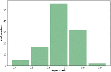 | ||
| Fig. 1 The distribution of aspect ratio values across the materials included in the training data set. Values presented here are the mean values from three measurements. | ||
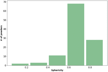
Fig. 2 shows that most of the materials had sphericity greater than 0.5 with 68 of the materials having a sphericity value between 0.6 and 0.8.38
Surface area and energy measurements – Surface Energy Analyser
A representative sample of 35 powders were selected for surface area and surface energy measurement in the training dataset. Surface energy parameters measured were specific surface energy (mJ m−2), surface energy (mJ m−2), and dispersive surface energy (mJ m−2) at 0%, 3%, 5%, and 10% of coverage (see ESI†) (Table 5).| Parameter | Range of values | Mean |
|---|---|---|
| Surface area | 0.17 to 2.76 m2 g−1 | 0.64 m2 g−1 |
| Specific surface energy | 2.94 to 16.81 mJ m−2 | 7.07 ± 0.48 mJ m−2 |
| Surface energy (com) | 0.06 to 140.73 mJ m−2 | 41.62 ± 0.66 mJ m−2 |
Powder flow and bulk density
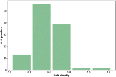
The bulk density and powder flow of the 112 pharmaceutical powders were analysed using Powder Rheometer FT4 – Freeman Technology Ltd. (see Fig. 3 and Table 6). Both types of measurements were done in triplicate.| Flow function coefficient | Powder behaviour | Number of observations |
|---|---|---|
| FFc < 4 | Cohesive | 29 |
| 4 < FFc < 10 | Easy-flowing | 32 |
| FFc > 10 | Free-flowing | 51 |
Using unsupervised and supervised learning methods to predict powder flow
Two types of models, namely a single-step and two-step classification, were investigated using supervised algorithms described in the Machine learning methods section. The first model developed a single-step classification in which materials were classified into one of the three FFc classes described above. The performance of this classification was assessed by calculating AUC–ROC (see Fig. 5). The highest performance achieved was by the multilayer perceptron neural network model (0.823). For classes 1 and 3, over 60% of the instances were correctly classified; however, for class 2, less than 45% of the materials were correctly classified by the model. The model therefore appeared to be better at predicting the FFc classes of cohesive and free-flowing materials but struggled to classify the easy-flowing26 materials across the transition from cohesive to free flowing.
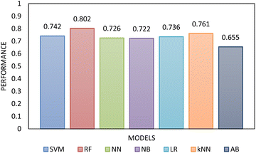 | ||
| Fig. 5 The AUC–ROC performance analysis of the single-step model compared to each other evaluated using 10-fold cross-validation. The highest performance was achieved by RF. | ||
As the MLP neural network confusion matrix indicated that easy-flowing materials were difficult to distinguish from free-flowing materials (see Section 4 of ESI†). A two-step classification model was developed as following Jenike's classification of powder flow:24 Step 1 classified materials into free-flowing (FFc > 10) or non-free-flowing (FFc < 10), cohesive and easy-flowing powders were included in the latter category. Step 2 classified the material into cohesive materials (FFc < 4) and non-cohesive materials (FF > 4), easy-flowing and cohesive powders were included in the latter category. According to the literature, easy and free-flowing powders are suitable for manufacturing with free-flowing powders being most suitable for direct compression.18 The performance of the algorithms included in step 1 and step 2 was again assessed using AUC–ROC (see Fig. 6 and 8). The results showed that by separating the classification decisions, the two-step model was able to perform better than the previous model. This improvement in the performance of the two-step model could be explained by considering that the imbalanced training dataset used for the single-step model affected the performance of the model, and when the dataset was split into subconsequent steps, the detrimental impact of the imbalanced data was minimised.
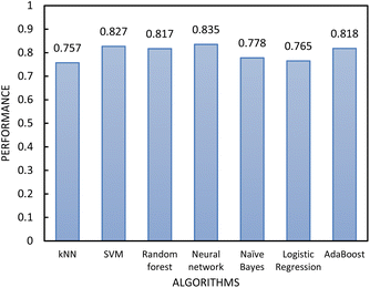 | ||
| Fig. 6 The performance of the classification algorithms included in step 1 of the two-step model evaluated by 10-fold cross-validation. | ||
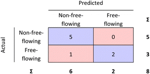 | ||
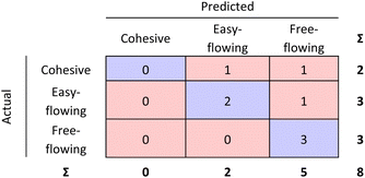
| Fig. 7 External validation performed for the RF model. 87.5% of the materials were correctly classified. | ||
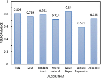 | ||
| Fig. 8 The performance of the classification algorithms included in step 2 of the two-step model evaluated using 10-fold cross-validation. | ||
In determining which algorithm should be used for external validation, we prioritised model performance in step 1 as this classification step (free- vs. non-free-flowing) is more impactful for determining manufacturability than the classification in step 2 (cohesive vs. non-cohesive). For step 1, the neural network model had the highest performance (0.835), followed by RF (0.817). The neural network model was initially used for external validation (see ESI†). However, since the external validation classification accuracy was signficantly worse (62.5%) than the classification accuracy for the test set, we hypothesize that the neural network algorithm was overfitting the data. As the model with the next highest performance, the RF model for both step 1 and 2 was used for all remaining external validation.
The RF confusion matrices for step 1 and step 2 have been combined to have a better overview of the performance of the two-step model (see Fig. 9).
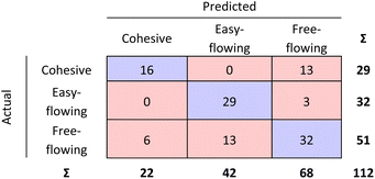 | ||
| Fig. 9 Step 1 and step 2 RF model confusion matrices combined as evaluated by 10-fold cross validation. | ||
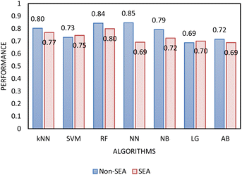
Surface area and surface energy data were also added to the training set of the single-step and the two-step models because it has been previously shown that surface parameters have a significant influence on powder behaviour.39,40 The addition of these parameters resulted in a decrease in model performance for all algorithms, except kNN in step 1, and SVM and LR in step 2. A previous publication also showed that when improved particle size and shape data are available, the addition of surface area and surface energy data does not translate into an improvement of the performance of the model for the prediction of powder flow.23 The decrease in performance due to the addition of more data can be a result of the small correlation between surface area and surface energy with powder flow, because the information introduced to the model is effectively noise. This result suggests that powder flowability is more strongly dependent on size and shape than it on surface area and surface energy. As the addition of these parameters did not improve performance, they were not included in later training datasets (Fig. 10).
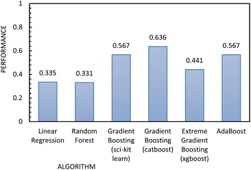 | ||
| Fig. 11 Regression metrics to evaluate the performance of the algorithms used to build the regression model, using FFc as the independent variable. | ||
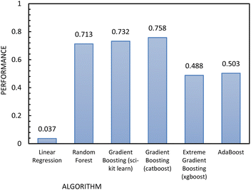
Fig. 12 shows the results of the regression models that have 1/FFc as the dependent variable with performances evaluated by 10-fold cross-validation. From these results, we see that using 1/FFc decreased prediction error compared to the models that predict FFc directly (see Fig. 11). For these models, CatBoost exhibited the best performance, with an R2 value of 0.758, and an RMSE of 0.069.
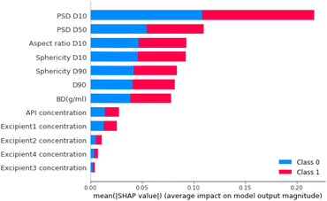
The feature that had the biggest impact on model performance in step 1 PSD D10 (i.e., 10% of the particles have a particle size smaller than this value; Fig. 14). Therefore, this analysis indicated that the model's prediction between free-flowing and non-free-flowing powders was impacted significantly by the presence of fines in the material as captured in the elevated impact of the D10 value.
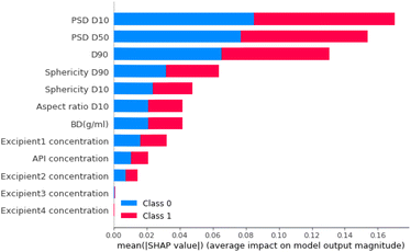
For step 2, the feature importance analysis is also calculated for the neural network model. Fig. 15 shows that, as for the step 1 classifier, PSD D10 is also the most important material feature. Other features that had high importance scores were PSD D50 and PSD D90 (particle size distribution 50% and 90% percentile, respectively). These were also important parameters for Step 1.
SHAP values were calculated using SHAP python library for one of the powder samples that were misclassified in the external validation to examine why the prediction was incorrect. The specific powder was a cohesive material that the external validation classified as free-flowing. This powder's prediction was chosen for SHAP local analysis since the misclassification of a non-free flowing powder as free flowing would result in a waste of both time and material in investigating the manufacturability of this powder. Step 1 classified this powder with a 67% probability (see Fig. 16) as free-flowing, but its measured FFc was 1.9.
Fig. 16 also shows that the feature that had the biggest impact on the model output was again the PSD D10 value of the sample (225.11 μm). This value of PSD D10 is significantly higher than the mean value of PSD D10 of the training set (shown in Table 4). Furthermore, the material displayed high sphericity with a high value of aspect ratio D90 (0.98). Therefore, since the powder had large and spherical particles, these properties may have resulted in this misclassification. Adding additional training data with a wider range of different combinations of particle size and shape with varying bulk properties would help avoid such misclassifications in future models.
From the SHAP value analysis, the model here may slightly inflate the importance of D10 when compared with sphericity values, as the size and aspect ratio were the most important factors in both the correct and incorrect classifications of the materials. Thus, retraining models with more materials with a training set with a greater variance in sphericity could improve the performance.
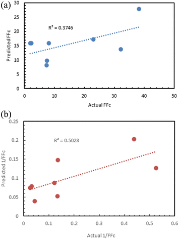
| Actual FFc | Predicted FFc | Actual 1/FFc | Predicted 1/FFc |
|---|---|---|---|
| 1.90 | 15.94 | 0.526 | 0.127 |
| 2.28 | 15.85 | 0.438 | 0.203 |
| 7.42 | 8.24 | 0.135 | 0.148 |
| 7.46 | 9.73 | 0.134 | 0.053 |
| 8.17 | 15.83 | 0.122 | 0.088 |
| 32.14 | 13.78 | 0.031 | 0.079 |
| 38.21 | 27.84 | 0.026 | 0.075 |
| 23.00 | 17.27 | 0.043 | 0.040 |
The prediction against 1/FFc as dependent variable (R2 = 0.5) was better than the prediction of FFc (R2 = 0.37), although neither result was satisfactory (Fig. 17).
Conclusions
Implementing ML models in the early stages of drug development can help determine suitable manufacturing strategies for a given material and provide rapid digital screening tools for advanced pharmaceutical development. In this work, FFc classes of pharmaceutical materials were predicted from routine, widely available, material-sparing analytical measurements. The 112 materials analysed exhibited a wide range of particle size distributions, particle shape distributions, and bulk densities and covered 3 classes of FFc that reflect what is captured in the literature.24This work suggests that particle size and shape distribution measured with dynamic image analysis are sufficient to enable the prediction of flow properties. The best performing model presented in this work was achieved by the combination of RF models for step 1 and step 2, with over 80% probability of distinguishing between classes for each step. Further improvements to model performance could be made with more data from cohesive materials as this would help address class imbalance in the training dataset. Additionally, including training data with different combinations of particle size and shape with differing bulk behaviour could also reduce misclassifications in future models. The FFc boundaries of the classes of powder flow could also be adapted to specific industry needs; for example, optimal FFc values will vary depending on the different pieces of equipment that might be available. In this work, propagation of analytical measurement error has not been included in the model training, and this research angle could be interesting to explore in further work. Moreover, the model could be extended to inform formulation optimization or even to provide a performance target for particle engineering efforts to develop materials for direct compression.
The ML model's implementation enables the prediction of the material flow properties (FFc) from size and shape allowing early decision-making regarding manufacturing route selection. Although there are more sophisticated techniques to capture particle size and shape data, the consideration of the whole particle size and particle shape distribution may allow a better understanding of the data and of the relationship between particle size and shape and powder flow, resulting in a better predictive model. Moreover, the model could be extended to inform formulation optimization or even to provide a performance target for particle engineering efforts to develop materials for direct compression. Implementation of the models presented here in industry applications could save time and effort in early-stage development. The work presented in this paper illustrates the benefits of implementing digital design workflows for the prediction of material properties in the pharmaceutical industry where the availability of data is often limited. This work highlighted multiple potential applications that could result from increasing the available FAIR data in this industry and how it can help to digitalise pharmaceutical manufacturing.
Data availability
All data underpinning this publication are openly available from the University of Strathclyde KnowledgeBase at https://doi.org/10.15129/3005493b-a125-4a5d-8599-525ce952facf. The code supporting this article has been uploaded as part of the ESI.†Author contributions
Laura Pereira Diaz: writing – original draft, data generation, data curation, investigation, methodology, validation. Cameron Brown: review and editing, supervision. Ebenezer Ojo: samples of pharmaceutical mixtures. Chantal Mustoe: review and editing. Alastair Florence: review and editing, supervision.Conflicts of interest
The authors declare that they have no known competing financial interests or personal relationships that could have appeared to influence the work reported in this paper.Acknowledgements
The authors thank EPSRC and the EPSRC Future Continuous Manufacturing and Advanced Crystallisation Research Hub (Grant ref: EP/P006965/1) for funding this work. The authors acknowledge that parts of this work were carried out in the CMAC National Facility supported by a UK Research Partnership Fund (UKRPIF) award from the Higher Education Funding Council for England (HEFCE) (Grant ref HH13054). The authors acknowledge the Medicines Manufacturing Innovation Centre (MMIC) for sharing data. MMIC is co-funded by UK Research and Innovation (UKRI) and the Scottish government and is a collaboration between the public and private sector, including GlaxoSmithKline and AstraZeneca (Innovate UK: 104208 (2018-2021) & 900070 (2017-2018)).References
- J. Maier, UK Industrial Digitalisation Review, 2017 Search PubMed.
- H. Abe, S. Yasui, A. Kuwata and H. Takeuchi, Chem. Pharm. Bull., 2009, 57, 647–652 CrossRef CAS PubMed.
- R. F. Shangraw, Pharm. Dosage Forms: Tablets, 1989, 1, 195–246 Search PubMed.
- B. E. Schaller, K. M. Moroney, B. Castro-Dominguez, P. Cronin, J. Belen-Girona, P. Ruane, D. M. Croker and G. M. Walker, Int. J. Pharm., 2019, 566, 615–630 CrossRef CAS PubMed.
- A. N. Trementozzi, C.-Y. Leung, F. Osei-Yeboah, E. Irdam, Y. Lin, J. M. MacPhee, P. Boulas, S. B. Karki and P. N. Zawaneh, Int. J. Pharm., 2017, 523, 133–141 CrossRef CAS PubMed.
- H. P. Goh, P. W. S. Heng and C. V. Liew, Int. J. Pharm., 2018, 547, 133–141 CrossRef CAS PubMed.
- W. Yu, K. Muteki, L. Zhang and G. Kim, J. Pharm. Sci., 2011, 100, 284–293 CrossRef CAS PubMed.
- U. V. Shah, V. Karde, C. Ghoroi and J. Y. Heng, Int. J. Pharm., 2017, 518, 138–154 CrossRef CAS.
- A. Guo, J. Beddow and A. Vetter, Powder Technol., 1985, 43, 279–284 CrossRef CAS.
- A. Crouter and L. Briens, AAPS PharmSciTech, 2014, 15, 65–74 CrossRef CAS PubMed.
- K. Kunnath, L. Chen, K. Zheng and R. N. Davé, Powder Technol., 2021, 377, 709–722 CrossRef CAS.
- C. Sun and D. J. Grant, Int. J. Pharm., 2001, 215, 221–228 CrossRef CAS PubMed.
- J. S. Kaerger, S. Edge and R. Price, Eur. J. Pharm. Sci., 2004, 22, 173–179 CrossRef CAS PubMed.
- L. J. Bellamy, A. Nordon and D. Littlejohn, Int. J. Pharm., 2008, 361, 87–91 CrossRef CAS PubMed.
- H. Masuda, K. Higashitani and H. Yoshida, Powder Technology Handbook, CRC Press, 2006 Search PubMed.
- A. J. Hlinak, K. Kuriyan, K. R. Morris, G. V. Reklaitis and P. K. Basu, J. Pharm. Innovation, 2006, 1, 12–17 CrossRef.
- B. Y. Shekunov, P. Chattopadhyay, H. H. Tong and A. H. Chow, Pharm. Res., 2007, 24, 203–227 CrossRef CAS PubMed.
- M. Leane, K. Pitt, G. Reynolds and M. C. S. W. Group, Pharm. Dev. Technol., 2015, 20, 12–21 CrossRef CAS PubMed.
- N. Sandler and D. Wilson, J. Pharm. Sci., 2010, 99, 958–968 CrossRef CAS PubMed.
- A. J. Megarry, S. M. E. Swainson, R. J. Roberts and G. K. Reynolds, Int. J. Pharm., 2019, 555, 337–345 CrossRef CAS PubMed.
- M. Capece, K. R. Silva, D. Sunkara, J. Strong and P. Gao, Int. J. Pharm., 2016, 511, 178–189 CrossRef CAS PubMed.
- V. R. Nalluri and M. Kuentz, Eur. J. Pharm. Biopharm., 2010, 74, 388–396 CrossRef CAS.
- H. Barjat, S. Checkley, T. Chitu, N. Dawson, A. Farshchi, A. Ferreira, J. Gamble, M. Leane, A. Mitchell, C. Morris, K. Pitt, R. Storey, F. Tahir and M. Tobyn, J. Pharm. Innovation, 2021, 16, 181–196 CrossRef.
- A. W. Jenike, Bulletin No. 123, Utah State University, 1964 Search PubMed.
- F. T. Ltd, Shear Testing, https://www.freemantech.co.uk/powder-testing/ft4-powder-rheometer-powder-flow-tester/shear-testinghttps://www.freemantech.co.uk/powder-testing/ft4-powder-rheometer-powder-flow-tester/shear-testing, accessed 01/02/2021 Search PubMed.
- J. Zegzulka, D. Gelnar, L. Jezerska, R. Prokes and J. Rozbroj, Sci. Rep., 2020, 10, 1–19 CrossRef.
- W. H. Organization, The International Pharmacopoeia, 2012, vol. 6 Search PubMed.
- J. Lever, Nat. Methods, 2016, 13, 603–605 CrossRef CAS.
- P. Branco, L. Torgo and R. P. Ribeiro, ACM Computing Surveys (CSUR), 2016, vol. 49, pp. 1–50 Search PubMed.
- M. Galar, A. Fernandez, E. Barrenechea, H. Bustince and F. Herrera, IEEE Trans. Syst. Man Cybern. C Appl. Rev., 2011, 42, 463–484 Search PubMed.
- D. C. Montgomery, E. A. Peck and G. G. Vining, Introduction to Linear Regression Analysis, John Wiley & Sons, 2021 Search PubMed.
- F. Sigrist, arXiv, 2018, preprint, arXiv:1808.03064, DOI:10.48550/arXiv.1808.03064.
- Y. Zhang and A. Haghani, Transport. Res. C Emerg. Technol., 2015, 58, 308–324 CrossRef.
- J. K. Jaiswal and R. Samikannu, World Congress on Computing and Communication Technologies (WCCCT), 2017, pp. 65–68 Search PubMed.
- Q. Liu, X. Wang, X. Huang and X. Yin, Tunn. Undergr. Space Technol., 2020, 106, 103595 CrossRef.
- S. M. Lundberg and S.-I. Lee, Adv. Neural Inf. Process. Syst., 2017, 30, 4768–4777 Search PubMed.
- S. Lundberg, Welcome to the SHAP Documentation, accessed 19/05/2022 Search PubMed.
- T. S. Pinto, O. Lima and L. Leal Filho, Min., Metall., Explor., 2009, 26, 105–108 CAS.
- F. Fichtner, D. Mahlin, K. Welch, S. Gaisford and G. Alderborn, Pharm. Res., 2008, 25, 2750–2759 CrossRef CAS PubMed.
- C. G. Jange and R. K. Ambrose, Powder Technol., 2019, 344, 363–372 CrossRef CAS.
Footnote |
| † Electronic supplementary information (ESI) available. See DOI: https://doi.org/10.1039/d2dd00106c |
| This journal is © The Royal Society of Chemistry 2023 |

