Continuum models for directed self-assembly†
Marcus
Müller
 * and
Juan Carlos
Orozco Rey

University of Goettingen, Institute for Theoretical Physics, Friedrich-Hund-Platz 1, 37077 Göttingen, Germany. E-mail: mmueller@theorie.physik.uni-goettingen.de; Fax: +49 551 399631; Tel: +49 551 3913888
First published on 22nd December 2017
Abstract
The computational description of directed self-assembly (DSA) of copolymer materials requires the prediction of large-scale structure formation of copolymer materials guided by chemical or topographical patterns. The disparity between the periodicity of self-assembled structures and the large length scale of devices poses computational challenges that requires the use of highly coarse-grained models. The highest level of coarse-graining is achieved by continuum models that integrate out the molecular degrees of freedom and describe the system only by the local composition. We evaluate the abilities of two continuum models – the Swift–Hohenberg and Ohta–Kawasaki free-energy functionals – to describe directed self-assembly qualitatively and quantitatively by comparison to self-consistent field theory and particle-based simulations, illustrating applications to defect motion and annihilation and the design of guiding patterns for fabricating device-oriented structures. We devise a phenomenological mapping between the Ohta–Kawasaki model and the standard Gaussian chain model of block copolymers, highlight the advantages of the Ohta–Kawasaki model and discuss the significance of the disparity between the characteristic length scale of surface-directed spinodal self-assembly and the equilibrium domain spacing.
Design, System, ApplicationRelevant properties of the directed self-assembly (DSA) of block-copolymers can be predicted using Ohta–Kawasaky model. The computational ease of this continuum model lies on the drastic reduction of degrees of freedom used to represent the block-copolymer system with a collective order parameter instead of using molecular level descriptors. A faster computational screening of the multi-dimensional parameter space can be performed within this model in order to limit the design space to the most promising parameter combination for DSA. More detailed simulation techniques like particle-based simulations or self-consistent field theory (SCFT) can be used to validate the predictions of the continuum model, providing a combined efficient strategy for the multiscale optimization challenge. In spite of the limited description of molecular architecture, the Ohta–Kawasaki model is a valuable tool to provide valuable insights into the processes involved in DSA at the thermodynamical level. |
1 Introduction
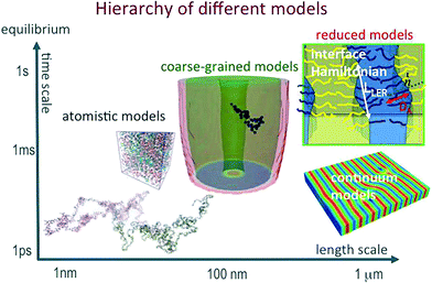
Directed self-assembly (DSA) of copolymer materials has emerged as a promising strategy for templating dense arrays of nanostructures with extremely low defect density and spatial registration with other device components.1–17 In order to fulfill the exacting demands of technological applications much effort has been devoted to (i) optimize the copolymer materials, (ii) tailor the guiding patterns, and (iii) devise processes that mitigate defect formation and facilitate defect annihilation.This is a truly multiscale problem (see Fig. 1):18 AB diblock copolymers are comprised of two, thermodynamically incompatible chain molecules, A and B, that are linked together into a linear macromolecule. The covalent bonding of the two blocks prevents macrophase separation and, instead, the molecules arrange into periodic nanostructures. The symmetry and periodicity is dictated by the balance between the volume fraction f of the A-component, the interface free-energy between the A and B domains and conformational entropy loss due to stretching as the chain molecules uniformly fill space.19–22 The interface tension depends on the details of molecular structure and interactions. The thermodynamic repulsion of the blocks is quantified by the product, χN, of the Flory–Huggins parameter and the number of segments per macromolecule. The conformational entropy loss is set by the ratio (L/Re)2 between the periodicity, L, and the polymer's end-to-end distance, Re. For Gaussian chains,  where b is the statistical segment length. The parameters, χ and b, are determined by the chemical structure of the two components, A and B, and their prediction requires an atomistic description. In the following we assume that both blocks are characterized by the same statistical segment length, b = bA = bB. Moreover, unless stated explicitly, we consider symmetric systems with f = 1/2 that form lamellae in the bulk.
The mean-field description of microphase separation within the standard Gaussian chain model23 does not involve the individual parameters, b, N, and χ but only the coarse-grained invariants, Re and χN that quantifies the thermodynamic incompatibility between the blocks, i.e., the description is invariant under changing the segmentation N of the molecular contour.24–26 Fluctuation effects that give rise e.g., to line-edge roughness (LER) or line-width-roughness (LWR) in lamellar-forming copolymers,27–31 are controlled by the invariant degree of polymerization, ![[scr N, script letter N]](https://www.rsc.org/images/entities/char_e52d.gif) = (ρRe3/N)2, which quantifies the number of polymers a given chain molecule interacts with. ρ denotes the number density of segments. Topographical guiding patterns as well as the free surface of the copolymer film are often represented by hard, impenetrable walls because the width of the surface to the vapor or a solid boundary is much narrower than all other length scales of interest. The preference of surfaces towards one of the copolymer components is often parameterized by the dimensionless difference of surface tension,
= (ρRe3/N)2, which quantifies the number of polymers a given chain molecule interacts with. ρ denotes the number density of segments. Topographical guiding patterns as well as the free surface of the copolymer film are often represented by hard, impenetrable walls because the width of the surface to the vapor or a solid boundary is much narrower than all other length scales of interest. The preference of surfaces towards one of the copolymer components is often parameterized by the dimensionless difference of surface tension,  . Within the standard Gaussian chain model, copolymer materials that are described by the same coarse-grained invariants, f, Re, χN,
 ![[scr N, script letter N]](https://www.rsc.org/images/entities/char_e52d.gif) , and
, and  exhibit the same behavior.26
This universality of copolymer behavior allows one to use highly coarse-grained models where each effective interaction center – bead – corresponds to a large number of chemical repeating units. The relevant interactions – chain connectivity, thermodynamic repulsion between unlike blocks, uniform density, and surface preference – are represented by computationally efficient potentials, e.g., a bead-spring model with harmonic bonds, soft, repulsive interactions between bead, and surface potentials whose range is a small fraction of Re. We choose the strength of these interactions as to reproduce the experimental values of the coarse-grained invariants, Re, χN, ![[scr N, script letter N]](https://www.rsc.org/images/entities/char_e52d.gif) , and
, and  . These top-down coarse-grained models can be studied by self-consistent field theory or particle-based simulation.24–26,32
In order to increase the computational speed even further one can drop the notion of individual molecules altogether and describe the system configuration by collective variables. Two qualitatively different type of approaches have been employed: (i) interface Hamiltonians where the morphology is characterized by the spatial location of the internal AB interfaces20,21,27,33,34 and (ii) continuum free-energy functionals where the morphology is described by the local concentration of A segments.35–50 The former approach is very useful in the strong-segregation regime, χN ≫ 10, and has been successfully applied to study LER.27 Recent applications of DSA, however, focus on small periodicities, L < 20 nm, which requires small N and a careful choice of the chemical structure – high-χ materials – to bring the invariant χN over the mean-field threshold, χNODT ≈ 10.5, where microphase separation can be observed, i.e., systems with small L are typically not in the strong-segregation regime.
Continuum free-energy functionals provide the free energy of the system as a functional of the spatially inhomogeneous, normalized densities, ϕA(r) and ϕB(r). In the technologically important weak-segregation limit, χN ≈ χNODT ≈ 10.5, the free-energy functional can be derived from the standard Gaussian chain model.19,36,37,49 Thus, in this manuscript, we focus on continuum free-energy functionals and critically assess their ability to capture the equilibrium and dynamic properties pertinent to DSA by comparing them to self-consistent field theory (SCFT) and computer simulations of soft, coarse-grained particle models.51–53
2 Continuum models
Continuum models35–50 strike a compromise between retaining some aspects of the predictive power of more detailed molecular models and enabling a computationally screening of the multi-dimensional parameter space and the reverse design of the DSA process specified by (i) the copolymer materials, (ii) the geometry and interactions of the guiding pattern, and (iii) the process conditions that control the kinetics of DSA.Instead of using the molecular degrees of freedom, i.e., positions and momenta of polymer segments, as fundamental descriptors of a microscopic configuration, continuum models operate on a coarser scale and employ a collective order parameter, m. Since a dense AB copolymer melt is nearly incompressible ϕA(r) + ϕB(r) = 1, one often describes the two-component system by a single, spatially varying order parameter, m(r) ∼ ϕA(r) − ϕB(r), that quantifies the difference in the local density of the two components, A and B. Typically the order-parameter field, m(r), is evaluated on a collocation grid, whose spatial discretization is set by the smallest relevant length scale, i.e., the width of the internal AB interfaces. Thus the values of the order parameter at the grid vertices characterize a configuration, giving rise to a drastic reduction in the number of degrees of freedom in comparison to a molecular description. This choice of the order-parameter is common to both continuum models discussed in the following, and it imposes several limitations from the outset:
• Since the use of a single collective order parameter ignores which molecule and which part of it contributes to the density at position r, the quantitative description of architectural effects (e.g., polydispersity, chain-end effects, or homopolymer–copolymer mixtures) is limited.
• The assumption of incompressibility obviously breaks down at the narrow surface of the polymer film to the supporting substrate or the free surface to air/vacuum. More generally, the appropriate formulation of boundary conditions is challenging because the changes of the molecular conformations at a sharp inhomogeneity are not explicitly described.
• Like in dynamic SCFT, one assumes that the chain configurations are always in equilibrium with the instantaneous order parameter and often uses approximations to relate the dynamics of the interacting molecules to the order-parameter kinetics.
Having defined the order parameter, continuum models seek to describe the equilibrium thermodynamics by a free-energy functional, ![[scr F, script letter F]](https://www.rsc.org/images/entities/char_e141.gif) [m]. Two different continuum models are discussed in literature – (i) the Swift–Hohenberg model or phase-field crystal model35–42 and (ii) the Ohta–Kawasaki free-energy functional43–50 – to model the structure and thermodynamics of spatially modulated phases.
[m]. Two different continuum models are discussed in literature – (i) the Swift–Hohenberg model or phase-field crystal model35–42 and (ii) the Ohta–Kawasaki free-energy functional43–50 – to model the structure and thermodynamics of spatially modulated phases.
In principle, ![[scr F, script letter F]](https://www.rsc.org/images/entities/char_e141.gif) [m] can be constructed by comparison to SCFT in the weak-segregation limit (RPA-mapping)19,36,37,49 or simulations of particle-based models in conjunction with field-theoretic umbrella sampling.26,54 In practice, however, phenomenological expressions are employed that represent expansions in terms of powers of the order parameter and its spatial derivatives supplemented by general symmetry considerations and that match the fluctuation spectrum of a copolymer melt in the disordered state. These symmetry considerations specify the free-energy functional in the bulk, and
[m] can be constructed by comparison to SCFT in the weak-segregation limit (RPA-mapping)19,36,37,49 or simulations of particle-based models in conjunction with field-theoretic umbrella sampling.26,54 In practice, however, phenomenological expressions are employed that represent expansions in terms of powers of the order parameter and its spatial derivatives supplemented by general symmetry considerations and that match the fluctuation spectrum of a copolymer melt in the disordered state. These symmetry considerations specify the free-energy functional in the bulk, and ![[scr F, script letter F]](https://www.rsc.org/images/entities/char_e141.gif) [m] is augmented by terms that describe the interaction with the guiding pattern and boundary conditions. The minima of
[m] is augmented by terms that describe the interaction with the guiding pattern and boundary conditions. The minima of ![[scr F, script letter F]](https://www.rsc.org/images/entities/char_e141.gif) [m] specify the equilibrium morphologies and allow for the construction of the equilibrium phase diagram of confined copolymer systems.
[m] specify the equilibrium morphologies and allow for the construction of the equilibrium phase diagram of confined copolymer systems.
The relation between the dynamics of the individual macromolecules in the course of the ordering process and the collective kinetics of structure formation, i.e., the time-evolution of m(r,t) is routinely parameterized by an Onsager coefficient,. This Onsager coefficient quantifies the order-parameter current, j(r) that is generated by a gradient of the chemical potential, μ(r) = δ![[scr F, script letter F]](https://www.rsc.org/images/entities/char_e141.gif) /δm(r). Formal expressions for Λ can be derived, e.g., Λ ∼ ϕA(r)ϕB(r) to account for incompressibility or Λ ∼ g(r,r′) where g denotes the intramolecular correlation function, but computing Λ is a formidable task.55–57 Routinely, drastic approximations, e.g., ignorance of composition-dependence and non-locality of Λ, are employed, resulting in:
/δm(r). Formal expressions for Λ can be derived, e.g., Λ ∼ ϕA(r)ϕB(r) to account for incompressibility or Λ ∼ g(r,r′) where g denotes the intramolecular correlation function, but computing Λ is a formidable task.55–57 Routinely, drastic approximations, e.g., ignorance of composition-dependence and non-locality of Λ, are employed, resulting in:
| j(r) = −Λ∇μ(r) | (1) |
This current and the time evolution of the order parameter are connected via the continuity equation, which the conservation of the species A and B also imparts onto m, resulting in a conserved Cahn–Hilliard dynamics for the order parameter (model B according to the classification of dynamic universality classes according to Hohenberg and Halperin58).
 | (2) |
In this simple form, Λ is a constant and can be adsorbed as a scale factor of time. Different numerical schemes have been devised to integrate this partial differential equation in time. In our exploratory study we use the simple forward Euler scheme.
2.1 Self-consistent field theory (SCFT)
In the limit of large![[scr N, script letter N]](https://www.rsc.org/images/entities/char_e52d.gif) , the thermodynamics of block copolymer structures can be accurately described by self-consistent field theory (SCFT).59–63 This approach has been successfully used to study the phase diagram,22,23 defect properties16,17,53 and the minimum free-energy path of defect annihilation.51,64 Within SCFT the statistical mechanics of interacting macromolecules is approximated by the properties of non-interacting chain molecules in self-consistently determined, external fields, wA(r) and wB(r), acting on the A blocks and B blocks, respectively. Given wA(r) and wB(r), the most probable densities of non-interacting Gaussian chain molecules subjected to the external fields,
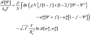
, the thermodynamics of block copolymer structures can be accurately described by self-consistent field theory (SCFT).59–63 This approach has been successfully used to study the phase diagram,22,23 defect properties16,17,53 and the minimum free-energy path of defect annihilation.51,64 Within SCFT the statistical mechanics of interacting macromolecules is approximated by the properties of non-interacting chain molecules in self-consistently determined, external fields, wA(r) and wB(r), acting on the A blocks and B blocks, respectively. Given wA(r) and wB(r), the most probable densities of non-interacting Gaussian chain molecules subjected to the external fields, | (3) |
 , can be computed via a modified diffusion equation.59–63 Here
  denotes the single-chain partition function of a diblock copolymer in volume V subjected to the external fields, wA and wB. Inverting this relation, one obtains the external fields,
  and
and  , that correspond to a given order parameter, Ψ(r) = ϕA(r) – f and satisfy the incompressibility constraint, ϕA(r) + ϕB(r) = 1. SCFT yields the following estimate for the free-energy functional
 | (4) |
 and
and  .
.
Here we use the spectral approach62 to compute the equilibrium properties of lamellae formed by symmetric diblock copolymers, f = 0.5, that serve as accurate reference data to gauge the accuracy of the continuum models. Minimizing the free-energy functional, eqn (4), yields the self-consistency condition for the order parameter
 | (5) |
![[scr F, script letter F]](https://www.rsc.org/images/entities/char_e141.gif) [Ψ*] and, minimizing the equilibrium free energy, F, with respect to the periodicity, we estimate the equilibrium domain spacing, L0.
[Ψ*] and, minimizing the equilibrium free energy, F, with respect to the periodicity, we estimate the equilibrium domain spacing, L0.
2.2 Random-phase-approximation (RPA)
In principle, an accurate free-energy functional,![[scr F, script letter F]](https://www.rsc.org/images/entities/char_e141.gif) , can be numerically obtained by SCFT. If the local A density ϕA(r) only deviates slightly from its average f, one can systematically expand the free-energy in terms of the order parameter, Ψ(r) = ϕA(r) − f. This Random-phase-approximation (RPA) yields for the free-energy difference with respect to the homogeneous state, Ψ(r) = 0,19,36,37,49
, can be numerically obtained by SCFT. If the local A density ϕA(r) only deviates slightly from its average f, one can systematically expand the free-energy in terms of the order parameter, Ψ(r) = ϕA(r) − f. This Random-phase-approximation (RPA) yields for the free-energy difference with respect to the homogeneous state, Ψ(r) = 0,19,36,37,49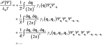 | (6) |
 is the Fourier transform of the order parameter. Both continuum models are based on this fourth-order expansion, eqn (6). The RPA of Leibler19 provides explicit expressions for the wavevector-dependent vertex functions, γi. Both continuum models neglect the wavevector dependence of the vertex functions γ3 and γ4. For the symmetric case, one obtains
  and
and  . Within mean-field approximation, this second-order vertex function is directly related to the collective structure factor in the disordered phase,
  , and takes the explicit form
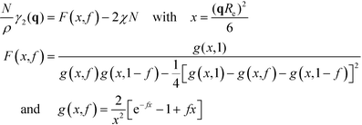 | (7) |
The function F(x,f) describes the influence of the chain conformations on the collective composition fluctuations, and g(x,f) is the Debye function that describes the Gaussian conformational statistics of an individual block. For a symmetric block copolymer, the vertex function exhibits a minimum at x* ≈ 3.7852 or L = 2π/q* ≈ 1.32Re and adopts the value
 | (8) |
The two continuum models differ in the approximation used for the second-order vertex function. The Swift–Hohenberg model approximates γ2(q) by a parabola around q*
 | (9) |
The Ohta–Kawasaki model43 additionally captures the asymptotic behavior for small and large wavevectors
 | (10) |
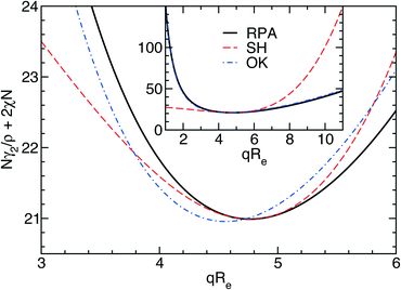
The three forms of the wavevector-dependent second-order vertex functions are depicted in Fig. 2. The Swift–Hohenberg model provides an excellent approximation in the ultimate vicinity of the minimum but yields only a poor representation of the vertex function for large and small wavevectors. The Ohta–Kawasaki model, in turn, accurate captures the asymptotic behavior of the vertex function for q → 0 and q → ∞, as well as the value of the vertex function at its minimum, but it slightly underestimates the position of the minimum,  .
.
2.3 Swift–Hohenberg model
Using the parabolic approximation of the vertex function, one obtains the Swift–Hohenberg model for symmetric block copolymers:35–42 | (11) |
In the following, we introduce units of length ξ0, energy η0, and order parameter Ψ0, and define the dimensionless, rescaled variables
 | (12) |
Relating the units of the continuum models to the coarse-grained invariants via
 | (13) |
 | (14) |
 | (15) |
 | (16) |
 | (17) |
 | (18) |
The Swift–Hohenberg free-energy functional captures the minimal ingredients that are relevant for describing spatially modulated phases. It has been employed to study the universal aspects of structure formation in systems with different underlying interactions (Rayleigh–Bénard convection, magnetic garnets, Turing patterns, lipid membranes, diblock copolymers).40 The model has also attracted recent interest under the name of phase field crystal (PFC) model,39 and it has also been studied in the case that the spatial average of the order parameter, ![[m with combining overline]](https://www.rsc.org/images/entities/i_char_006d_0305.gif) , does not vanish.
, does not vanish.
From eqn (17) we calculate the chemical potential and the equation of motion
 | (19) |
 | (20) |
The Swift–Hohenberg model can reproduce the qualitative phase behavior of block copolymers in the weak segregation limit and it is the computationally simplest form to describe spatially modulated phases. The local character of the free-energy functional enables a rather straightforward computation of the free energy. These attractive properties have made the model rather popular for studying the universal, qualitative features of spatially modulated phases and the kinetics of structure formation.
The parameter ![[small epsilon, Greek, tilde]](https://www.rsc.org/images/entities/i_char_e0de.gif) dictates the equilibrium properties. The disordered structure, m(r) =
dictates the equilibrium properties. The disordered structure, m(r) = ![[m with combining overline]](https://www.rsc.org/images/entities/i_char_006d_0305.gif) , becomes unstable for
, becomes unstable for ![[small epsilon, Greek, tilde]](https://www.rsc.org/images/entities/i_char_e0de.gif) > 3
> 3![[m with combining overline]](https://www.rsc.org/images/entities/i_char_006d_0305.gif) 2, i.e., for a symmetric diblock copolymer with
2, i.e., for a symmetric diblock copolymer with ![[m with combining overline]](https://www.rsc.org/images/entities/i_char_006d_0305.gif) = 0, for
= 0, for ![[small epsilon, Greek, tilde]](https://www.rsc.org/images/entities/i_char_e0de.gif) > 0. For a symmetric bulk system,
> 0. For a symmetric bulk system, ![[m with combining overline]](https://www.rsc.org/images/entities/i_char_006d_0305.gif) = 0, in the weak-segregation limit 0 <
= 0, in the weak-segregation limit 0 < ![[small epsilon, Greek, tilde]](https://www.rsc.org/images/entities/i_char_e0de.gif) ≪ 1, the order-parameter profile can be described by a single Fourier component (one-mode approximation),
≪ 1, the order-parameter profile can be described by a single Fourier component (one-mode approximation),
 | (21) |
![[small epsilon, Greek, tilde]](https://www.rsc.org/images/entities/i_char_e0de.gif) 2V/(6ξ3).
2V/(6ξ3).
The phase diagram of the Swift–Hohenberg model exhibits a tricritical point42 at ![[small epsilon, Greek, tilde]](https://www.rsc.org/images/entities/i_char_e0de.gif) tri = 9/38 and
tri = 9/38 and  . Beyond this tricritical point, it predicts a macrophase coexistence between a spatially modulated phase and a homogeneous phase separated by a miscibility gap. Obviously such phase coexistence cannot occur in a pure block copolymer melt. Thus the model can qualitatively describe pure diblock copolymers only for small
 ![[small epsilon, Greek, tilde]](https://www.rsc.org/images/entities/i_char_e0de.gif) and compositional asymmetries |
and compositional asymmetries |![[m with combining overline]](https://www.rsc.org/images/entities/i_char_006d_0305.gif) |.
|.
From the computational perspective, the Swift–Hohenberg model is the simplest free-energy model. The main difficulty is the high-order spatial derivative in the kinetic equation that enforces a rather small time step, Δt ∼ Δx6, for simple integration schemes to remain numerically stable. In our numerical performance test, we studied the kinetics of structure formation from a disordered to a lamellar structure at very weak segregation, ε = 0.02, and rather coarse spatial discretization, Δx = 0.3140, with a time step of Δt = 0.0003.
2.4 Ohta–Kawasaki model
Using the asymptotically exact approximation, eqn (10), of the second-order vertex function, one derives the Ohta–Kawasaki model for a symmetric block copolymer | (22) |
The long-range kernel, G(r,r), obeys the Poisson equation
−ΔG(r,![[thin space (1/6-em)]](https://www.rsc.org/images/entities/char_2009.gif) r′) = δ(r − r′) + const r′) = δ(r − r′) + const | (23) |
G decays with distance r like 1/r in three spatial dimensions, G ∼ ln(r) in two dimensions, and  for a one-dimensional variation of the order parameter, m(x), with period L.
Relating the units of length, order parameter, and energy, defined in eqn (12), to the coarse-grained invariants according to
 | (24) |
 | (25) |
 | (26) |
 | (27) |
 | (28) |
 | (29) |
![[small gamma, Greek, tilde]](https://www.rsc.org/images/entities/char_e0dd.gif) = 0 for symmetric copolymers = 0 for symmetric copolymers | (30) |
The calculation of the free energy of a configuration, m(r), can be conveniently performed in Fourier space, where the convolution with the long-range kernel, G, reduces to a multiplication. The model also predicts hexagonal and spherical phases, and it does not suffer from the spurious macrophase separation of the Swift–Hohenberg model.
From eqn (28) we calculate the chemical potential and the equation of motion
 | (31) |
 | (32) |
The use of a local Onsager coefficient and the property, eqn (23), of the non-local kernel, G, gives rise to a computationally convenient form of the time-evolution equation that only involves fourth-order spatial derivatives.
For a symmetric bulk system, ![[small gamma, Greek, tilde]](https://www.rsc.org/images/entities/i_char_e0dd.gif) = 0, in the weak-segregation limit
= 0, in the weak-segregation limit  , the order-parameter profile can be described by a single Fourier component (single-mode approximation), mOK–OMA(x) = m0
![[thin space (1/6-em)]](https://www.rsc.org/images/entities/char_2009.gif) sin(2πx/L0), with amplitude and periodicity
sin(2πx/L0), with amplitude and periodicity
 | (33) |
 .
.
In the opposite limit of strong segregation,  , one can approximate the order-parameter profile by a sequence of wide, alternating domains that are separated by narrow AB interfaces. The profile of an individual AB interface is obtained by optimizing the local and square-gradient contribution to the free-energy functional. This yields the same profile as the corresponding homopolymer interface, i.e.,
  (in rescaled units).43 The interfaces are characterized by a tension of
  . To evaluate the long-range contribution, one approximates the interface profile by a sharp-kink profile
 | (34) |
Optimizing the total free energy with respect to the lamellar periodicity, L0, one obtains43,49,50
 | (35) |
3 Results and discussion
In the following we consider symmetric diblock copolymers, f = 1/2 (i.e.,![[small gamma, Greek, tilde]](https://www.rsc.org/images/entities/i_char_e0dd.gif) = 0), and compare the description of the two continuum models with the prediction of SCFT.
= 0), and compare the description of the two continuum models with the prediction of SCFT.
3.1 Free energy and domain spacing
In the vicinity of the order–disorder transition (ODT) the RPA-mapping between the coarse-grained invariants and the parameters of the continuum models is supposed to be accurate. A first, crude estimate of the range of validity of the RPA-mapping can be obtained by requiring that |Ψ| < f = 1/2. Using eqn (14) and (21) for the Swift–Hohenberg model, we find that . Using eqn (18) we obtain the condition χN < 12.9. By the same token, eqn (25) and (33) also yield the condition
  for the Ohta–Kawasaki model.
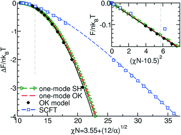
In Fig. 3 we quantitatively compare the free-energy difference per copolymer molecule between the lamellar and disordered phases obtained by the two continuum models and SCFT.
 | (36) |
In the inset of the figure we demonstrate that in the ultimate vicinity of the ODT, indeed, the predictions of the two continuum models in conjunction with the RPA mapping quantitatively agree. The free-energy difference quadratically depends on the distance, χN −10.5 from the ODT because the transition is of second-order within the mean-field treatment. As expected from the rational above, the agreement significantly deteriorates for incompatibilities larger than χN = 12.9; this limit is indicated by the vertical dashed line.
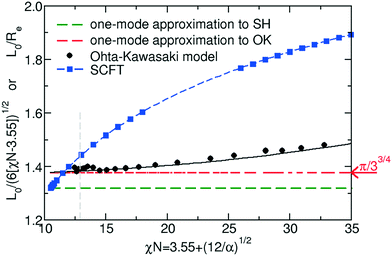
In Fig. 4 we compare the preferred lamellar spacing in units of the unperturbed end-to-end distance, Re.
 | (37) |
Within the one-mode approximation of the Swift–Hohenberg model, the lamellar spacing does not vary with incompatibility and, by construction, agrees with the SCFT value at the ODT. The Ohta–Kawasaki model, in turn, slightly overestimates the lamellar spacing at the onset of ordering because the location of the minimum of γ2 is underestimated (cf.Fig. 2). Within the one-mode approximation we obtain from eqn (35) and (24) also a χN-independent lamellar period,  . Beyond the one-mode approximation, the lamellar spacing increases but the comparison with the SCFT calculation reveals that the dependence of L0 on incompatibility is significantly different already at intermediate values of χN.
From this comparison in Fig. 3 and 4, we conclude that both continuum models in conjunction with the RPA-mapping provide a quantitative description of lamella-forming diblock copolymers in the ultimate vicinity of the ODT, χN < 12.9, but fail to predict the free energy and domain spacing at intermediate and large segregation strengths.
Although novel high-χ materials, which are intensely explored to fabricate structures with the smallest feature sizes, are characterized by small N (and therefore also small χN), this ultimate vicinity of the ODT is only of limited practical use because the high-χ materials are also characterized by small values of the invariant degree of polymerization, ![[scr N, script letter N]](https://www.rsc.org/images/entities/char_e52d.gif) . Thus fluctuation effects become important. One hallmark of fluctuations is the shift of the ODT36 to larger values of incompatibility,
. Thus fluctuation effects become important. One hallmark of fluctuations is the shift of the ODT36 to larger values of incompatibility,  . Thus, for a polymer system with
 ![[scr N, script letter N]](https://www.rsc.org/images/entities/char_e52d.gif) < 5000 the ODT is shifted to values larger than χN = 12.9, and there is no interval of incompatibilities whatsoever, where any of the two continuum models in conjunction with the RPA-mapping provides an accurate, quantitative description. Using generic values of 1 g cm−3 for the density of the melt, and a statistical segment of mass 100 g mol−1 and length b = 0.7 nm, we extract the number density, ρ, of segments and obtain
< 5000 the ODT is shifted to values larger than χN = 12.9, and there is no interval of incompatibilities whatsoever, where any of the two continuum models in conjunction with the RPA-mapping provides an accurate, quantitative description. Using generic values of 1 g cm−3 for the density of the melt, and a statistical segment of mass 100 g mol−1 and length b = 0.7 nm, we extract the number density, ρ, of segments and obtain  , i.e., a polymer with
 ![[scr N, script letter N]](https://www.rsc.org/images/entities/char_e52d.gif) < 5000 is comprised of less than 1167 segments and is characterized by Re < 23.9 nm or L0 < 31.5 nm.
< 5000 is comprised of less than 1167 segments and is characterized by Re < 23.9 nm or L0 < 31.5 nm.
3.2 Metastability of defects
The previous section demonstrated that the two continuum models in conjunction with the RPA-mapping quantitatively describe the self-assembly of block copolymers only in the ultimate vicinity of the ODT, χN < 12.9. Here we explore whether the two models are able to capture the qualitative behavior at intermediate and larger segregation.First, we note that the Swift–Hohenberg model for asymmetric composition predicts a macroscopic phase separation between a disordered phase and a spatially modulated one that differ in their compositions.42 Such a macroscopic phase separation is obviously impossible in a diblock melt because the chain connectivity prevents macroscopic fluctuations of the order parameter. The 1/q2-term in the Ohta–Kawasaki model, in turn, does not allow for macroscopic fluctuations of the order parameter, i.e., the model can only exhibit spatially modulated phases.
Second, SCFT calculations51 and molecular simulations52,53,65 have demonstrated that tight pairs of dislocations are only stable above a threshold of incompatibility, χN* ≈ 18. For smaller incompatibilities, these prototypical defect pairs spontaneously annihilate – providing an important strategy for defect-free DSA.51 We have investigated the metastability of a tight dislocation pair in the Swift–Hohenberg model and the Ohta–Kawasaki model. In the Swift–Hohenberg model, tight dislocation pairs are metastable for ![[small epsilon, Greek, tilde]](https://www.rsc.org/images/entities/i_char_e0de.gif) ≥ 0.5, which corresponds to χN ≈ 12.2 according to the RPA mapping, eqn (18). For values of
≥ 0.5, which corresponds to χN ≈ 12.2 according to the RPA mapping, eqn (18). For values of ![[small epsilon, Greek, tilde]](https://www.rsc.org/images/entities/i_char_e0de.gif) ≤ 0.4, the defect is unstable. In the Ohta–Kawasaki model, in turn, the tight dislocation pair becomes unstable for
≤ 0.4, the defect is unstable. In the Ohta–Kawasaki model, in turn, the tight dislocation pair becomes unstable for ![[small alpha, Greek, tilde]](https://www.rsc.org/images/entities/i_char_e0dc.gif) ≥ 0.80. Using the RPA-mapping, the model parameter corresponds to χN = 15.8, in rather good agreement with SCFT.
≥ 0.80. Using the RPA-mapping, the model parameter corresponds to χN = 15.8, in rather good agreement with SCFT.
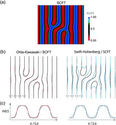
Third, we investigate the ability of continuum models to capture the geometry of the defect morphology. Fig. 5 presents the local density of A-segments, ϕA(x), of a metastable, tight dislocation pair in the lamellar phase of a symmetric diblock copolymer, obtained by SCFT calculations (a) and the corresponding equivalent morphology obtained as a local minimum of the free-energy functional of the Ohta–Kawasaki and Swift–Hohenberg models. From the order-parameter profiles of the morphology in the continuum models, the location of the AB interfaces can be extracted, and we focus on these interface positions in order to compare the description of the geometry within the models.
In the region between the two edge dislocations, the Swift-Hohenberg model predicts a wider lamella between the defect cores and a larger distance D between them (cf. blue contour lines in panel b of Fig. 5). The low accuracy in the description of the morphology by the Swift-Hohenberg model is corroborated by the comparison of the interface profiles far away from the defects, where the model predicts a significantly wider interface with respect to SCFT calculations. Due to the prediction of a spurious macrophase separation and the qualitative failure to capture the morphology of prototypical defects, we focus the following discussion on the Ohta–Kawasaki model.
The results of the Ohta–Kawasaki model, in contrast, agree significantly better with the geometry of the defect predicted by SCFT. Additionally, the composition profiles across a lamella are much better reproduced, when measuring the length scales in units of the preferred lamellar spacing and adjusting the range of the order parameter.
Previously, we have hypothesized that the metastability of defects at intermediate segregation is related to the separation of the intrinsic width, w, of the internal AB interfaces between the domains and the periodicity, L0.51 SCFT at strong segregation, χN ≫ 10, predicts  and
and  , i.e., the ratio of the two lengths scales like
  . In the Ohta–Kawasaki model, we obtain
  , i.e., independent from
 ![[small alpha, Greek, tilde]](https://www.rsc.org/images/entities/i_char_e0dc.gif) , whereas the periodicity increases like
, whereas the periodicity increases like  for
for ![[small alpha, Greek, tilde]](https://www.rsc.org/images/entities/i_char_e0dc.gif) → 0. Thus, the ratio,
→ 0. Thus, the ratio,  , of the two length scales of the lamellar profile decreases for strong segregation,
 ![[small alpha, Greek, tilde]](https://www.rsc.org/images/entities/i_char_e0dc.gif) → 0, and the Ohta–Kawasaki model qualitatively captures the length-scale separation of the SCFT.
→ 0, and the Ohta–Kawasaki model qualitatively captures the length-scale separation of the SCFT.
3.3 Phenomenological extension of mapping for the Ohta–Kawasaki model
The failure of the Ohta–Kawasaki model in conjunction with the RPA-mapping to quantitatively predict the behavior of block copolymers at intermediate and strong segregations is not unexpected because the description is based on the truncation of the systematic expansion, eqn (7), and additional approximations of the wavevector-dependence of the vertex functions. In order to systematically extend the validity of the continuum models, we have to include higher-order terms in the expansion. Whereas several authors have improved the local term in the free-energy functional, to the best of our knowledge, the wavevector-dependence of higher-order vertex functions have not been considered. Such wavevector-dependent vertex functions, however, would result in a rather complex model in real-space representation, and much of the computational benefit of the continuum models (compared to SCFT or single-chain-in-mean-field simulations) would be sacrificed.Therefore, motivated by the universality of self-assembly phenomena and the ability of the Ohta–Kawasaki models to qualitatively capture some of the salient features of block-copolymer self-assembly, we will follow a different strategy: rather than modifying the functional form of the free-energy functional, we merely adjust the mapping of the length scale, ξ0, the order-parameter scale, Ψ0, and the free-energy scale, η0. Thus, we replace the RPA-mapping between the scales, ξ0, Ψ0, η0, and parameters, ![[small alpha, Greek, tilde]](https://www.rsc.org/images/entities/i_char_e0dc.gif) ,
, ![[small gamma, Greek, tilde]](https://www.rsc.org/images/entities/i_char_e0dd.gif) of the continuum model by a phenomenological relation.
of the continuum model by a phenomenological relation.
The amplitude, Ψ0, of the order parameter at intermediate and strong segregation is chosen so that  . Rather than obtaining the scale factors for the free energy and length scales from the RPA-mapping, we use the data in Fig. 3 and 4 in conjunction with eqn (36) and (37). By construction, this procedure eliminates the deviations in Fig. 3 and 4, i.e., the free-energy difference, ΔF, between the lamellar phase and the disordered structure and the lamellar periodicity, L0, agrees with the results of the SCFT of the molecular model.
By virtue of symmetry, we expect that ![[small gamma, Greek, tilde]](https://www.rsc.org/images/entities/i_char_e0dd.gif) = 0 for lamella-forming diblock copolymers with
= 0 for lamella-forming diblock copolymers with  . In the context of DSA, we choose to adjust the value of
 ![[small alpha, Greek, tilde]](https://www.rsc.org/images/entities/i_char_e0dc.gif) so that the phenomenological extension of the mapping captures the excess free energy of a tight dislocation pair. To this end, we have numerically adjusted
so that the phenomenological extension of the mapping captures the excess free energy of a tight dislocation pair. To this end, we have numerically adjusted ![[small alpha, Greek, tilde]](https://www.rsc.org/images/entities/i_char_e0dc.gif) (χN) and the result of this procedure is shown in Fig. 6.
(χN) and the result of this procedure is shown in Fig. 6.
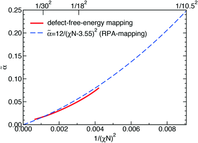 | ||
Fig. 6 Phenomenological extension of the mapping, ![[small alpha, Greek, tilde]](https://www.rsc.org/images/entities/i_char_e0dc.gif) (χN), as to reproduce the excess free energy of a metastable tight dislocation pair. The result is compared with the RPA-mapping, eqn (29). (χN), as to reproduce the excess free energy of a metastable tight dislocation pair. The result is compared with the RPA-mapping, eqn (29). | ||
We observe rather good agreement with eqn (29), suggesting that the ad hoc rescaling of the free-energy and length scales does not give rise to significant artifacts. Thus, we conclude that the Ohta–Kawasaki model in conjunction with the parameter identification provides an appropriate description of DSA of symmetric block copolymers.
To obtain a qualitative understanding of this phenomenological extension, we consider the naive extrapolation of the RPA-mapping to large χN or small ![[small alpha, Greek, tilde]](https://www.rsc.org/images/entities/i_char_e0dc.gif) , respectively. Eqn (29) and (24) suggest the leading-order behavior
, respectively. Eqn (29) and (24) suggest the leading-order behavior ![[small alpha, Greek, tilde]](https://www.rsc.org/images/entities/i_char_e0dc.gif) ≈ 12(χN)−2 and
≈ 12(χN)−2 and  . Using these extrapolations, we find
  and
and  , i.e., the qualitative asymptotic scaling behavior of the width of the intrinsic interface and the domain spacing in the strong segregation limit are reproduced by the Ohta–Kawasaki model (in conjunction with the extrapolated RPA-mapping). Thus, the phenomenological extension changes the prefactors but not the leading χN-dependence of the length scale, ξ0, and the model parameter,
 ![[small alpha, Greek, tilde]](https://www.rsc.org/images/entities/i_char_e0dc.gif) .
.
In the strong-segregation limit, the maximal values of the order parameter, maxx|m(x)|, are ![[scr O, script letter O]](https://www.rsc.org/images/entities/char_e52e.gif) (1), independent of χN. Thus, in contrast to eqn (25), the scale factor Ψ0 will adopt a χN-independent value at large segregation. This scaling behavior will also affect the scale of the free energy. Using eqn (26) in conjunction with Ψ0 ∼ 1 and ξ0/Re ∼ (χN)−1/2, we obtain
(1), independent of χN. Thus, in contrast to eqn (25), the scale factor Ψ0 will adopt a χN-independent value at large segregation. This scaling behavior will also affect the scale of the free energy. Using eqn (26) in conjunction with Ψ0 ∼ 1 and ξ0/Re ∼ (χN)−1/2, we obtain  . Using these modified scale factors and the asymptotic behavior of the Ohta–Kawasaki model in the strong-segregation limit, we obtain for the AB interface tension, σ, and the excess free energy, Δflam, of a copolymer in the lamellar phase,
  and
and  , which agree with the limit of SCFT for large χN, i.e.,
  and
and  , respectively.20,59
3.4 Description of kinetics of structure formation
In the following we illustrate applications of the Ohta–Kawasaki model to defect structures and non-bulk morphologies, for a symmetric diblock copolymer within the technologically relevant, intermediate segregation regime. Model parameters correspond to χN ≈ 30:![[small alpha, Greek, tilde]](https://www.rsc.org/images/entities/i_char_e0dc.gif) = 0.0172 and
= 0.0172 and ![[small gamma, Greek, tilde]](https://www.rsc.org/images/entities/i_char_e0dd.gif) = 0.
= 0.
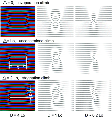
In the following, we study the defect kinetics of apposing dislocations pairs in a lamellar structure using the Ohta–Kawasaki model with Cahn–Hilliard dynamics, eqn (32). We focus on the climb motion of a dislocation pair, which has been studied by experiment66 and simulation.53 Dislocations with apposing Burgers vectors attract each other. Since the glide motion perpendicular to the stripes cannot occur in our model, the distance, Δ, perpendicular to the stripes – the impact parameter – is conserved, whereas the distance, L, along the stripes decreases in response to the strain-field mediated interaction (Peach–Koehler forces) between the dislocation cores.
In our study of defect motion we investigate three different values of the impact parameter, Δ, between defect cores: Δ/L0 = 0,1, and 2, where L0 = 18.28 ξ0 is the equilibrium domain spacing of the bulk lamellae. The dimension in the direction perpendicular to the stripes is set to Ly = NpL0 with Np = 8. Thus, the defect-free lamellar structure is stress-free. The value Np = 8 is larger than or comparable to the distance between chemical guiding patterns in chemoepitaxy with density multiplication or the distance between topographical features in graphoepithaxy, respectively. Periodic boundary conditions are used in our simulations, mimicking the confining effect of chemical or topographical guiding patterns in DSA with Np-fold density multiplication; the pinning of the internal AB interfaces of the lamellae at the guiding pattern is not considered.
For all three cases, the initial dislocation pair is unstable, and the defect cores spontaneously approach each other, i.e., D decreases. Fig. 7 shows the morphology at different stages during the climb motion. For the cases, Δ/L0 = 0 and 1, dislocations collide and annihilate, forming a defect-free lamellar structure. The morphologies before the annihilation, D ≈ 0.2L0, differ: for Δ/L0 = 0 the enclosed extra domain continuously shrinks, whereas for Δ/L0 = 1, the two domain ends are brought into apposition and join, cf. contour lines for D ≈ 0.2L0 in Fig. 7. In the case of Δ/L0 = 2, a metastable tight dislocation pair is formed, and a final finite value of D > 0 remains after the two dislocations pass by each other. We denote this motion as stagnation climb, where the motion stagnates and the system reaches a metastable state, in which the force between the defects vanishes. These observations of the two-dimensional Ohta–Kawasaki model are in agreement with simulations and SCFT calculations.53
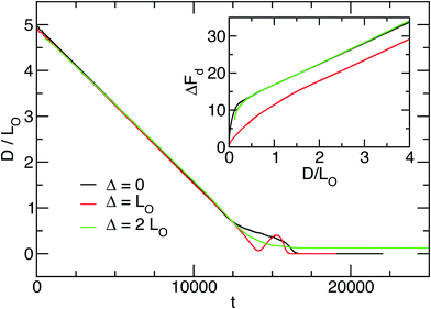
In order to study the velocity of the defect motion in the direction parallel to the lamellae – dislocation climb – we compute the excess free energy, ΔFd, of the defect with respect to the defect-free lamella as a function of D. The results are presented in Fig. 8.
Based on the attractive force between defect cores K = −dΔFd/dD, two regimes of defect motion can be identified: an initial stage where the force is largely independent from the distance, D, between cores, and a final stage where the magnitude of K increases as D approaches zero. The force, K, is distance-independent for values of D > 2L0 in all three cases. For the evaporation and the stagnation climbs, Δ/L0 = 0 and 2, this regime even extends to D > L0. The distance-independence of the attractive force and the limiting value of D > 2L0 for this regime are nicely in agreement with predictions from the minimum free-energy pathway (MFEP) obtained by SCFT calculations53 for the climb motion of dislocation pairs.
In the constant-force regime, the velocity of defect motion is virtually independent from the impact parameter Δ: dD/dt = 1/2930 for the evaporation climb, dD/dt = 1/2900 for the unconstrained climb and dD/dt = 1/3000 in the case of the stagnation climb. This observation differs from particle-based Monte-Carlo simulations,53 where a factor of 25 is observed between the defect annihilation time for Δ = 0 and Δ = L0, the later being faster. We can rationalize this difference by considering our choice of the Onsager coefficient. According to eqn (32), the Onsager coefficient is independent of the order-parameter. This choice does not captures the barrier in the single-chain dynamics, protracting the evaporation of segments from the encircled domain between the defect cores in the case of Δ = 0. Such an intrinsically slow process can be captured by an Onsager coefficient that is proportional to (1 − m)(1 + m), accounting for the incompressibility of the copolymer melt. Unfortunately, this more appropriate choice of the Onsager coefficient makes the dynamic equation – the equivalent to eqn (32) – non-local, posing a computational burden.
 , of two dislocations in the bulk. In previous work,53 we have rationalized this observation by noting that the lamellae between the apposing dislocation cores – the inner region – are compressed due to the presence of an additional stripe, i.e., their lamellar spacing is
  , where L = Ly/Np = L0 is the periodicity of the outer lamellae. Note that the amount of compression depends on the system size, Ly ∼ Np, perpendicular to the lamellae that, in DSA applications, corresponds to the distance of chemical or topographical lines of the guiding pattern.
Since the outer lamellae adopt their equilibrium spacing whereas the inner lamellae are compressed, the free-energy density of the inner lamellae is higher, and the free energy of the system increases linearly with the length, D, of the inner lamellae. This rational suggests that the force between apposing dislocation defects and thereby the speed, with which they approach each other (and annihilate in the case of Δ/L0 = 0 and 1), critically depends on the deviation of the lamellar periodicity of the inner and outer lamellae from the equilibrium spacing. In Fig. 8L = L0 and we maximize the free-energy density difference between the compressed inner and stress-free outer lamellae.
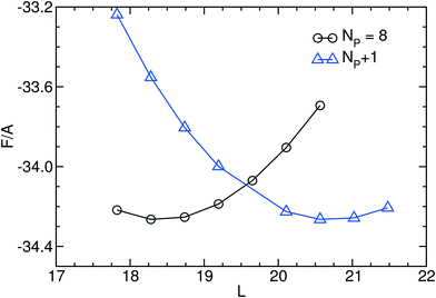
In Fig. 9 we investigate the free-energy density, F/A, of defect-free lamellae as a function of the lamellar spacing. The free-energy density exhibits a minimum at L = L0 and is well described by a quadratic form. The curvature is related to the compression modulus of the lamellae. The crossing of the two curves, FNp(L)/A with Np = 8 and 8 + 1, identifies the spacing or distance, Ly = NpL, between the guiding stripes where the free-energy density of the inner, compressed, Np = 8 + 1 and outer, expanded lamellae, Np = 8, is equal and the boundary-induced compression force vanishes. For Np = 8 this cancellation of the compression force occurs at a mismatch of about 7%. If Ly increases further, the outer lamellae are less favorable than the inner ones, and the defects move as to eliminate the outer lamellae of higher free-energy density.
The consequence of a mismatch between the periodicity, Ly, of a sparse guiding pattern and the appropriate multiple of the lamellar bulk spacing on the forces between the defect cores is illustrated in Fig. 10. We present the excess free-energy, ΔFd, as a function of the distance D between the defect cores for impact parameter, Δ = L0. At not too small distance, D > 2L0, the free energy linearly increases with D. The inset of Fig. 10 presents the slope, K = −dΔFd/dD, in this linear regime of D as a function of the system size, L in the direction perpendicular to the lamellae. Clearly as the outer lamellae become stretched Ly/Np = L > L0, the free-energy difference between the inner and outer lamellae decreases and so does the compression force, K.
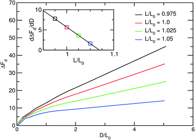 | ||
| Fig. 10 Excess free energy ΔFd of defect morphology for different values of lamellar period, L, as a function of the distance, D, between defect cores. The inset presents the slope dΔFd/dD as a function of L/L0 (cf.eqn (39)). | ||
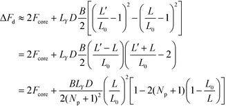
The scaling with the perpendicular system size, Ly = NpL, can be rationalized as follows: the free-energy density of the lamellae in the vicinity of the equilibrium spacing L0, can be approximated by  , where B denotes the compression modulus. Using L′ = Ly/(Np + 1) we can thus approximate the total free energy of the system by
 | (38) |
 | (39) |
This rational suggest that the compression force decreases as the number, Np of lamellae increases,  for L ≈ L0,53 and that the compression force decreases approximately linearly with L and vanishes if the lamellae are stretched to
  . This prediction is corroborated by the inset of Fig. 10, highlighting that the defect motion is very sensitive to a mismatch between the periodicity, NpL, of a sparse guiding pattern and the appropriate multiple of the lamellar bulk spacing, NpL0.
3.5 Design of device-oriented copolymer structures
Interactions between the guiding pattern and the copolymer material can be straightforwardly incorporated in continuum models by augmenting the free-energy functional by an additional surface contribution, which describes the wetting behavior71
 | (40) |
We start from a perfectly homogeneous state, m(x) ![[triple bond, length as m-dash]](https://www.rsc.org/images/entities/char_e002.gif) 0, at time, t = 0. Since our calculations ignore thermal fluctuations, the kinetics of structure formation is deterministic. Therefore our calculations highlight how the guiding fields direct the self-assembly. Similar to surface-directed spinodal decomposition72,73 in blends, different stages in the kinetics of structure formation can be distinguished:
0, at time, t = 0. Since our calculations ignore thermal fluctuations, the kinetics of structure formation is deterministic. Therefore our calculations highlight how the guiding fields direct the self-assembly. Similar to surface-directed spinodal decomposition72,73 in blends, different stages in the kinetics of structure formation can be distinguished:
1. Surface-directed spinodal self-assembly
• linear growth of composition variation driven by surface fields
• exponential amplification of composition fluctuations
2. Changes of the domain topology
In the first stage, the surface fields induce the enrichment of the preferred segment species at the location of the guiding field. Including the surface contribution and setting m(x) ![[triple bond, length as m-dash]](https://www.rsc.org/images/entities/char_e002.gif) 0, we obtain from eqn (32)
0, we obtain from eqn (32)
m(x,![[thin space (1/6-em)]](https://www.rsc.org/images/entities/char_2009.gif) t) = Δh(x)·Λt t) = Δh(x)·Λt | (41) |
| r(q) ∼ (qξ0)2[1 − (qξ0)2] + α | (42) |
Composition variations with the wave vector  grow the fastest. Thus, in the course of the surface-directed spinodal self-assembly, a lamellar structure emerges that is registered and aligned with the guiding pattern and is characterized by the periodicity
  .
.
Since the linearized form of the SCFT is the RPA, SCFT predicts the growth rate, r(q) ∼ −q2γ2(q). Fig. 2 demonstrates that the Ohta–Kawasaki model, eqn (10), provides a rather accurate approximation for the second-order vertex function. Therefore we expect that the estimate for the periodicity, λmax, of the initial lamellar structure also is accurate.
At the order–disorder transition,  , the periodicity of the spinodal structure coincides with the equilibrium lamellar spacing, L0. Upon increasing the incompatibility, however, we observe that λmax remains unaltered when measured in the natural length unit, ξ0, of the Ohta–Kawasaki model (or decreases when measured in units of Re), whereas the equilibrium lamellar spacing, L0, increases. Using the one-mode approximation that is appropriate for weak segregation, we obtain for the ratio
 | (43) |
Also within the SCFT, the ratio  decreases as we increase the incompatibility, χN. Thus, the lamellar structure that is templated by the surface-directed self-assembly differs from the equilibrium structure. For
 ![[small alpha, Greek, tilde]](https://www.rsc.org/images/entities/i_char_e0dc.gif) = 0.0172, i.e., χN ≈ 30 the ratio of length scales is about 0.5.
= 0.0172, i.e., χN ≈ 30 the ratio of length scales is about 0.5.
3.6 DSA of T-junctions
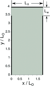
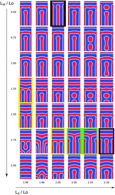
In order to illustrate the fabrication of T-junctions, we employ a two-dimensional system with reflecting boundary conditions in all directions that mimic confining walls. At the boundaries there acts a guiding field, h(x,y), according to eqn (40) that attracts the A-component with strength −0.3 or that adopts the neutral, non-preferential value 0. The system geometry is sketched in Fig. 11. The height of the system is Ly = 4L0, the top horizontal boundary attracts the A-component, whereas the bottom horizontal boundary is neutral. In the following, we aim at identifying a parameter region where the formation of the targeted structure is promoted by systematically optimizing the length, LW, of the neutral portion of the vertical side wall and the width, LX, of the confinement. The design space is restricted to the interval 1.9 ≤ LX/L0 ≤ 2.16, illustrating the role of the mismatch between the width of the confinement and the equilibrium lamellar periodicity, and . The latter quantity controls the number and location of horizontal lamellae at the top.
The final morphology, into which the dynamics converges according to eqn (32), sensitively depends on the geometry of the confinement and the guiding pattern. The outcome of the simulations of the Ohta–Kawasaki model in this two-dimensional design space are compiled in Fig. 12. The metastable structures encompass a variety of structures including T-junctions of A and B domains. Some general trends can be straightforwardly identified: (i) the larger LW is the larger is the number of horizontal lamellae at the top. Note that half an A domain of thickness L0/4 is formed at the A-attracting guiding pattern at the top. For LW/L0 ≤ 1 we often observe the formation of 1.5 horizontal A domains at the top, whereas for 1.25 ≤ LW/L0 the number of horizontal A domains increases to 2.5. (ii) For LW/L0 ≈ 0.75 and 1.75, the horizontal lamellae are rather straight because the surface pattern registers the AB interface of the lowest, horizontal A domain at a position, y, that is compatible with the equilibrium lamellar spacing. For other values of LW the lowest, horizontal A domain bulges upwards, LW/L0 = 1, or is bent downwards, LW/L0 = 1.25 and 1.5. (iii) In the range of widths, LX/L0 ≈ 2, typically half a vertical A domain forms at the left and right, A-attractive, vertical boundaries, and an additional vertical A domain is located at the center. The horizontal domains at the top and the vertical domains at the bottom join in a grain-boundary-like structure.
For a wide parameter range we observe a U-shaped B domain, formed by connecting the two neighboring, vertical B domains at the top, where they meet the horizontal lamellae.
The A domains form the desired single T-junction at the center in the rather narrow parameter regime, LW/L0 = 1.75 and 2.06 ≤ LX/L0 ≤ 2.10. The morphologies are indicated by green frames in Fig. 12. Apparently, the slightly wider system size, LX/L0 > 2, allows for the bulging at the ends of the A domains, which are located at the vertical boundaries, without pinching-off the central, vertical A-domain of the T-junction.
Another type of T-junction of A domains involves the two vertical A domains at the boundary (yellow frames in Fig. 12), and it is observed for 1.25 ≤ LW/L0 ≤ 1.5 at LX/L0 = 1.90 and 1.75 ≤ LW/L0 ≤ 2 at LX/L0 = 2.
T-junctions of B domains are fabricated at LW/L0 = 0.5 at LX/L0 = 2 and LW/L0 = 1.75 at LX/L0 = 2.16. These morphologies are indicated by black frames in Fig. 12.
At the extreme parameter values, more complex morphologies are formed. For LX/L0 ≥ 2.06 and LW/L0 ≤ 1.25 there is the possibility that the vertical A domain at the center breaks up into two circular domains and for LX/L0 ≤ 1.96 and LW/L0 ≥ 1.75 highly bent structures or morphologies with additional horizontal A domains are formed.
In Fig. 13 we illustrate the kinetics of structure formation after a quench from the disordered state, m(x) ![[triple bond, length as m-dash]](https://www.rsc.org/images/entities/char_e002.gif) 0, for the formation of a U-shaped B domain that occurs at LW = 0.75L0 and LX = 2.0L0. The evolution of self-assembly is directed by the guiding fields.
0, for the formation of a U-shaped B domain that occurs at LW = 0.75L0 and LX = 2.0L0. The evolution of self-assembly is directed by the guiding fields.
At t = 10 we observe the initial stage – surface-directed spinodal self-assembly. The guiding pattern has given rise to the formation of weakly segregated A enrichment layers at the preferential portions of the boundaries according to eqn (41). These low-amplitude composition variations are exponentially amplified by the self-assembly process in the unstable homogeneous state. This surface-directed spinodal self-assembly results in the formation of lamellar domains or order-parameter waves parallel aligned with the preferential boundaries, i.e., from the horizontal top and the two vertical sides, lamellae propagate towards the center of the system. Importantly the characteristic periodicity is set by the wavelength, λmax, of the fastest growing composition mode, cf.eqn (42), and it is significantly smaller than the equilibrium domain spacing, L0, i.e., in a system of width LX = 2L0 we observe the initial formation of 5 vertical lamellae with rather small amplitude of the order parameter.
Subsequently, at the end of the surface-directed spinodal self-assembly t = 40, the composition inside the domains attains it saturation value. Note also that the two central, vertical A domains have already merged so that only 4 vertical A domains remain – twice than in the final, metastable state at LX = 2L0.
In the later stage, t ≥ 160, the domain morphology changes as to obtain a stress-free morphology with a near-equilibrium spacing. The snapshots at t = 160, 320 and 640 illustrate that this process is rather complex, involving the merging of domains and motion of the internal AB interfaces that resembles the motion of apposing dislocation defects with impact parameter, Δ = 0 (evaporation mechanism). The details of these domain changes depend how the order-parameter waves emanating from the A-attractive boundaries interfere. This interference, in turn, is dictated by the design parameters, LW and LX. Whereas the spinodal stage lasts for 40 time units of the Ohta–Kawasaki model (using Λ = 1), the subsequent changes of the morphology take about 32 times longer.
Only at t = 1280 the final domain topology is achieved and the subsequent kinetics merely optimizes the detailed position of the internal AB interfaces. Thus, a significant fraction of the time it takes to obtain the final morphology is devoted to the changes of the domain morphology required by the mismatch of the initial periodicity, λmax, and the equilibrium domain spacing, L0. Given the use of a composition-independent Onsager coefficient, we expect that the kinetics of structure changes would be even slower if we duly accounted for the intrinsically slow “tunneling” of blocks across domains of the opposite species.54
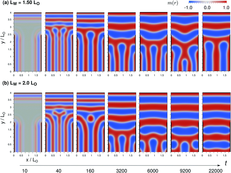
In order to illustrate the qualitative universality of the different stages and the complexity of the changes of domain topology, we investigate in Fig. 14 the case, where the width, LX = 1.9L0, is not commensurate with the equilibrium domain spacing, using two different values of LW.
For LW = 1.5L0, the surface-directed, spinodal self-assembly at the bottom is similar to Fig. 13. Short-wavelength order-parameter waves emanate from the two vertical, A-attractive guiding patterns, yielding 4 vertical A domains at the end of the spinodal self-assembly, t = 40. Since the neutral portion, LW at the top of the vertical boundaries is larger than in Fig. 13 the horizontal domain structure directed by the top boundary propagates farther downwards. Thus the transient morphology at the end of the spinodal self-assembly, t = 40, features one more horizontal A domain than in Fig. 13, and the grain boundary where the vertical and horizontal domains meet differs, resulting in an alternate sequence of domain changes in the subsequent ordering, 160 ≤ t ≤ 22![[thin space (1/6-em)]](https://www.rsc.org/images/entities/char_2009.gif) 000. Again, the domain topology changes in order to establish domains of the preferred dimension, L0. These changes involve the downward expansion of the two horizontal A domains at the top and the evaporation-like elimination of a vertical B domain at the center. The final structure consists of a T-junction of A domains that involves the two vertical A domains at the boundary. Note that the second stage – changes of the domain topology – takes about an order of magnitude longer than in the example of Fig. 13, before the final metastable morphology is attained.
000. Again, the domain topology changes in order to establish domains of the preferred dimension, L0. These changes involve the downward expansion of the two horizontal A domains at the top and the evaporation-like elimination of a vertical B domain at the center. The final structure consists of a T-junction of A domains that involves the two vertical A domains at the boundary. Note that the second stage – changes of the domain topology – takes about an order of magnitude longer than in the example of Fig. 13, before the final metastable morphology is attained.
For LW = 2L0, an additional horizontal A domain is generated by the surface-directed spinodal self-assembly at t = 40 and, concomitantly, the vertical A domains at the bottom are less extended upwards. The subsequent changes of the domain topology, involving highly curved AB interfaces, completely eliminate the vertical domains (without any barrier). Presumably, the free-energy costs of (i) slightly compressing the vertical lamellae for LX < 2L0 and of (ii) the grain boundary between vertical and horizontal domains outweigh the cost of deforming the left and right ends of the two horizontal domains in contact with the A-attractive boundaries at the lower part of the vertical boundaries. As for LW = 1.5L0, the stage of changing the domain topology is protracted.
In all these examples, most of the time is spent on the stage of changing the domain topology after the surface-directed spinodal self-assembly has templated the initial morphology. The changes of the domain topology is chiefly required because the initial morphology that is templated by the surface-directed spinodal self-assembly differs in characteristic length scale, λmax, from the domains spacing, L0, in equilibrium. Since the ratio between the two length scales differs from unity the more, the stronger the segregation strength is, cf.eqn (43), DSA at weak segregation, 10.5 < χN < 20, appears to be advantageous for rapid self-assembly directed by guiding patterns into device-oriented structures.
4 Conclusions
Continuum models have been employed to optimize parameters for the directed self-assembly (DSA) of block copolymers. By comparing the predictions of two continuum free-energy functionals – the Swift–Hohenberg model and the Ohta–Kawasaki model – to the predictions of self-consistent field theory (SCFT), we have evaluated their abilities to predict DSA-relevant properties such as the excess free energy of metastable dislocation pairs, the shape of the internal AB interfaces in the vicinity of a defect, and the kinetics of defect motion.The Swift–Hohenberg model predicts a spurious phase coexistence between a spatially modulated structure and a homogeneous structure that differs in composition.35,42 Additionally, we show that it only provides a rather poor prediction of the geometry of a prototypical, metastable defect.
The Ohta–Kawasaki model43,49,50 avoids the prediction of an unphysical macrophase separation because of the long-range 1/q2-term. We demonstrate that the model succeeds in predicting the geometry of defects as well as the transition from metastable dislocation pairs at high incompatibility to unstable ones in the vicinity of the order–disorder transition (ODT).51 Whereas the quantitative mapping from the model parameter and scales to the molecular parameters within the random-phase approximation (RPA) is only valid in the ultimate vicinity of the order–disorder transition (ODT), we have devised a phenomenological extension by adjusting the length and free-energy scales based on the comparison to SCFT. This procedure provides a reasonable agreement for equilibrium properties, including the excess free energy of dislocation-pair defects. Thus the Ohta–Kawasaki model has been proven to be a promising continuum model for studying the directed self-assembly (DSA) of diblock copolymers and design guiding patterns and geometries for device-oriented structures.
For symmetric diblock copolymers, the third-order term ![[small gamma, Greek, tilde]](https://www.rsc.org/images/entities/i_char_e0dd.gif) vanishes by symmetry, Fig. 6 suggests that the RPA-mapping,
vanishes by symmetry, Fig. 6 suggests that the RPA-mapping, ![[small alpha, Greek, tilde]](https://www.rsc.org/images/entities/i_char_e0dc.gif) (χN) in eqn (29), remains rather accurate, and the adjusted free-energy and length scales can be directly read off Fig. 3 and Fig. 4 as a function of χN. For asymmetric copolymers, to a first approximation, we expect that
(χN) in eqn (29), remains rather accurate, and the adjusted free-energy and length scales can be directly read off Fig. 3 and Fig. 4 as a function of χN. For asymmetric copolymers, to a first approximation, we expect that ![[small gamma, Greek, tilde]](https://www.rsc.org/images/entities/i_char_e0dd.gif) ∼ (2f −1) with a χN-dependent constant of proportionality. In the ultimate vicinity of the ODT,
∼ (2f −1) with a χN-dependent constant of proportionality. In the ultimate vicinity of the ODT, ![[small gamma, Greek, tilde]](https://www.rsc.org/images/entities/i_char_e0dd.gif) can be obtained from Leibler's RPA.19 For intermediate and practically relevant incompatibilities, we suggest to adjust the long-range and third-order coefficients,
can be obtained from Leibler's RPA.19 For intermediate and practically relevant incompatibilities, we suggest to adjust the long-range and third-order coefficients, ![[small alpha, Greek, tilde]](https://www.rsc.org/images/entities/i_char_e0dc.gif) (χN, f) and
(χN, f) and ![[small gamma, Greek, tilde]](https://www.rsc.org/images/entities/i_char_e0dd.gif) (χN, f), as to reproduce (i) the excess free energy of prototypical defects as in Fig. 6 and (ii) the location, flam/hex, of the transition between the lamellar and hexagonal phase predicted by SCFT.
(χN, f), as to reproduce (i) the excess free energy of prototypical defects as in Fig. 6 and (ii) the location, flam/hex, of the transition between the lamellar and hexagonal phase predicted by SCFT.
Subsequently, we have evaluated to what extent the Ohta–Kawasaki model can capture (i) the kinetics of defect motion and (ii) the surface-directed self-assembly driven by guiding patterns. The ability of the model to describe the metastability of defects and to provide insights into the kinetics of structure formation is of special relevance to DSA applications. The computational speed allows for a systematic exploration of parameter spaces – as illustrated here for a special case of a device-oriented structure. Generally, good agreement with previous SCFT calculations and particle-based simulations is obtained, apart from the following exceptions: (i) the model commonly uses a composition-independent Onsager coefficient, Λ. Computationally, this choice is very convenient for it makes the time evolution, eqn (32), local. Whereas it generally captures the qualitative features of diffusive kinetics, it grossly speeds up intrinsically slow evaporation-like events where blocks have to “tunnel” through a domain of the opposite species.54 In principle, one can account for this deficiency by using Λ ∼ ϕAϕB, imparting however, a considerable computational burden. (ii) Our study does not include thermal fluctuations. Thermal fluctuation effects can be included but, again, an accurate numerical implementation of the concomitant stochastic partial differential equation is computationally costly.74 Due to the absence of thermal fluctuations the kinetics of self-assembly cannot overcome free-energy barriers. Therefore the calculations highlight barrier-free ordering processes that are preferred for rapid and reliable DSA. (iii) The long-range kernel, G, encodes the Gaussian chain conformations. In the vicinity of impenetrable surfaces, these chain conformations are perturbed75,76 and it remains to be investigated to what extent the Ohta–Kawasaki model can account for implications of perturbed chain conformations at spatial inhomogeneities.77
In spite of these caveats, the Ohta–Kawasaki model provides valuable insights into the kinetics of self-assembly and defect motion. This model can be used in combination with more sophisticated techniques78–80 to optimize confinements suitable to fabricate device-oriented copolymer structures and limit the design space to the most promising parameter combination. Once prospective parameters for the geometry of the confinement and the guiding pattern are identified by the Ohta–Kawasaki model, more detailed simulation techniques like particle-based simulations or SCFT can be used to validate the predictions of this continuum model. This complementary use of continuum and more detailed models, enables us to gain a better understanding of the structure formation process, reducing the computational cost compared to more detailed simulation techniques.
One particularly important finding of our present study of DSA is the mismatch of the characteristic length scale of the initial surface-directed spinodal self-assembly and the equilibrium domain spacing that necessitates protracted changes of the domain morphology. This difficulty is reduced in the vicinity of the order–disorder transition, providing an additional motivation for using not too large value of the incompatibility, χN.
Conflicts of interest
There are no conflicts to declare.Acknowledgements
It is a pleasure to thank Weihua Li for fruitful and enjoyable collaboration and Ludwig Schneider, Yuliya Smirnova, and Guojie Zhang for stimulating discussions and critical comments. Financial support by the European Union FP7 under Grant agreement No. 619793 CoLiSA.MMP (Computational Lithography for Directed Self-Assembly: Materials, Models, and Processes) and the German Science Foundation Mu1764/14. We gratefully acknowledge the GWDG Göttingen, the HLRN Hannover/Berlin, and the John von Neumann Center for Computing (NIC), Jülich, Germany, for their support with ample computing time.References
- S. O. Kim, H. H. Solak, M. P. Stoykovich, N. J. Ferrier, J. J. de Pablo and P. F. Nealey, Nature, 2003, 424, 411–414 CrossRef CAS PubMed.
- J. Y. Cheng, A. M. Mayes and C. A. Ross, Nat. Mater., 2004, 3, 823–828 CrossRef CAS PubMed.
- R. A. Segalman, Mater. Sci. Eng., R, 2005, 48, 191–226 CrossRef.
- C. J. Hawker and T. P. Russell, MRS Bull., 2005, 30, 952–966 CrossRef CAS.
- M. P. Stoykovich and P. F. Nealey, Mater. Today, 2006, 9, 20–29 CrossRef CAS.
- M. P. Stoykovich, H. Kang, K. C. Daoulas, G. Liu, C. C. Liu, J. J. de Pablo, M. Müller and P. F. Nealey, ACS Nano, 2007, 1, 168–175 CrossRef CAS PubMed.
- S. B. Darling, Prog. Polym. Sci., 2007, 32, 1152–1204 CrossRef CAS.
- C. T. Black, R. Ruiz, G. Breyta, J. Y. Cheng, M. E. Colburn, K. W. Guarini, H.-C. Kim and Y. Zhang, IBM J. Res. Dev., 2007, 51, 605–633 CrossRef CAS.
- R. Ruiz, H. M. Kang, F. A. Detcheverry, E. Dobisz, D. S. Kercher, T. R. Albrecht, J. J. de Pablo and P. F. Nealey, Science, 2008, 321, 936–939 CrossRef CAS PubMed.
- I. Bita, J. K. W. Yang, Y. S. Jung, C. A. Ross, E. L. Thomas and K. K. Berggren, Science, 2008, 321, 939–943 CrossRef CAS PubMed.
- C. B. Tang, E. M. Lennon, G. H. Fredrickson, E. J. Kramer and C. J. Hawker, Science, 2008, 322, 429–432 CrossRef CAS PubMed.
- M. Luo and T. H. Epps, Macromolecules, 2013, 46, 7567–7579 CrossRef CAS.
- C. M. Bates, M. J. Maher, D. W. Janes, C. J. Ellison and C. G. Willson, Macromolecules, 2014, 47, 2–12 CrossRef CAS.
- H. Hu, M. Gopinadhan and C. O. Osuji, Soft Matter, 2014, 10, 3867–3889 RSC.
- M. A. Morris, Microelectron. Eng., 2015, 132, 207–217 CrossRef CAS.
- W. H. Li and M. Müller, Annu. Rev. Chem. Biomol. Eng., 2015, 6, 187–216 CrossRef CAS PubMed.
- W. H. Li and M. Müller, Prog. Polym. Sci., 2016, 54-55, 47–75 CrossRef CAS.
- M. Müller and J. J. de Pablo, Annu. Rev. Mater. Sci., 2013, 43, 1–34 CrossRef.
- L. Leibler, Macromolecules, 1980, 13, 1602–1617 CrossRef CAS.
- A. N. Semenov, Zh. Eksp. Teor. Fiz., 1985, 88, 1242–1256 ( Sov. Phys. JETP , 1985 , 61 , 733 ) CAS.
- P. D. Olmsted and S. T. Milner, Phys. Rev. Lett., 1994, 72, 936–939 CrossRef CAS PubMed.
- M. W. Matsen and F. S. Bates, Macromolecules, 1996, 29, 1091–1098 CrossRef CAS.
- M. W. Matsen, J. Phys.: Condens. Matter, 2002, 14, R21–R47 CrossRef CAS.
- K. C. Daoulas and M. Müller, J. Chem. Phys., 2006, 125, 184904 CrossRef PubMed.
- M. Müller, K. C. Daoulas and Y. Norizoe, Phys. Chem. Chem. Phys., 2009, 11, 2087 RSC.
- M. Müller, J. Stat. Phys., 2011, 145, 967–1016 CrossRef.
- K. C. Daoulas, M. Müller, M. P. Stoykovich, H. Kang, J. J. de Pablo and P. F. Nealey, Langmuir, 2008, 24, 1284–1295 CrossRef CAS PubMed.
- M. P. Stoykovich, K. C. Daoulas, M. Müller, H. M. Kang, J. J. de Pablo and P. F. Nealey, Macromolecules, 2010, 43, 2334–2342 CrossRef CAS.
- P. N. Patrone and G. M. Gallatin, Macromolecules, 2012, 45, 9507–9516 CrossRef CAS.
- T. Segal-Peretz, J. Ren, S. Xiong, G. Khaira, A. Bowen, L. E. Ocola, R. Divan, M. Doxastakis, N. J. Ferrier, J. de Pablo and P. F. Nealey, ACS Nano, 2017, 11, 1307–1319 CrossRef CAS PubMed.
- R. Ruiz, L. Wan, R. Lopez and T. R. Albrecht, Macromolecules, 2017, 50, 1037–1046 CrossRef CAS.
- M. Müller and K. C. Daoulas, J. Chem. Phys., 2008, 128, 024903 CrossRef PubMed.
- Z. G. Wang, J. Chem. Phys., 1994, 100, 2298–2309 CrossRef CAS.
- U. Welling, W. Li and M. Müller, SPIE Newsroom, 2014, DOI:10.1117/2.1201403.005354.
- J. Swift and P. C. Hohenberg, Phys. Rev. A: At., Mol., Opt. Phys., 1977, 15, 319–328 CrossRef.
- G. H. Fredrickson and E. Helfand, J. Chem. Phys., 1987, 87, 697–705 CrossRef CAS.
- G. H. Fredrickson and K. Binder, J. Chem. Phys., 1989, 91, 7265–7275 CrossRef CAS.
- M. Bahiana and Y. Oono, Phys. Rev. A: At., Mol., Opt. Phys., 1990, 41, 6763–6771 CrossRef CAS.
- K. R. Elder, J. Viñals and M. Grant, Phys. Rev. Lett., 1992, 68, 3024–3027 CrossRef PubMed.
- M. Seul and D. Andelman, Science, 1995, 267, 476–483 CrossRef CAS PubMed.
- Y. Tsori and D. Andelman, Europhys. Lett., 2001, 53, 722–728 CrossRef CAS.
- U. Thiele, A. J. Archer, M. J. Robbins, H. Gomez and E. Knobloch, Phys. Rev. E: Stat., Nonlinear, Soft Matter Phys., 2013, 87, 042915 CrossRef PubMed.
- T. Ohta and K. Kawasaki, Macromolecules, 1986, 19, 2621–2632 CrossRef CAS.
- F. Liu and N. Goldenfeld, Phys. Rev. A: At., Mol., Opt. Phys., 1989, 39, 4805–4810 CrossRef CAS.
- T. Ohta, Y. Enomoto, J. L. Harden and M. Doi, Macromolecules, 1993, 26, 4928–4934 CrossRef CAS.
- H. Kodama and M. Doi, Macromolecules, 1996, 29, 2652–2658 CrossRef CAS.
- S. R. Ren and I. W. Hamley, Macromolecules, 2001, 34, 116–126 CrossRef CAS.
- C. B. Muratov, Phys. Rev. E: Stat., Nonlinear, Soft Matter Phys., 2002, 66, 066108 CrossRef CAS PubMed.
- R. Choksi and X. Ren, J. Stat. Phys., 2003, 113, 151–176 CrossRef CAS.
- V. Weith, A. Krekhov and W. Zimmermann, J. Chem. Phys., 2013, 139, 054908 CrossRef PubMed.
- W. H. Li, P. F. Nealey, J. J. de Pablo and M. Müller, Phys. Rev. Lett., 2014, 113, 168301 CrossRef PubMed.
- S. M. Hur, V. Thapar, A. Ramirez-Hernandez, G. S. Khaira, T. Segal-Perez, P. A. Ricon-Delgalilio, W. Li, M. Müller, P. F. Nealey and J. J. de Pablo, Proc. Natl. Acad. Sci. U. S. A., 2015, 112, 14144 CrossRef CAS PubMed.
- W. Li and M. Müller, Macromolecules, 2016, 49, 6126–6138 CrossRef CAS.
- M. Müller and K. C. Daoulas, Phys. Rev. Lett., 2011, 107, 227801 CrossRef PubMed.
- P. Pincus, J. Chem. Phys., 1981, 75, 1996–2000 CrossRef CAS.
- P. G. de Gennes, J. Chem. Phys., 1980, 72, 4756–4763 CrossRef CAS.
- E. Reister, M. Müller and K. Binder, Phys. Rev. E: Stat., Nonlinear, Soft Matter Phys., 2001, 64, 041804 CrossRef CAS PubMed.
- P. C. Hohenberg and B. I. Halperin, Rev. Mod. Phys., 1977, 49, 435–479 CrossRef CAS.
- E. Helfand, J. Chem. Phys., 1975, 62, 999–1005 CrossRef CAS.
- J. M. H. M. Scheutjens and G. J. Fleer, J. Phys. Chem., 1979, 83, 1619–1635 CrossRef CAS.
- K. M. Hong and J. Noolandi, Macromolecules, 1981, 14, 727–736 CrossRef CAS.
- M. W. Matsen and M. Schick, Phys. Rev. Lett., 1994, 72, 2660–2663 CrossRef CAS PubMed.
- A. Arora, J. Qin, D. C. Morse, K. T. Delaney, G. H. Fredrickson, F. S. Bates and K. D. Dorfman, Macromolecules, 2016, 49, 4675–4690 CrossRef CAS.
- H. Takahashi, N. Laachi, K. T. Delaney, S.-M. Hur, C. J. Weinheimer, D. Shykind and G. H. Fredrickson, Macromolecules, 2012, 45, 6253–6265 CrossRef CAS.
- M. Müller, W. Li, J. C. Orozco Rey and U. Welling, MRS Online Proc. Libr., 2015, 1750, mrsf14-1750-kk03-05, DOI:10.1557/pol.2015.285.
- Q. Tong and S. J. Sibener, Macromolecules, 2013, 46, 8538–8544 CrossRef CAS.
- M. Peach and J. S. Koehler, Phys. Rev., 1950, 80, 436–439 CrossRef.
- M. P. Stoykovich, M. Müller, S. O. Kim, H. H. Solak, E. W. Edwards, J. J. de Pablo and P. F. Nealey, Science, 2005, 308, 1442–1446 CrossRef CAS PubMed.
- J. N. Murphy, K. D. Harris and J. M. Buriak, PLoS One, 2015, 10, 1–32 Search PubMed.
- T. Fühner, P. Michalak, U. Welling, J. C. Orozco-Rey, M. Müller and A. Erdmann, Proc. SPIE, 2016, 9780, 97800M CrossRef.
- I. Schmidt and K. Binder, J. Phys., 1985, 46, 1631–1644 CAS.
- S. Puri and K. Binder, J. Stat. Phys., 1994, 77, 145–172 CrossRef.
- P. K. Jaiswal, K. Binder and S. Puri, J. Chem. Phys., 2012, 137, 064704 CrossRef PubMed.
- J. A. de la Torre, P. Español and A. Donev, J. Chem. Phys., 2015, 142, 094115 CrossRef CAS PubMed.
- A. Silberberg, J. Colloid Interface Sci., 1982, 90, 86–91 CrossRef CAS.
- D. T. Wu, G. H. Fredrickson, J. P. Carton, A. Adjdari and L. Leibler, J. Polym. Sci., Part B: Polym. Phys., 1995, 33, 2373–2389 CrossRef CAS.
- C. Seok, K. F. Freed and I. Szleifer, J. Chem. Phys., 2004, 120, 7174–7182 CrossRef CAS PubMed.
- A. F. Hannon, Y. Ding, W. Bai, C. A. Ross and A. Alexander-Katz, Nano Lett., 2014, 14, 318–325 CrossRef CAS PubMed.
- G. S. Khaira, J. Qin, G. P. Garner, S. Xiong, L. Wan, R. Ruiz, H. M. Jaeger, P. F. Nealey and J. J. de Pablo, ACS Macro Lett., 2014, 3, 747–752 CrossRef CAS.
- S. P. Paradiso, K. T. Delaney and G. H. Fredrickson, ACS Macro Lett., 2016, 5, 972–976 CrossRef CAS.
Footnote |
| † Special collection of papers on the theme of “Advances in Directed Self-Assembly”. |
| This journal is © The Royal Society of Chemistry 2018 |

