Industrial data science – a review of machine learning applications for chemical and process industries

Abstract

In the literature, machine learning (ML) and artificial intelligence (AI) applications tend to start with examples that are irrelevant to process engineers (e.g. classification of images between cats and dogs, house pricing, types of flowers, etc.). However, process engineering principles are also based on pseudo-empirical correlations and heuristics, which are a form of ML. In this work, industrial data science fundamentals will be explained and linked with commonly-known examples in process engineering, followed by a review of industrial applications using state-of-art ML techniques.

---

Max Mowbray

Max Mowbray is a Chemical Engineering PhD student. He completed undergraduate study at the University of Birmingham, where he was fortunate to develop perspective of a wide range of research opportunities in healthcare and energy. By the end of undergraduate study, he had cultivated a desire to positively contribute to industrial transformation, which naturally led to pursuit of further study. Currently, he is undertaking postgraduate research at the University of Manchester, where he focuses on the development of data-driven methods for modelling and optimization of (bio)chemical process systems. His research extends from systems modelling to decision-making under uncertainty.

Mattia Vallerio

Mattia Vallerio graduated from Politecnico di Milano in Chemical engineering in 2010. Afterwards, He moved to Belgium where he was awarded a personal grant to persue his Ph.D. @KU Leuven in multiobjective optimization of (bio)chemical processes. After that he joined BASF Antwerp, first as APC engineer and then as advanced data analytics lead. In this role he kick-started the industrial data science field within BASF and he was at the fore-front of the site digital transformation. He recently joined Solvay as Advanced Process Control specialist. The focus of his work is on control and optimization of chemical processes.

Carlos Perez-Galvan

Carlos Perez Galvan is an industrial data scientist at Solvay in Belgium. Currently, he focuses on the solution of optimal scheduling and utility network problems using machine learning and process system engineering methods. His career in fast-moving consumer goods and manufacturing companies has lead him to develop practical expertise in the fields of modeling, simulation, optimization and machine learning. During his PhD studies at University College London, Department of Chemical Engineering (CPSE), he tackled the problem of uncertainty in nonlinear dynamic systems. He graduated from Universidad Autonoma de Coahuila in Mexico as chemical engineer in 2012.

Dongda Zhang

Dr. Dongda Zhang is a University Lecturer at the Department of Chemical Engineering, the University of Manchester, and an Honorary Research Fellow at the Centre for Process Systems Engineering, Imperial College London. He holds BSc degree (2011) from Tianjin University, MSc (Distinction) degree (2013) from Imperial College London, and PhD degree (2016) from the University of Cambridge. He currently leads research in Process Systems Engineering and Machine Learning at the Centre for Process Integration, the University of Manchester. His expertise includes developing industrially-focused data-driven and hybrid models for chemical and biochemical process simulation, optimisation and upscaling.

Antonio Del Rio Chanona

Head of the Optimisation and Machine Learning for Process Systems Engineering group at Imperial College London. Received his MEng from UNAM in Mexico, and his PhD from the University of Cambridge which received the Danckwerts-Pergamon Prize as the best doctoral thesis of his year. Received the EPSRC fellowship to adopt automation and intelligent technologies into bioprocess scaleup and industrialization and has received awards from the International Federation of Automatic Control (IFAC), and the Institution of Chemical Engineers (IChemE) in recognition for research in process systems engineering, industrialisation of bioprocesses, and adoption of intelligent and autonomous learning algorithms to chemical engineering.

Francisco J. Navarro-Brull

Industrial data scientist, Imperial College London visiting researcher, and chemical engineer working at Solvay, a Belgian company providing advanced materials and specialty chemicals worldwide. Francisco Navarro has been leading the optimization and trouble-shooting of process engineering problems using machine learning on top of advanced process control. His Ph.D. focused on the modeling and simulation of multiphase-flow sonoreactors, on which he holds two patents. He also visited Prof. Jensen Lab at MIT (USA) and co-created CAChemE.org, an open-source ChemE community based at the University of Alicante (Spain).

---

1 Introduction

The potential of data-driven applications in industrial processes has encouraged the industry to invest in machine learning teams, software, and infrastructure for the past years.^1–3 Trying to mimic big technological companies whose profit is determined by better data-driven decisions than random ones (e.g. recommending films to watch or advertisements), process industries need to deal with the safety of such recommendations in a physical setting (rather than virtual) and the inevitable challenges imposed by the physicochemical and engineering constraints.^4–6 In the same spirit of mimicking big tech companies, the IT challenge focuses on the cost, complexity, and security risk of moving process data to the cloud when in reality its majority is needed mainly locally.⁷ On the other hand, chemical companies are continuously looking at how to improve the environmental sustainability of their processes by better monitoring (maintenance) as well as yield and energy optimization. This begs the question; what are the machine learning applications that have worked so far in this Industry 4.0 revolution? What are the biggest challenges the industry is facing?

From a historical perspective, after the 1980s and 1990s, a new wave of technological innovations reflected by developments such as expert systems and neural networks promised to revolutionize the industry.⁸ Recently, applications long marked as ‘grand challenges’ have observed significant breakthroughs. For example, a solution (AlphaFold) for the task of protein structure prediction was recently proposed at CASP14, which was able to predict test protein structures with 90% accuracy. The solution could potentially provide a basis for future medical breakthroughs.⁹ Similar breakthroughs have been made in short-term weather prediction.¹⁰ Current hardware and telecommunications cost, as well as access to powerful software (either proprietary or open-source), has undoubtedly lowered the barriers to the realization of such advances. However, it is not trivial to balance the value and the cost-complexity of developing a reliable machine learning solution, which can be trusted and maintained in the long term. Thus, are these ML solutions really needed in the process industries? Or are we sometimes reinventing the wheel without knowing?

There is a common consensus in the literature^4,8,11 that addresses how:

• applying machine learning techniques without the proper process knowledge leads to correlations that can be either obvious or misleading.

• data science training for engineers can be more effective than educating data scientists in engineering topics.

The second point might be surprising, but process engineering principles were based on empirical correlations and rules-of-thumb in the past.⁴ And yet, main resources in the literature for machine learning tend to provide examples that are irrelevant to process engineers. The novelty of this review is to explain the fundamentals of machine learning with commonly-known examples in process engineering, followed by a wide range of industrial applications, from simple to state-of-art.

2 Machine learning and process systems engineering: the intuition

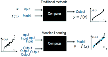
Given the high cost of generating data during the design and optimization of processes, science and engineering are built on first-principle model equations and statistical methods (e.g. design of experiments with a surface response approach¹²). In this way, initial designs can be performed with preliminary calculations for sizing, fine-tuned with first-principle simulations, and validated with a minimum number of prototypes and experiments. Contrarily, machine learning assumes having access to a vast amount of data, with enough variability, to capture all the interactions within an empirical model (Fig. 1).

Fig. 1 Contrary to the traditional approach, where first principles models are used, machine learning fits empirical models using experimental data (training data). A proper data split is necessary to introduce the right amount of model complexity and avoid overfitting.

In reality, practical applications of machine learning borrow many of the ideas used in traditional methods, as the assumption of vast and information-rich data usually falls short. For example, the hypothesis when using machine learning is to utilize the abundance of data to avoid overfitting, so that models generalize. However, as with traditional methods, the concept of parsimony, i.e., the common practice to favor simpler models (e.g. regularization and other penalized methods in machine learning), should be adopted. To better understand these similarities, let us revisit the main types of machine learning: supervised, unsupervised, and reinforcement learning.

2.1 Supervised models

If the desired output or target is known (labeled) or measured, the problem is defined as a type of categorical, discrete, or continuous regression. For instance, the estimation of heat- and mass-transfer coefficients during chemical reactor design¹³ can be seen as a supervised model that predicts the output based on a non-linear continuous fitting (see Fig. 2). Traditional pseudo-empirical correlations reduce the dimensionality of the problem to a few relevant, dimensionless variables. In machine learning, variable selection based on the variability towards the target and feature engineering can achieve the same result. Notice that the dominant physics and range of operating conditions are always given in pseudo-empirical models. The risk of extrapolation errors due to a change of the flow regime, for example, is a problem that limits the application of machine learning as well. In addition, a purely data-driven approach has the risk of overfitting when data split favors interpolation (e.g. random split), as these highly non-linear approximation functions can easily capture the noise of the training data set.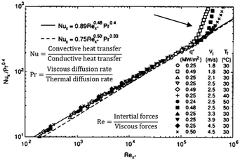

Fig. 2 Examples adapted from the literature where a non-linear model is fitted using a pseudo-empirical approach. Notice how dimensionless numbers (Re, Pr, Nu, etc.,) achieve similar results to those techniques in unsupervised machine learning, namely: feature selection, feature engineering, and dimensionality reduction. The risk of extrapolation has always been present in pseudo-empirical correlations, as models are specific to similar systems and operating conditions (the same applies to data distributions in ML). Adapted from ref. 14 with permission.

The benefits of combining machine learning with physics have proven to improve model accuracy and interpretability.¹⁵ In this context, machine learning has also been commonly applied to explain the differences between first-principle models and the real plant and the real process (a.k.a. discrepancy models).¹⁶

2.2 Unsupervised models

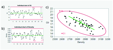
Instead of predicting a label or a measurement, the desired outcome of these models is to identify patterns or groups which remained previously unknown.

The simplest form of an unsupervised model is, for example, a control chart (see Fig. 3). In statistical process control, measurements are categorized into two groups (in-control or out-of-control) by tracking how distant they are from the statistical model. No output is required during the training/fitting, while the information (or dimensionality) is reduced from several samples to a simpler model with two statistics, in the simplest case, an average and its standard deviation. Flow maps achieved a similar goal as different fluid-dynamics patterns were discovered and grouped together via the similarity observed during experimentation.^17,18 Classical dimensionless numbers (see Fig. 2) normalize inertial, viscous, thermal- and mass-transfer magnitudes. In machine learning terminology, the use of these will be called feature selection (only relevant variables are used), feature engineering (non-linear transformations as ratios and products are calculated), and dimensionality reduction (lower number of variables to project the data and make it easier to find patterns). In this regard, data-driven techniques are being used to discover and predict flow patterns (see Fig. 4) in microfluidic applications,¹⁹ as well as turbulent and porous flows.^20,21

Fig. 3 Control charts are a form of unsupervised models where only input training data is given and a statistical model is built (mean and standard deviation). Both univariate control charts (a and b) or multivariate using principal component analysis (c) can classify data points as in or out of control.

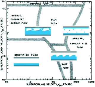Fig. 4 The discovery of flow maps where different fluid-dynamic regimes were grouped can be seen today as an unsupervised model. Adapted from ref. 17 with permission.

More generally in process engineering, dimensionality reduction naturally occurs with redundancy or excess of sensors as well. For example, if several thermocouples are used to measure a critical temperature, these can be summarized by taking the average of all the sensor readings. The average is a linear combination of all these terms with equal weight. This way, the information is being reduced to one latent variable, the temperature we want to monitor. If a big variation exists between the average of the sensors and one thermocouple, in particular, an alert can be triggered. This reasoning²² is the same behind principal component analysis (PCA), and it has been widely used for multivariate process analysis, monitoring, and control.^23–26

2.3 Reinforcement learning

Up to this point, examples given have assumed there is already data with enough variability for the purpose of estimation (model construction). However, it is often the case that a process will vary in time depending on the dynamics and control strategy implemented. For example, a PID controller is a feedback control loop that does not require any data (or model) to start (of course, the control performance will be very poor without a proper tuning of the parameters, however). Reinforcement learning (RL) is a type of machine learning method applied in the context of sequential decision-making under uncertainty (e.g. process control and optimization). As with the PID controller where the objective is to minimize the present, past, and immediate future error between the setpoint and the process variable; RL requires the definition of a reward function. Tuning the PID parameters can be done by trial and error through a combination of the user and the controller (policy), or by various tuning methods and heuristics. In RL (Fig. 5), a similar process of controller tuning is conducted through either simulation of an approximate process model, or from process data, by a set of methods known broadly as generalized policy iteration. Other heuristic approaches such as apprenticeship^27,28 and transfer learning²⁹ may also be used to identify the tuned controller.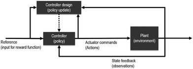

Fig. 5 Reinforcement learning can be described³⁰ as a method to tune, enhance or substitute traditional control systems.

Being a data-driven approach, RL provides more flexibility to learn non-linear, non-deterministic, more complex, and multiple input and output behaviors. The similarities between RL and advanced process control such as model predictive control or iterative learning control have been covered in the literature.^29,31,32 Despite its potential, RL is not exempt from open challenges, including guaranteeing constraints, interpretability, and safety of the operations. This is covered more in detail later in this review.

3 Industrial applications in manufacturing

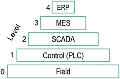
Oil and gas, chemical, and manufacturing industries store instrumentation and control data in what is known as operational historians. These time-series databases and their corresponding software collect, historize and utilize the streaming data from each sensor and actuator, which is commonly known as ‘tag’ as those physically placed to identify them at the plant level. Operational historians are usually at level 3 in the hierarchical view of automation infrastructures³³ for the ANSI/ISA-95 (see Fig. 6). Sensors and actuators in the field are operationalized by programmable logic controllers (PLC) and/or distributed control systems (DCS). Supervisory control and data acquisition (SCADA) software is often complemented with manufacturing execution systems (MES) that historized this operational data. Enterprise resource planning (ERP) data drives transactions and decisions that occur at a higher response time (months to years).³³ Machine learning takes advantage of this vast amount of historical data for the following industrial applications: condition or predictive monitoring, quality prediction, process, control optimization, and scheduling.⁶ Before implementation and industrialization, a diagnostic study is often conducted (see Fig. 7 and 8). Utilizing ML to accelerate the understanding and discovery of the root cause, which perhaps does not need a complex solution to be corrected.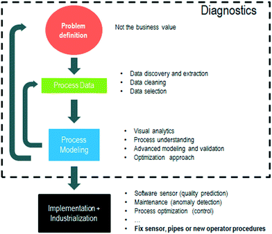

Fig. 6 Simplified hierarchical view of automation infrastructures in the standard ANSI/ISA-95.

Fig. 7 Industrial data science workflow based on the IBM cross-industry standard process for data mining (CRISP-DM).

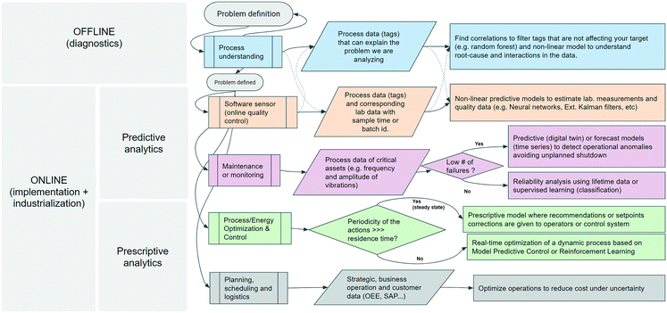Fig. 8 Classification of industrial data applications where offline analysis is commonly conducted to diagnose the problem being addressed, with the solution later implemented online.

3.1 Process understanding

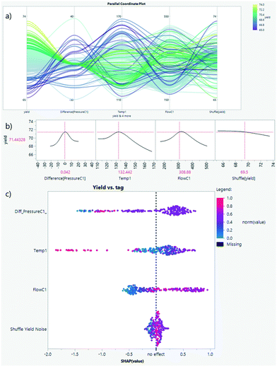
In any process or control-related problem, there will be a certain lack of information or wrong assumptions despite the amount of data stored or knowledge available. During the first phase, which can be called diagnostics, it is usually common to iterate through several data and modeling steps until the problem and potential solution are better understood. Diagnostics correspond to the beginning of any industrial application (see Fig. 7). Industrial data science can accelerate the process of discriminating what are the tags (sensors) that can help explain the problem while capturing nonlinearities via data-driven modeling techniques (see Fig. 9). The general idea is always to perform simpler, more interpretable, tree-based models for screening followed by more complex modeling techniques such as neural networks. Partition models (also known as decision trees) are common for screening, as they can handle tags with different units, the presence of missing values, and outliers while uncovering non-linear relationships. Tree-based models create simple if-then logics via data partitions that can better explain the target. As the model grows in complexity, a better fit is obtained (i.e. higher number of splits or depth in the tree). A bootstrap forest (also known as random forest³⁴) consists of several of these trees that are generated by sampling the dataset (a subset of tags and timestamps). Combining the average of the models, a more exhaustive list of potential tags (features) is obtained and ranked according to their feature importance (see Fig. 9a). However, noise within the data can be also captured. Random numbers with several types of distributions (e.g. normal, uniform…) or the target time-shuffled can be intentionally added as model parameters. This technique^35,36 is used as a cut-off and allows better separation between signal and noise, as well as the creation of simple tree models (Fig. 9b). Once the data-set is better understood and prepared, neural networks (Fig. 9c) are used to capture higher order of non-linear interactions among tags. To better illustrate common techniques in this iterative workflow, an example is provided in the annex adapting the open-source column distillation data set [Kevin Dunn, learnche.org (CC BY-SA)]. The analysis has been obtained with commercial software [JMP Pro (SAS Institute Inc.)], while all the methods are accessible via other open-source libraries [scikit learn,³⁷] as well. The working principle of these modeling techniques needs to be understood to avoid common mistakes when dealing with time-series data. For example:

Fig. 9 Common modeling steps using an industrial data set with hundreds of tags and a well-defined target (e.g. yield of the process). First, a screening of variables and selection of tags (sensors) using random forest (a). Many tags will end up being weakly correlated to the target, perhaps trying to explain its noise. By adding known noise as an additional tag(s), the selection of tags with a certain contribution is facilitated. Then, a decision tree to obtain a robust non-linear but interpretable model (b). And finally, neural networks (c) once data is cleaned and better understood to capture all the non-linearities present in the data.

• To interpret the contribution of the predictors as important towards the process design or process control. For example, the design of a reactor impeller might be critical in explaining the average quality of a product. However, if the impeller is not changed in operation, from a machine learning perspective is not important at all. Contrarily, if the current consumed by the motor was changing due to an increase/decrease of viscosity, then the current can appear as a predictor.

• Similarly, without considering the process knowledge and process dynamics, it is likely to confuse correlated effects that can be consequences instead of causes. In this regard, it is common to find measured disturbances or manipulated variables higher in the contribution. With chemical processes designed to keep critical process variables under control, inexperienced analysts will fail to interpret supervised and unsupervised analysis based on variability (e.g. the cooling flow rate in a jacketed reactor is more important than reactor temperature itself, which is always constant).

• Not managing outliers, shutdowns, and other singularities in the data. As explained above, tree-based models are robust techniques for screening predictors as they partition the data independently from its distribution. Yet, the predictors will try to explain the major sources of variability, which might be meaningless (e.g. shutdowns can be explained with pump current). The use of robust statistics using, for example, medians or interquartile ranges instead of averages and standard deviations, are a simple way to filter singular data events. However, outliers might carry crucial information as well (e.g. why the yield dropped at those specific times stamps). In this regard, gradient boosted trees are an alternative as they increase the importance of those points that could not be explained with prior models (see section 3.3.1 for more discussion).

• By default in most common algorithms, data samples are assumed to be independent of each other. This assumption can be true if each sample contains information from batch-to-batch or during steady-state conditions. In the majority of the cases, data pre-processing will be required to remove periods where time delays, dead-times, lags, and other process dynamics perturbations affect the target temporarily.³⁸ Section 3.4 will describe the applications of machine learning for dynamic systems and process control. In any case, a proper time-split of the dataset between training/validation/test is needed to decrease the risk of models that were useful in the past only (they only learned how to interpolate the data).

3.1.1 Model interpretation and explainable AI. During diagnostics, machine learning models are primarily used as screening tools to identify which inputs (tags) are affecting the target of interest. For example, support vector machines (SVM) can also be used to improve process operations similarly to decisions trees.^39,40 Pragmatically, several models with their tuning parameters can be fitted (known as autoML).^41,42 What is still relevant is: what question to ask the data, how to avoid over-fitting, and the use of Explainable AI⁴³ (data-driven techniques to interpret what more complex ML models are able to capture, see Fig. 10 as an example). For example, resampling inputs while maintaining their distribution (a.k.a. shuffling) will have a measurable impact on the prediction results. Given the non-linear interactions in the model, the interpretation of multidimensional local perturbations requires high order polynomials,⁴⁴ or even tree-based models can be used to approximate the response of a higher complex model. The latter approach, known as TreeSHAP (SHapley Additive exPlanations), has gained popularity in the ML community as it is starting to be applied in manufacturing environments.^45–48

3.2 Condition monitoring and digital twins

Often marketed as predictive maintenance, the goal is to keep critical assets working as long as possible anticipating the need for repairs (reliability increase and minimization of unplanned stops). If the assets are operated until failure and time-to-event is recorded, lifetime distributions and survival analysis can be used for prediction instead. However, the limitation when trying to apply this approach is that, fortunately, these critical assets are designed and maintained to avoid downtime failures. Therefore, a more reasonable objective is what is called anomaly detection or condition monitoring which promotes the early discovery or warning of uncommon operations. Three main methods exist.

3.2.1 Data-driven approach: statistical or machine learning. Instead of tracking time series data independently in control charts, a common step is to monitor correlated variables. What is important in this approach is to have robust dimensionality reduction, clustering, and regression methods in order to deal with potential outliers and nonlinearities that are commonly found in the data sets (e.g. planned shutdowns).

Dimensionality reduction techniques such as PCA, or PLS in case of regression, have been widely used for multivariate process analysis, monitoring, and control.^23–26 Similarly, in machine learning the basic idea is to create a model with historical data—which is assumed the normal operation—so an alert or anomaly will be triggered when something previously unseen happens. These models that learn the usual behavior of the asset are often marketed as digital twins, which, if accurate enough, can later be used for process optimization as well. From univariate control charts to parallel coordinate plots (see Fig. 10a), current technology is able to provide these visualizations in interactive dashboards which can be updated regularly or in real-time. Although classical statistical process control methods are out of the scope of this work, they should not be disregarded as a powerful way to provide descriptive statistics that can ease day-to-day decision-making in operations with little technological effort.

Fig. 10 The more traditional parallel coordinates plot (a) provides a multivariate data visualization of the distribution for different tags, which can be ordered by contribution to the model and colored by the target. In this example, pressure should be kept constant to achieve higher targeted yields (yellow vs. blue color). A machine learning model can be used to approximate and visualize the conditional relationship between yield and a given predictor (b). SHAP values (c) combine the visualization for the direction of interest (higher or lower values of the inputs in blue to magenta) but also their effect on the target. For instance, the small impact of the synthetic noise parameters (slope and SHAP value of shuffle yield in b and c, respectively).

For example, in Fig. 11 diagnostic plots for the PCA-based multivariate control chart identify a large step change in the flow of a reactant into the reactor. This affects many variables across the Tennessee Eastman process plant which are brought back to their original control limits, with the exception of the chemical A feed flow variable, where the step change was introduced (details can be found in ref. 49 and 50).

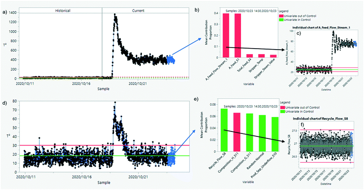Fig. 11 A transition between two steady-state regimes for the Tennessee Eastman process (simulated data⁴⁹) is detected using PCA. If the model is built using historical data before the perturbation (a) the step changes in the feed flow of chemical A (b and c) are found in the current dataset for the points highlighted in blue. If all of the historical data is used to build the model (d) the contribution of recent data points in blue (e) shows signals close to random noise. The plant wide control in the simulation stabilizes the control loops and anomalies are only seen in the transition period, even though the plant is operating in a different state for chemical A.

The addition of machine learning analysis using, for example, recent dimensionality reduction techniques, adds another layer of powerful visualizations that can enhance monitoring activities. The reader is referred to Joswiak et al.⁵¹ who recently published examples visualizing industrial chemical processes both with classical approaches (PCA and PLS) but also more recent and powerful techniques in machine learning (UMAP⁵² and HDBSCAN,^53,54 particularly). The main advantage of these state-of-art techniques is the better separation (dimensionality reduction) and classification (clustering) of events when dealing with non-stationary multivariate processes (see Fig. 12). However, if processes are under control, PCA/PLS-based techniques provide faster, less complex, and more interpretable insights (e.g. understanding variable contributions for linearized systems). Isolation forests have also been explored in order to detect and explain sources of anomalies in industrial datasets.⁵⁵

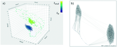Fig. 12 A transition between two steady-state regimes for the Tennessee Eastman process (simulated data⁴⁹) visualized with (a) PCA and (b) UMAP.⁵² UMAP is able to better reduce the number of tags into two dimensions. The reader is referred to ref. 51.

Autoencoders are a type of neural network (see Fig. 13) where the aim is to learn a compressed latent representation of the input in the hidden layers. The amount of information that these latent dimensions express is maximized by trying to recover the information given (notice that inputs and outputs in the neural network are the same in Fig. 13a). By restricting the neural network to a reduced number of intermediate nodes (i.e. latent dimensions), intrinsic and not necessarily linear correlations are found in order to minimize the prediction error (Fig. 13b). This way, the variability and contribution in noisy inputs will only appear if a higher number of nodes is used (similar to having a higher number of principal components). Reducing the number of redundant sensors to look at while capturing the system dynamics is a necessary step for realistic industrial data applications,^56–58 a topic we will cover in more detail later in this manuscript.

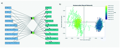Fig. 13 Similar to PCA, autoencoders are neural networks (a) that reduce the dimensionality of the data by restricting the number of nodes in the middle layers. The transition between two feeding steady-state regimes for a Tennessee Eastman process (simulated data^49,50) is captured (b) while noisy and redundant measures are discarded.

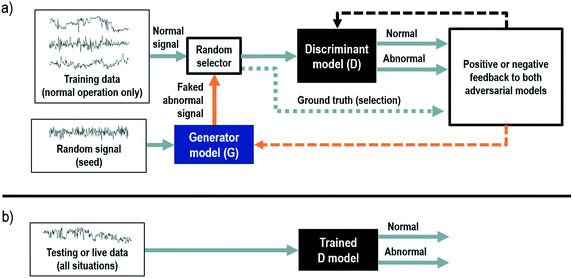
One important use of anomaly detection is to minimize the risk of extrapolation in a regression model. This is a common problem if the model is to be utilized for simulation or optimization, where the combination of input values may not be physically realizable. One approach shown in Fig. 14 is to use a regularized Hotelling T2, which can be used to find data-driven optimal values without the risk of extrapolation.^59,60 First principle, energy and mass balance can be used as additional restrictions for this regard. Finally, generative adversarial networks (GANs) represent the most recent development in the field of data-driven anomaly detection.⁶¹ GANs emerge from research in computer vision and image recognition where two competing neural networks are pitted against each other. The first network the generator (G), has the objective to capture the distribution of the input dataset (in our case process data) by identifying relevant features and generating new synthetic data. While, the other network, referred to as the discriminator (D), has the task to correctly label the presented data (i.e. original vs. generated) based on the data generated by the generator. A schematic representation of this approach for time series data can be seen in Fig. 15. See ref. 62 and 63 and references therein for early applications of GANS to time-series data.

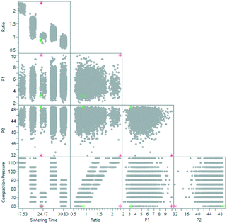Fig. 14 Scatterplot matrix showing historical data of a manufacturing process where the optimal prediction point is shown without extrapolation control (red) and with extrapolation control (green). A boosted neural network was previously trained to predict failure and quality. The reader is referred to ref. 60 for a detailed discussion.

Fig. 15 This figure shows a simplified schematic representation of training (a) and use (b) of generative adversarial networks (GANs) for anomaly detection on time-series data. Generator (G) and discriminant (D) models are trained through iterations based on the performance feedback of the D model. Both models compete until satisfactory performances are achieved. Then, D model can be used as an online classifier for anomaly detection, bottom scheme.

3.2.2 Model-driven approach. Traditionally, KPIs of critical assets are monitored by tracking their efficiency or throughput via energy or mass balances (see Fig. 16a). In machine learning terminology this is covered by the feature engineering step which can be implemented using templates for specific assets. A frequency analysis of rotary equipment, for example, can be seen as another kind of model-based approach as it provides fingerprints that are connected to the performance of rotary machines, for example (see Fig. 16b).

Fig. 16 Compressor characteristic (a) and spectrogram (b) are two traditional approaches to detect inefficient or anomaly operating modes. These calculations can be considered feature engineering to be combined with statistical or machine learning methods.

3.2.3 Network analysis approach. Process data contains sensor deviations and errors, known or unknown changes in operating modes or shutdowns, etc. which make the task of maintaining models online very challenging. Contextualizing information is crucial to minimize the number of false alerts and to increase the use of these tools for root-cause analysis.^64–68 An anomaly that propagates and diverges through the process causes a higher priority set of alarms than those created by unusual operations. Graph analysis can be used in this regard^69–71 to include the topology of the plant and the relations among operating units (see Fig. 17). This approach can cover the entire plant from anomaly operations and reduce the number of false positives. This is a similar line of thinking to the use of knowledge graphs for complex analyses, which are able to provide an integrated view of macro, meso- and microscale processes.⁷²

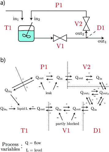Fig. 17 Process variables from a plant (a) contextualized using directed graphs (b) to reduce the number of false alerts and infer causality. Adapted with permission from ref. 70.

3.3 Quality predictive models and inferential (or soft.) sensors

In industry, quality measurements and KPIs are often manually sampled and then analyzed in the lab. Machine learning models can find process variables that correlate with such measurements, where both causes or consequences can be used to obtain an online estimation. Commonly known as inferential sensors or software sensors, one can also describe these models as semi-supervised learning since the majority of process data does not contain the target (label) to predict in the first place.

In these types of applications, a common mistake is to rapidly discard consequences from the predictor list. For example, when analyzing the quality of a granular product (good if particles are a certain size or bad if particles are smaller) one can easily find that the pressure drop in a downstream filter appears as a predictor. While this is not the root-cause of bad quality but rather a clear consequence, it can still be used for an online estimation increasing the amount of data to analyze to more than the available via lab analysis. There is this famous machine learning problem where the algorithm mistakenly learns how to classify images between huskies or wolves as a function of snow in the background.⁷³ As with the snow, consequences are often stronger or simpler predictors than perhaps other features that process experts were listing as root-causes only. For this reason, soft sensor models need to be approached separately as their main objective is to only provide online estimation and monitoring of quality, yield, and lab measurements.

As with other online sensors (e.g. NIR, near-infrared sensor), soft sensors require calibration and maintenance to ensure acceptable levels of accuracy and precision. In that regard, several techniques exist to handle prior knowledge or the lack of it (this being a form of uncertainty). An industrial example that illustrates the challenges when building soft-sensors for continuous processes can be found here.⁷⁴ Its analysis (as detailed in ref. 75) combines data preparation, anomaly detection, multivariate regression and model interpretability, so far discussed in this manuscript.

In this section, we will focus our discussion on estimating quality or yield for batch processes, which represents an additional challenge from the data analytics perspective.

3.3.1 Discrepancy models and boosting. Consider that in a production process, it is often desired to infer end-quality of the product. For example, in ref. 76, the authors discuss the merits of monitoring melt viscosity, temperature profile, and flow index as indicators of product quality in the context of polymer processing. As a result, soft sensors may be constructed to infer these qualities from other available process measurements (such as screw speed, die melt temperature, feed rates, and pressures) either via first principles, data-driven or hybrid modeling approaches.

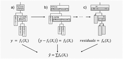
Hybrid- or grey-box models are commonly known in the literature.^77–79 A combination of data-driven models with first-principles models can remove variability or capture unknown mechanisms, e.g. discrepancy models.¹⁶ For example, if a heat or mass balance can foresee issues in quality or productivity, predictors that are part of these terms will be immediately found. Simply removing them from the input list will not change the variability on the target, so a better approach is to focus on explaining the residuals. For example, if an oscillation in the yield is found to be correlated to seasons due to better/worse cooling in winter/summer, it will be better to remove such effect from the target (not from the list of inputs) and refocus the analysis on the remaining and unexplained variability. This is what boosted tree models achieve in machine learning (see Fig. 18), and the same approach can be used in neural networks as mentioned in Fig. 14.

Fig. 18 By subsequently fitting the residuals of smaller trees, boosted trees can be used as discrepancy models where the first layers (a and b) capture the major variability within the data. Weaker but perhaps more interesting predictors can be identified by examining deep layers (c). Following the example used earlier, the first two layers are able to identify major drivers separately: a) flow and temperature; b) pressure stability.

3.3.2 Batch-to-batch or iterative models. Utilizing all the data from batch processes represents a challenge, as the model output can be one measurement (e.g. predicting quality) while model inputs range from raw materials properties to initial and evolving conditions that are or were changing during the batch. Different approaches on how to effectively reduce this apparent excess of data (dimensionality) while maintaining the information to understand, detect anomalies or use predictions for control can be found in ref. 24, 25 and 80.

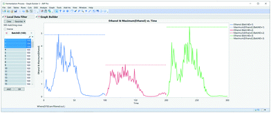
A common approach is to summarize each batch using statistics and process knowledge (peak temperature or its average rate of change during the reaction phase). In the literature, these are known as landmark points or fingerprints (see Fig. 19), but it usually assumes we know what are the important features to generate. Generalizing this approach, one can calculate common statistics (average, max, min, range, std, first, last, or their robust equivalent), for every sensor during every phase, for every batch and grade. In auto-machine learning, this is known as feature engineering so a final feature selection is made using only the best predictors. Instead of trying to summarize the information in statistical calculations that can aggregate and dilute important information, functional principal components analysis (FPCA) is a data-driven method to capture the variation between a set of “functions”, such as the profiles of temperature versus time for a set of batches. With FPCA, the functions are decomposed into the mean function and a series of “eigenfunctions” or functional principal components (FPCs). Each original function can be reconstituted as a combination of the mean function plus some amount of each functional principal component. The first step is to turn the semi-continuous data of the sensor value at each timepoint for each batch into a continuous function. This is done by fitting smoothing models, such as splines, to create continuous functions. This means it is possible to use both dense (observations are on the same equally spaced grid of time points for all batches) and sparse (batches have different numbers of observations and are unequally spaced over time) functional data. Then a functional principal components analysis is carried out. FPCA is analogous to standard PCA in that it seeks to reduce the data into a smaller number of components describing as much information in the data as possible. FPCA finds a set of component functions that explain the maximal amount of variation in the observed functions. These component functions can usually be interpreted as distinctive features that are seen in the process for some batches (see Fig. 20). For example, a temperature “spike” at a certain point in the process, or a “shoulder” in the cool-down part of the process. Finally, the results from the FPCA, especially the FPC scores, are saved and used as features for further analysis. The FPC scores can be thought of as the “amount” of each characteristic functional component that there is in each function (batch).

Fig. 19 Model inputs for batch processes can be generated by summarizing the information, which is known as landmark points in the literature. Here, the maximum temperature reached during fermentation can be found to be correlated to the quality of the batch.

Fig. 20 Functional PCA summarizes the batch information into new coordinate variables that capture variability seen during the batch. In the image, batch curves can be described again using a combination of components 1 and 2.

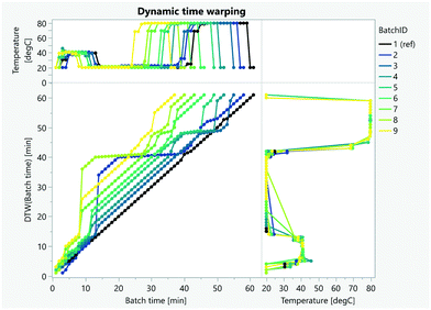
FPCA requires the alignment of batches to remove variability in the time axis. Some reaction phases can take longer due to different kinetics or simply waiting times due to scheduling decisions. On some occasions, using conversion instead of time will automatically align the batches. When this information or other variables such as automation triggers⁸¹ are not measured or unknown, dynamic time warping techniques (DTW) can be used to statistically align the batch trajectories (Fig. 21).^80,82,282 DTW can also be used to classify anomalous batches and to identify correlating parameters (Fig. 22).^82–86

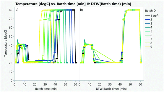Fig. 21 Alignment of several batches using the temperature profile and dynamic time warping (a before and b after the alignment).

Fig. 22 A comparison between the (original) batch time vs. time dynamically warped shows the rate at which the batches are progressing relative to the reference (batchID 1). In this illustrative example, batches are getting shorter so the rate is always positive.

3.3.2.1 Iterative learning control. Generally, the model construction process and estimation of uncertainty are subject to a finite amount of data, which can lead to over- or under-estimation. Sampling and bootstrap techniques (see next section) can be used to handle such a scenario and this is often useful in the estimation of the underlying distribution of data empirically. Various iterative-learning (control) methods also exist that help to adapt model estimates (or control inputs) when the model is used to predict the ongoing process.^87,88 The inference of these batch properties can be used to inform process operation as well as optimization and control.⁸⁹

3.3.3 Uncertainty. As demonstrated, data-driven models allow process engineers to screen and identify correlated or anomalous tags. However, the construction of a model is naturally subject to sources of uncertainty that can change over time. Despite the sources of uncertainty, often we are able to construct models that capture the underlying physics of the process in the domain of interest. For example,⁷⁶ reports many examples of data-driven and first principle models, in the context of polymer processing, that are able to successfully predict the desired property (e.g. melt viscosity, temperature profile, and flow index). More widely, this is primarily due to well-established statistical practices, as encompassed by data reconciliation and validation approaches,^90,91 model selection, validation tools,⁹² data assimilation practice,^93,94 and the field of estimation theory (which is generally concerned with identifying models of systems from data).^95,96

In the following, we discuss data-driven techniques to briefly illustrate a general approach to reduce redundant tags with similar effect size, quantify the historical variability or uncertainty, to provide insight into possible future process conditions.

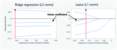
3.3.3.1 Effect size, variable, and model selection. Data-driven models are, by definition, determined by the selection of inputs and outputs. In the previous section, synthetic noise inputs were intentionally used as additional variables to find and remove those tags which showed a similar contribution towards the target.^35,36 The idea behind is that the model starts using noise as a predictor once overfitting has been reached. Another similar approach known as dropout⁹⁷ consists in removing model parameters during training, which will also take care of redundant sensors that will appear as co-linear factors in screening models. Alternatively, one can fit predictive models by penalizing the weights (if the model is parametric) of pre-selected predictors, as well as the weights of their interactions with other variables (e.g. as expressed in high order polynomials). In machine learning and statistical estimation, this penalization is also called model regularization. Two of the best-known methods of model regularization are Lasso regression,⁹⁸ where the sum of the absolute value of each of the weights (known as the L1 norm) is penalized; and the second is ridge regression,⁹⁹ which penalizes the sum of the squares of all elements of the weight vector (known as the L2 norm) (Fig. 23). Other penalization formulas using a variety of norms or their combination also exist (e.g. elastic net¹⁰⁰).

Fig. 23 Regularization is a technique that avoids over-fitting and co-linearity by penalizing a higher number and magnitude of regression terms. Ridge regression (left) penalizes the roots of squared magnitudes but is unable to remove irrelevant terms (e.g. noise) as it assumes variable selection has been done already. On the contrary, Lasso (right) minimizes absolute values being able to shrink irrelevant (e.g. noise) coefficients to zero. The red arrow line indicates the penalization parameter, increasing towards the right.

Despite the screening methods discussed that focus on identifying inputs with high correlation to outputs, the selection of model class and the associated hyperparameters also provides a basis for the identification of a strong predictive soft sensor. Current trends encompassed by AutoML⁴¹ try to automate both the identification of features and selection of models including their hyperparameter tuning. However, these frameworks are often associated with high computational expense, with further bottlenecks provided by what metric to assess and how to partition the data available. Ultimately, several optimized models need to be interpreted and verified by a domain expert (process system engineers, in this case).

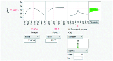
3.3.3.2 Variability in process data. Process variables (flow, pressures, etc.) are likely to observe some form of variation. This may arise from the presence of unquantified disturbances, sub-optimal control, variability in an upstream process, imperfect system measurement, etc. Assuming process variables are random variables distributed according to a distribution of choice (this can also be estimated), computational simulations (known as Monte Carlo simulation) can provide a hypothesis about the resultant effects of their variation on end-product quality. The analysis can help determine the variables with the strongest correlation to end-quality variation, which may ultimately guide process operation. This is shown in Fig. 24.

Fig. 24 Propagation of input–output uncertainties. The lack of control in pressure is simulated by including a random normal distribution in the predictive model input, generating a distribution of yield (output).

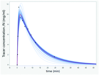
One can also augment data inputs and outputs with noisy replications of the original data to mimic process variation. This is thought to provide a form of regularization and mitigates the limits associated with small amounts of data.¹⁰¹ Such additional data can either be generated via knowledge of the physical process or statistically (via e.g. generative adversarial networks, GANs).^40,102 A similar approach to ensure robustification is to resample training and validation data in order to analyze the distribution of model outputs (see Fig. 25). Resampling techniques^103,104 also receive the name of bootstrap (as the bootstrap tree model used for screening) and include various methods (shuffling, random sampling with replacement, etc.). Such an approach acts as a form of regularization and leads to variants of well-known models, such as stochastic gradient boosted trees.¹⁰⁵

Fig. 25 Uncertainty can be estimated by resampling the data points and then analyzing the distributions of the models obtained. Here, a residence time distribution curve is generated by constructing different models subsampling data and randomly changing the importance of each point (weighted bootstrap).

All of these approaches act to robustify model construction, however, ultimately the construction process itself is always subject to finite data. As a result, cross-validation is used to assess model complexity and optimize it by evaluating the model performance using a (or numerous) validation datasets and different combinations of training and validation data (see Annex A). This reduces the risk of over-fitting to the correlation expressed in the finite amount of data and is a well-known practice within the domain of model construction.⁹²

3.3.3.3 Significance. By resampling data and ensembling the resultant models, the distribution of model parameters is obtained. If the correlations expressed in one model are not shared across the majority of the samples, a low probability of the event can be inferred (see Fig. 26). This approach follows the same ideas behind hypothesis testing,^104,106,107 and is a common problem in manufacturing where rare or temporal events are often no longer present in recent data.

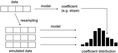Fig. 26 Uncertainty can be estimated by comparing a model (or sample statistic) with its simulated distribution using resampling techniques. For example, the slope obtained in a linear model can be compared to a distribution of the same parameter that was generated by resampling the training data. Adapted from ref. 107 with permission.

3.3.3.4 Uncertainty aware data-driven modeling. The expression of uncertainty can be captured via a model that predicts a distribution directly. As described above, the first example of this is the use of a combination of models that are created by resampling the training data; the ensemble of models that are created are then used to provide a bootstrap estimate of the uncertainty.^40,108 This has been demonstrated in ANN,¹⁰⁹ hybrid approaches,¹¹⁰ and random forest models (see annex),¹⁰⁸ amongst others.

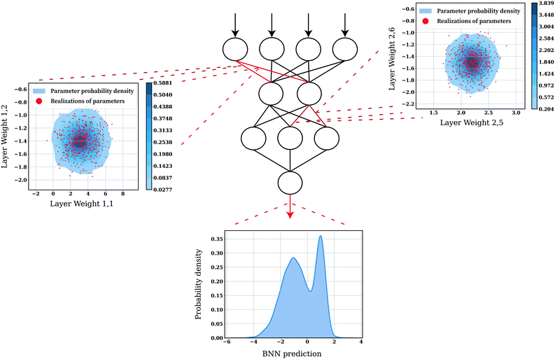
Another approach to training ANNs is provided by the Bayesian learning paradigm. Bayesian neural networks (BNN) share the same topology as conventional neural networks, but instead of having point estimates for parameters, they instead have a distribution over parameters (Fig. 27). Treating the network parameters as random variables then allows for the generation of a predictive distribution (given a model input) via the Monte Carlo method. Similarly, Bayesian extensions to other models such as support vector machines (SVMs)¹¹¹ exist.

Fig. 27 Figurative description of the Bayesian approach to express modeling uncertainty in neural networks. The top two subplots show the covariance between two-parameter distributions in the first and second layers of the network, respectively. The bottom subplot demonstrates the generation of a predictive distribution by Monte Carlo sampling the parametric distributions identified via approximate Bayesian inference.

One eloquent approach is to identify a predictive model that expresses both a nominal and uncertainty prediction in closed form.^108,112 However, unlike the Bayesian paradigm, this approach produces an uncertainty estimate of the underlying data (i.e. the natural variance of the underlying data-generating process, otherwise known as aleatoric uncertainty¹¹³) and is not reflective of the uncertainty arising from the lack of information (or data, otherwise known as epistemic uncertainty¹¹⁴) used to train the model.

Gaussian processes (GPs) are non-parametric models, which means that the model structure is not apriori-defined. This provides a highly flexible model class as GPs enable the information expressed by the model to grow as more data is acquired. In GPs, given a model input, one can directly construct a predictive distribution (i.e. a distribution over target variables) analytically via Bayesian inference and exploitation of the statistical relationships between datapoints. Further the uncertainty estimate of a GP expresses both aleatoric and epistemic uncertainty. The latter is reducible upon receipt of more data, but the former element is irreducible. This is expressed by Fig. 28.

Fig. 28 Expression of a Gaussian process posterior (i.e. its mean and uncertainty predictions) for the modeling of a smooth noiseless function. The figure demonstrates the effects of an increasing number of data points: a) 5 data points, b) 6 data points, c) 7 data points. Note how as the number of data points increases, the uncertainty estimate (i.e. the 95% confidence interval) reduces and the mean GP prediction becomes a better estimate of the ground truth.

In the scope of practical use, it should be noted the computational complexity of GPs grows cubically with the number of datapoints, so they either become intractable with large datasets or require the use of approximate Bayesian inference (as performed in variational GPs). For more detailed information on the mathematics underlying GPs, we direct to,¹¹⁵ and for an introductory tutorial, we recommend.¹¹⁶

3.4 Process control and process optimization

Despite functioning in narrow operational regions, process dynamics need to be considered if the aim is to use predictive models for control applications that are not maintained strictly at steady-state conditions (i.e. main flows and levels are fairly stable^38,117,118).

System inertia or residence time (in chemical engineering), response time or time constant (in process control), and autocorrelation (in time series models) are different characteristics of dynamical systems. For example, transportation delay (also known as dead-time) will hinder any conclusion done from pure correlation analysis (e.g. upstream changes affecting the target hours or days later). In addition, applications of machine learning modifying operation parameters need to monitor the presence or creation of plant-wide oscillations given close-loop process control or the presence of recycling streams.^119,120

In this section, we now explore the use of data-driven methods not only as monitoring or supervisory systems, but for their direct application in process control and optimization. In both cases, we are concerned with the identification of a dynamical system. For more specific discussion regarding state-of-the-art, data-driven derivative-free approaches to optimization, we direct the interested reader to this work.¹²¹

3.4.1 Dynamical systems modeling and system identification. A simplified problem statement for the modeling of dynamical systems is: given a dataset of process trajectories that express temporal observations of the system state variable, x, and control inputs, u; identify either a function, f_d, expressive of a mapping between system inputs and states at the current time index, t, and states at the next time index, t + 1, or a function, f_c, that describes the total derivative of the system state with respect to time, as well as a mapping descriptive of the mechanism of system observation, g. A general definition of discrete-time process evolution and observation is provided as follows:

x_t+1 = f_d(x_t, u_t) + w_t (System model) (1a)

y_t = g(x_t, u_t) + e_t (Measurement model) (1b)

where y_t is the measured variable, x_t is the real system state, w_t is additive system disturbance and e_t is typically a zero-mean Gaussian noise. An example of such a system is shown in Fig. 29, which shows a second-order system. The measured output y(t + 1) is, therefore, a function of u(t) but also the inertia of the system. This is implicit and observed through the evolution of the state variable, x(t), which in this example corresponds to the measured y(t).

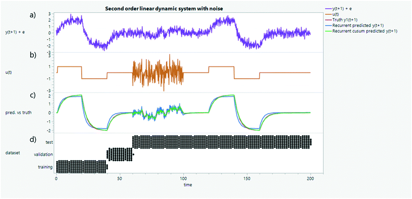Fig. 29 A second-order linear dynamical system with one (a) observed state, y(t), and (b) control input, u(t). The discrete evolution of y(t + 1) can be approximated as a function of the cumulative sum (cusum) of state (over a past horizon) and the most recent control input, instead of simply using the previous measurement. A comparison is shown in subfigure c – cusum in red vs. most recent state in green. The cusum is thought to properly account for the inertia of the system,^122,123 whereas using the most recent state produces essentially a memoryless model. Training, validation, and tests datasets are partitioned and evaluated using multi-step ahead prediction (recurrent) from an initial condition (d).

There are two primary approaches to the identification of such a function – first principles (white-box) and data-driven modeling (black-box). Generally, the benefits of first-principles approaches arise in the identification of a model structure, which is based on an understanding of the physical mechanisms driving the process. This tends to be highly useful when one would like to extrapolate away from the region of the process dynamics seen in the data. Given the remit of this paper, we focus on data-driven modeling approaches.

Particularly when interest lies in control applications, data-driven modeling of dynamical systems has been ruled by the field of system identification (SI). SI lies at the intersection of probability theory, statistical estimation theory, control theory, design of experiments, and realization theory. It follows then that the traditional ethos of SI, in the domain of PSE, constructs models that a) entail tractable parameter identification (i.e. that this estimation procedure is at the very least identifiable, but more preferably convex or analytical),¹²⁴ b) are convenient for further use in process control and optimization, and c) apply the concept of Occam's Razor.¹²⁵ As a result, this means that the models identified in classical SI are often linear in the parameters¹²⁶i.e. that process evolution can be described as a linear combination of basis functions of the system state and control input.‡ It is also worth emphasizing that such a class of models can still express nonlinearities, whilst typically gaining the ability to conduct estimation online, due to the efficiency of the algorithms available.¹²⁷ As a result, these techniques are applied not only in process industries, but also widely used in navigation and robotics.¹²⁸

Given the narrow operational region of the process industries, it has historically been dominated by the prevalence of linear time-invariant (LTI) models of dynamical systems. The general idea here is to construct the evolution of state (i.e. f_d or f_c), as well as its observation (i.e. g), as a linear combination of the current state and control input. The field of SI pioneered the efficient identification of the associated model parameters, θ_LTI, through the development of subspace identification methods.¹²⁹ One of the foundational methods provided independently by Ho and Kalman (and others) leverages the concepts of system controllability and observability to identify θ_LTI in closed form, given measurements of the system state in response to an impulse control input signal. The insight provided by this method is that the singular value decomposition (SVD) of the block Hankel matrix (composed of the output response) provides a basis decomposition equivalent to the controllability and observability matrices. This ultimately enables the identification of θ_LTIvia a solution of the normal equations – hence mitigating the requirement for gradient-based (iterative search) optimization algorithms. Clearly, a number of assumptions are required from realization theory and on the data generation process. However, a body of algorithms has been developed since to account for stochasticity¹³⁰ and other input signals.¹³¹

Given the relatively restrictive nature of LTI, innovative model structures and various modeling paradigms have been exploited in order to approximate systems (common to PSE) that exhibit nonlinear or time delay behavior. From the perspective of tackling nonlinearity, parametric and non-parametric models include (but are certainly not limited to) the Hammerstein and Wiener and their structural variants,¹³² polynomials, nonlinear autoregressive models,¹³³ and various kernel methods, such as Volterra series expansion models¹³⁴ and radial basis functions.¹³⁵ There have also been a number of methods developed to handle approximation of processes with time delay, such as first-order plus dead time (FOPDT)¹³⁶ and second-order plus dead time (SOPDT) systems¹³⁷ as well as nonlinear autoregressive moving average models with exogenous inputs (NARMAX).¹³³ Given the number and diversity of the models firmly rooted within the SI toolbox, as well as the inevitable sources of uncertainty arising in the construction of models, many of the same model validation practices are employed in SI, as were discussed in section 3.3.3.¹²⁴ With respect to parameter estimation, many algorithms have been developed to identify the associated model parameters in closed form. However, arguably, the more expressive or unconstrained the model structure becomes, the greater the dependence of parameter estimation on search-based maximum likelihood routines (otherwise known as the prediction error method (PEM) in the SI community). Perhaps the most obvious example of this is the training of neural networks, which are commonplace within the SI toolbox.¹³⁸

3.4.2 Machine learning for dynamical systems modeling. The mention of neural networks seems to have brought us full circle to the field of machine learning (ML). It is therefore a good idea to make the point that ML and SI are not so distinct as one may think. In fact, both fields are deeply rooted in statistical theory and estimation practice. Perhaps the overarching difference between traditional ML and SI is that the developments of ML are somewhat unconstrained by the concerns relevant to SI. These concerns primarily relate to the use of the models derived for the purposes of control and optimization. However, there is a certain symbiosis observed currently in the advent of many learning-based system identification¹³⁹ and control algorithms.¹⁴⁰ A particular example is provided by reinforcement learning, the general process of which can be conceptualized as simultaneous system identification and learning of control and optimization. Further discussion of reinforcement learning is provided by section 3.4.5. In the following, we outline the second (and emerging) approach to data-driven modeling of dynamical systems as provided by the field of ML.

In keeping with the previous discussion, again in the ML paradigm, one can identify either discrete dynamics f_d or continuous dynamics f_c. However, what the use of ML implies is the availability of a large, diverse, and highly flexible class of models and estimation techniques (i.e. one can select from various supervised, unsupervised, and reinforcement learning approaches). Hence, selection of a) the most appropriate model type, b) structure, c) use of features (model inputs and outputs), d) training algorithm and e) partitioning of data and model evaluation metric can only be guided by cross-validation techniques, domain knowledge and certain qualities of the data available. In some sense, this prevents the admittance of general recommendations. However, in the following paragraphs, we explore some ideas as gathered from experience.

• Selection of model type: clearly, for certain systems, a given model class will be more effective at modeling the associated dynamics than others. For example, if the system observes smooth, lipshitz continuous behavior (e.g. as is generally the case if no phase transition is present in the process), and we are interested in identifying discrete dynamics f_d, then the use of neural networks¹⁴¹ and Gaussian processes¹⁴² are particularly appealing, primarily because of the existing proofs pertaining to the universal approximation theorem, which considers continuous functions. If the data expresses discontinuities (as would be the case if generated from a process observing phase transitions), then perhaps the use of decision tree-based models would be more effective (as these models can be conceptualized as a weighted combination of step functions – although it should be noted that e.g. random forest models are often poor at generalizing predictions for the very same reason). Similarly, if the process dynamics are nonstationary, then perhaps the use of e.g. deep Gaussian processes¹⁴³ would be more desirable, given the inability of single Gaussian processes to express nonstationary dynamics (given selection of a stationary covariance function). Alternatively, one could retain the use of GPs but instead consider the use of either input or output warping, which has been shown to remedy issues caused by non-stationarity among other features of the data available.^144,145 Various other extensions for GPs also exist.¹⁴⁶ If one would like to express continuous dynamics f_c, then two approaches could be considered. Either, one could predict the parameters of a mechanistic or first principles model conditional to different points in the input space (i.e. construct a hybrid model), using a neural network, Gaussian process, etc.;⁷⁹ or one could take the approach provided by neural ordinary differential equations (neural ODE) models,¹⁴⁷ which directly learn the total derivative of the system. Despite the suitability of a given model class to a given dynamical system, innovative algorithms can be conceptualized to handle the perceived weakness of a given model class to the problem at hand. For example, returning to the problem of nonstationary dynamics, one could conceivably partition the input space and switch between a number of Gaussian process models (with stationary covariance functions) depending on the current state of the system.¹⁴⁸

• Selection of model structure: the choice of model structure pertains to decisions regarding the hyperparameters of a given model. For example, in polynomial models, the identification of higher-order terms describes the effects of interaction between input variables (i.e. enables the expression of nonlinear behavior). Similar considerations also apply when choosing activation functions in neural networks. Such a problem is not trivial and even under the choice of the correct (parametric) model class, the predictive performance is often largely dependent on the quality of structure selection. At a high level, such a problem is negated in the setting of non-parametric models, or more specifically in the case of Gaussian processes. However, consideration is still required in the appropriate selection of a covariance function. This has led to the development of automated algorithmic frameworks, as demonstrated by algorithms such as sparse identification of nonlinear dynamics (SINDy),¹⁴⁹ ALAMO¹⁵⁰ and various hyperparameter optimization frameworks.⁴¹

• Selection of features: it is important to emphasize the use of feature selection (relating both to the input and output of the model). Perhaps the most important feature selection (in relation to the model input) is the determination of those process variables which have physical relationships to those states we are interested in predicting the evolution of. This is enabled both by operational knowledge as well as building decision tree-based models on the data available and then conducting further analysis to identify important process variables.⁹² Further, even in systems that are assumed to be Markovian (i.e. where the dynamics are governed purely by the current state of the system and not by the past sequence of states), it is often the case that predictive capabilities are enhanced by the inclusion of system states at a window of previous time indices or incremental changes in the state. Intuitively, such an approach provides more information to the model. A similar idea exists in the use of a cumulative sum of past states over a horizon.^122,123 Similarly, in the context of output feature selection and predicting discrete dynamics f_d, one could construct a model, f_Δ, to estimate the discrete increment in states between time indices (such that x_t+1 = x_t + f_Δ(x_t, u_t)), which strikes similarities to the (explicit) Euler method. It is thought that the comparative advantage of such a scheme (over x_t+1 = f_d(x_t, u_t)), is that information provided from the previous state is maximised. Recent work has developed this philosophy further via a Runge–Kutta (RK) and implicit trapezoidal (IT) scheme,¹⁵¹ demonstrating both schemes are able to well predict stiff systems (with the IT scheme performing better, as one would expect).

• Selection of training algorithm: primarily quantifies the means of parameter estimation, i.e. the optimization algorithm, and (extensions too) the statistical estimation framework used to formulate the inverse problem.¹⁵² Definition of the former typically considers the dimensionality of the parameter space, as well as the nonlinearity and differentiability of the model itself. Meanwhile, the latter is governed by the decision to operate within either a Bayesian or frequentist framework (e.g. see discussion in uncertainty appendix), which subsequently gives rise to an appropriate loss function for estimation (e.g. MSE). Further decisions regarding the addition of regularization terms into the loss function may also be considered. Recent works in the domain of physics-informed deep learning, aim to extend the traditional bias-variance analysis to regularise predictions to satisfy known differential equations.¹⁵³ This appears a promising approach to incorporate physical information into ML models beyond traditional hybrid modeling approaches, however, it is generally not known how well these approaches perform when assumptions regarding the system's behavior are inaccurate (i.e. depart from ideal behavior). The selection of a statistical estimation framework also has implications for the expression of various model uncertainties as discussed previously in section 3.3.3.4. Clearly, uncertainties are important to consider (and propagate) in the (multi-step ahead) prediction of dynamical systems. Secondary to the points discussed, the training algorithm should also consider the ultimate purpose of the model. For example if we are looking to make predictions for ‘multiple-steps’ or many time indices ahead (e.g. predicting x_t+3 = f_d(f_d(f_d(x_t))) from some initial state, x_t), one should consider how the training algorithm can account for this (see ref. 154), as it is an extension of the previous problem of identifying discrete dynamics. This can also be approached by considering the selection of model structure and features (e.g. directly predicting multiple steps ahead).

• Selection of data partition and model evaluation metric: the blueprint for model training (i.e. training, validation, and testing⁹²) necessitates the appropriate partitioning of data into respective sets. It is important in dynamical systems modeling that the datapoints for validation and testing are independent from those used in training. Therefore, generations of partitions by randomly subsampling a dataset is not sufficient in the case of time-series data. To expand, consider data from a batch process. One should split the data such that separate (and entire) runs constitute data in training, validation and testing. Equally, the means of evaluation¹⁵⁵ should be strictly guided by a model's intended use. Typically, in use of models for dynamical systems, we are interested in predicting ‘multiple-steps’. In such a case, it is likely that model errors will propagate through predictions. Therefore, if intended for such, quantification of the predictive accuracy of a single-step ahead is unlikely to be a sufficient metric.

In view of the extensive discussion provided on dynamical systems modeling, the discussion now turns to data-driven control and optimization of processes with a focus on plant and process operation.

3.4.3 Model predictive control. Model predictive control (MPC) is currently the benchmark scheme in the domain of advanced process control and optimization (APC). The general idea of MPC is to identify a discrete and finite sequence of control inputs that optimizes the temporal evolution of a dynamical system over a time horizon according to some objective function.¹⁵⁶ MPC is reliant upon the identification of some finite dimensional description of process evolution as a model. Various optimization schemes (such as direct single-shooting, direct multiple shooting and direct collocation¹⁵⁷) can be deployed to identify such a sequence of control inputs according to the description provided by the model. Additionally, if operational constraints are imposed upon the problem and the underlying model is a perfect description of the system, the solution identified will be (at least locally) optimal under both the dynamical model and operational constraints, given that the control solution must satisfy the Karush–Kuhn–Tucker (KKT) conditions. However, the models we identify of our processes are not perfect descriptions and often processes are influenced by various uncertainties and disturbances. MPC schemes handle this by incorporating state-feedback. This means at each discrete control interaction the MPC scheme is able to observe (measure) the current state of the system, and then (through optimization) identifies an optimal sequence of controls over a finite discrete time horizon – the first control identified within the sequence is then input to the system and the process repeated as the system evolves. This is expressed by Fig. 30, which specifically shows a receding horizon MPC, where the length of the finite discrete time horizon used in optimization is maintained as the process evolves.

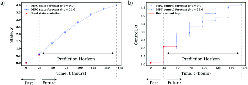Fig. 30 Demonstration of the use of state-feedback in receding horizon MPC for online optimization of an uncertain, nonlinear fed-batch process. Optimized forecast and evolution of a) the state trajectory, b) the control trajectory (composed of piecewise constant control inputs). See ref. 158 and 159 for more information on the system detailed.

To further explore the use of MPC and alternative data-driven methods with potential in the chemical process industries, we conceptualise a batch chemical process case study as outlined in ref. 160. Specifically, we are concerned with the following series reaction (catalysed by H₂SO₄) to produce some product C from a given reactant A:

where k_1A and k_2B are kinetic constants and B is an intermediate product. The reaction kinetics are first order and the compositions of A, B and C are manipulated through control of the reactor temperature via a cooling jacket and also flowrates of A into the reactor (otherwise known as control inputs, u). At specific instances in time throughout the batch, the control element is able to change the setting of these control inputs. The objective of process operation is to maximise the production of C at the end of the batch operation, with penalty for the absolute magnitude of changes in controls between each control interaction. Given that the operation is fed-batch there are a finite number of interactions the control element has available to maximize the process objective function.

In practice, we are able to identify a model describing the evolution of the underlying system composition and temperature (state, x) as a system of continuous differential equations. To deploy MPC, we can simply estimate the model parameters, discretize the model with respect to time via a given numerical method of choice and integrate it into one of the optimization schemes detailed previously. One can then optimize the process online by incorporating observation of the real system state as the process evolves and reoptimizing the control inputs over a given discrete time horizon (as displayed by Fig. 30).

There are a number of drivers within the domain of MPC research including handling nonlinear dynamics,²⁸¹ uncertainty and improving dynamical models online (or from batch to batch) using data accrued from the ongoing process.

3.4.4 Data-driven MPC. As alluded, MPC algorithms exploit various types of models, commonly developed by first principles or based on process mechanisms.¹⁶¹ Many mechanistic and empirical models are however often too complex to be used online and in addition have often high development costs. Data-driven MPC, which uses black-box identification techniques to construct its models has been exploited instead, such techniques include support vector machines,¹⁶² fuzzy models,¹⁶³ neural networks (NNs),¹⁶⁴ and Gaussian processes (GPs).¹⁶⁵ More recently, GP-based MPC algorithms that take into account online learning have been proposed.^166,167 These algorithms take information from new samples and update the existing data-driven model to account for better performance in terms of constraint satisfaction and objective function value.¹⁶⁸ Similar ideas have been taken into account in recent distributionally robust variants.¹⁶⁹

Additionally, the paradigm of MPC with learning is an MPC scheme with a nominal tracking objective and an additional learning objective.¹⁷⁰ Generally, the construction of the learning term is based on an economic optimal experiment design criterion,^170–174 furthermore, Gaussian processes have been used for optimal design of experiments.¹⁷⁵ This framework allows gathering information from the system under consideration, while at the same time optimizing it, ultimately trying to address the exploration–exploitation dilemma.

3.4.5 Reinforcement learning. The automated control of chemical processes has become paramount in today's competitive industrial setting. However, along with dynamic optimization, control is a challenging task, particularly for nonlinear and complex processes. This section introduces reinforcement learning as a tool to control and optimise chemical processes. While PID and model predictive (MPC) controllers dominate industrial practice, reinforcement learning is an attractive alternative,^29,176 as it has the potential to outperform existing techniques in a variety of applications, such as online optimization and control of batch processes.¹⁷⁷ We only discuss model-free reinforcement learning here, as model-based reinforcement learning is very closely related to data-driven MPC for chemical process applications, and a full discussion on this topic is out of the scope of this section.
3.4.5.1 Intuition. In any (discrete-time) sequential decision-making problem, there are three principal elements: an underlying system, a control element, and an objective function. The aim of the control element is to identify optimal control decisions, given observations or measurements of the underlying system. The underlying system then evolves (between control decisions) according to some dynamics. The optimality of the decisions selected by the control element and the evolution of the system is assessed by the objective function. This is a very high-level and general way to think of any decision-making process.

Under some assumptions, there is at least one sequence of decisions that is able to globally maximize a given objective function. If the evolution (or observation) of the underlying system is uncertain (stochastic), then this sequence of decisions must be reactive or conditional to the realisation of the uncertainty. In the RL paradigm, one assumes that all of the information regarding realisation of the uncertainty and current position of the system is expressed within observation or measurement of the underlying system (i.e. the state). Hence, in order to act optimally within a sequential decision making problem, the control element should be reactive to observations of state (i.e. the control element should be a control policy, π). Here we note that implementation of an MPC scheme is essentially the identification of a control policy, as realizations of process uncertainty are accounted for via state feedback as discussed in section 3.4.3.

RL describes a set of different methods capable of learning a functionalization of such a control policy, π(θ, ·), where θ are parameters of the functionalization. Further, RL does so within a closed-loop feedback control framework, independently of explicit assumptions as to the form of process uncertainty or the underlying system dynamics. This is achieved generally via sampling the underlying system with different control strategies (known as exploration) and improving the functionalization thereafter by using feedback from the system and objective function (this process is known as generalized policy iteration¹⁷⁸). An intuitive way to think about this is in terms of the design of experiments (DoE). Generally, DoE methodologies include elements that explore the design space and then subsequently exploit the knowledge that is derived from that exploration process. This process is often iterative. RL uses similar concepts but instead learns a control policy for a given sequential decision-making problem.

To further elucidate as to the benefits of RL, we now explore the conceptual fed-batch chemical process introduced in section 3.4.3. Now, assume we can estimate the uncertainties of the variables that constitute our dynamical model. If we were able to jointly express the uncertainties of the model, we could equivalently describe discrete-time dynamical evolution of the system state (i.e. reactor composition and temperature) as a conditional probability density function. In practice, we cannot express this conditional probability density function in closed form, however, we can approximate it via Monte Carlo simulation (i.e. sampling). Here lies the fundamental advantage of RL: through simulation one can express any form of uncertainty associated with a model, and through generalized policy iteration an optimal control policy for the uncertain system can be learned. This removes the requirement to identify expressions descriptive of process uncertainty in closed form (as is required in stochastic and robust variants of MPC). The use of simulation is what makes RL an incredibly general paradigm for decision making, as it enables us to consider all types of model and process uncertainties jointly. In the following, we provide intuition as to how generalized policy iteration functions.

As the uncertainty of the process is realised through simulation, at each discrete time index, t ∈ {0,…, T − 1}, process evolution is rated with respect to the process objective via a reward function, R(x_t, u_t, x_t+1). The reward function provides a scalar feedback signal, R_t+1 (that is equivalent to negative stage cost, as used in conventional controls terminology). This feedback signal can be used together with data descriptive of process evolution (i.e. {x_t, u_t, x_t+1}_t=0:T−1) via various different learning strategies to improve the policy of the control element. The general intuition of the application of RL to batch processing is provided by Fig. 31.

Fig. 31 a) A general feedback control framework for decision-making in an uncertain process. A control element interacts with an underlying system at discrete intervals in time, by changing control inputs to the system conditional to the observation of the system state. The system state then evolves in time, such that at the next time index it may be observed together with a scalar feedback signal indicative of the quality of process evolution with respect to control objectives. b) High-level intuition behind the policy optimization algorithm, REINFORCE. The system is sampled via different control strategies generated by the policy, which are exploratory and exploitative, and then the resultant data is used to improve the policy further.

Using the feedback provided by the system and the general algorithms that comprise the RL landscape, one may learn a functional parameterization of the optimal control policy for a given process. Such a parameterization is typically suited to end-to-end learning e.g. recurrent or feed-forward neural networks. There are two main families of RL algorithms, those based on (approximate) dynamic programming, and those that use policy gradients to create optimal policies. A (condensed) schematic representation of the RL algorithm landscape is shown in Fig. 32. We give an overview of these two main families of methods in the following sections below.

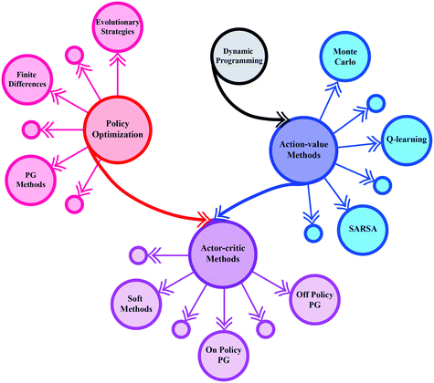Fig. 32 An overview of the RL algorithm landscape. Methods such as Q learning, which provided foundational breakthroughs for the field, are based on principles common to dynamic programming. All of these methods aim to learn the state-(action) value function. Policy optimization algorithms provide an alternative approach and specifically parameterize a policy directly. Actor-critic methods combine both approaches to enhance sample efficiency by trading-off bias and variance in learning. Figure reproduced with permission from ref. 179.

3.4.6 Reinforcement learning – dynamic programming. RL approaches based on (approximate) dynamic programming are generally termed value-based methods. This is because (for complex and continuous problems) these methods use function approximations (e.g. neural networks) to approximate the value or the action-value function. Intuitively, the value function measures how good a specific state is under a given policy, action-value methods measure how good a state-action pair is. RL algorithms use these value and value-action scores to compute optimal policies. To calculate either the value function, or the action-value function, these methods use some recursion on the Bellman equation.

Reinforcement learning, in an approximate dynamic programming (ADP) philosophy, has been explored by the chemical process control community for some time now. For example, in ref. 180 a model-based strategy and a model-free strategy for control of nonlinear processes were proposed, in ref. 181 ADP strategies were used to address fed-batch reactor optimization, in ref. 182 mixed-integer decision problems were addressed with applications to scheduling. In ref. 183 with the inclusion of distributed optimization techniques, an input-constrained optimal control problem solution technique was presented,^184,185 using Gaussian processes in this line of research, among other works (e.g. ref. 186 and 187). All these approaches rely on the (approximate) solution of the Hamilton–Jacobi–Bellman equation and have been shown to be reliable and robust for several problem instances.

Some popular value-based RL algorithms include DQN,¹⁸⁸ hindsight experience replay (HER),¹⁸⁹ distributional reinforcement learning with quantile regression (QR-DQN),¹⁹⁰ and rainbow¹⁹¹ which combines state-of-the-art improvements into DQN.

3.4.7 Reinforcement learning – policy optimization. RL algorithms based on policy optimization directly parametrize the policy by some function approximator (say a neural network), this is schematically represented in Fig. 35. Policy gradient methods are advantageous in many problem instances, and there have been many developments that have made them suitable for process optimization and control. For example, in ref. 192 the authors develop an approximate policy-based accelerated (APA) algorithm that allows the RL algorithms to converge when using more aggressive learning rates, which significantly speeds up the learning process. Further,¹⁹³ a systematic incremental learning method is presented for RL in continuous spaces where the system is dynamic, this is the case in many chemical processes, where future ambient conditions and feeds are unknown and varying, amongst other developments.^194,195

Recent research has been focusing on another side of RL for chemical process control, that of using policy gradients.^29,196 Policy gradient methods directly estimate the control policy, without the need of a model, or an online optimisation. Therefore, aside from the benefits of RL, policy gradient methods additionally exhibit the following advantages over action-value RL methods (e.g. deep Q-learning):

• Policy gradient methods enable the selection of control actions with arbitrary probabilities. In some cases (e.g. partially observable systems), the best policy may be stochastic.¹⁷⁸

• In policy gradient methods, the approximate (possibly stochastic) policy can naturally approach a deterministic policy in deterministic systems,²⁹ whereas action-value methods (that use epsilon-greedy or Boltzmann functions) select a random control action with some heuristic rule.¹⁷⁸

• Although it is possible to estimate the objective value of state-action pairs in continuous action spaces by function approximators, this does not help choose a control action. Therefore, online optimization over the action space for each time-step should be performed, which can be slow and inefficient. Policy gradient methods work directly with policies that output control actions, which is much faster and does not require an online optimization step.

• Policy gradient methods are guaranteed to converge at least to a locally optimal policy even in high dimensional continuous state and action spaces, unlike action-value methods where convergence to local optima is not guaranteed.¹⁹⁶

• In addition, policy gradients can establish a policy in a model-free fashion and excel at online computational time. This is because the online computations require only evaluation of a policy since all the computational cost is shifted offline.

The drawback of policy gradient methods is their inefficiency with respect to data, as value-based methods are much more data-efficient.

3.4.8 Reinforcement learning vs. NMPC. To demonstrate the performance of RL relative to current methods, in Fig. 33 and 34 we present one of the results from recent work.²⁹ Here, the authors employ policy optimization based RL and provide a comparison of the performance to an advanced nonlinear model predictive control (NMPC) scheme. The figures show the distribution of process trajectories (i.e. states and controls) from an uncertain, nonlinear fed-batch process. The work shows that the performance of the RL is certainly comparable to NMPC, but accounts for process uncertainty slightly better. For example, Fig. 34 shows the distribution of control trajectories generated by the two approaches. The work employs a penalty for changing controls between successive control interactions. It can be seen that the RL policy generally observes smaller changes in the controls than the NMPC. In practice, this may lead to less wear of process valves and reduce process downtime.

Fig. 33 The state trajectories generated in online optimization of an uncertain, nonlinear fed-batch biochemical process via RL and NMPC. In this case, the controller is able to observe a noisy measurement, y = [y₁, y₂], of the system state, x. Reproduced with permission from the authors.

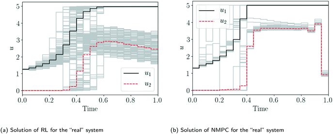Fig. 34 Comparison of the control trajectories generated via RL and NMPC in the same problem instance as in Fig. 33. The control trajectories are composed of piecewise constant control actions.

Fig. 35 A schematic representation of a framework for the application of RL to chemical process optimization. Initial policy learning is first conducted offline via simulation of an approximate process model. The policy is then transferred to the real system where it may be improved either via iterative improvement of the offline model or directly from the data accrued from process operation.

The process systems engineering community has been dealing with stochastic systems for a long time. For example, nonlinear dynamic optimization and particularly nonlinear model predictive control (NMPC) are powerful methodologies to address uncertain dynamic systems, however, there are several properties that make its application less attractive. All the approaches in NMPC require the knowledge of a detailed (and finite-dimensional) model that describes the system dynamics, and even with a detailed model, NMPC only addresses uncertainty via its finite-horizon feedback. An approach that explicitly takes into account uncertainties is stochastic NMPC (sNMPC), however, this additionally requires an assumption for the uncertainty quantification and propagation, which is difficult to estimate or even validate. Furthermore, the online computational time is a bottleneck for real-time applications since a nonlinear optimization problem has to be solved. In contrast, RL directly accounts for the effect of future uncertainty and its feedback in a proper ‘closed-loop’ manner, whereas conventional NMPC assumes open-loop control actions at future time points in the prediction, which can lead to overly conservative control actions.¹⁸⁰

3.4.9 A framework for RL in process systems engineering. Using RL directly on a process to construct an accurate controller would necessitate prohibitive amounts of data, and therefore process models must be used for the initial part of the training. This can be a detailed “knowledge-based” model, a data-driven model, or a hybrid model.²⁹

The main computational cost in RL is offline, hence in addition to the use of models, it is possible to use an existing controller to warm-start the RL algorithm to alleviate the computational burden. RL algorithms are computationally expensive in their offline stage; initially, the agent (or controller) explores the control action space randomly. In the case of process optimization and control, it is possible to use a preliminary controller, along with supervised learning or apprenticeship learning²⁸ to hot-start the policy, and significantly speed-up convergence.

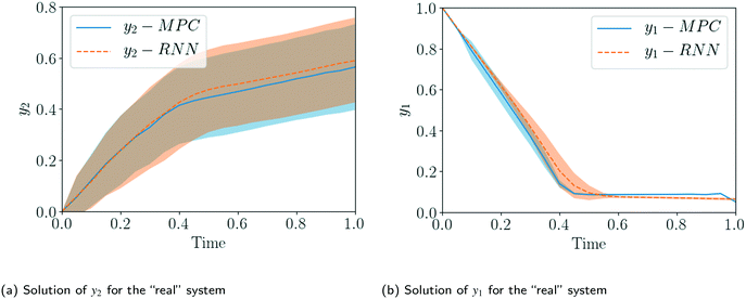
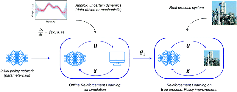
The main idea here is to have data from some policy or state-feedback control (e.g. PID controller, (economic) model predictive controller) to compute control actions given observed states. The initial parameterization for the policy is trained in a supervised learning fashion where the states are the inputs and the control actions are the outputs. Subsequently, this parameterized policy is used to initialize the policy and then trained by the RL algorithm to account for the full stochasticity of the system and avoid online numerical optimization along with the previously mentioned benefits of RL. A general methodology for conducting policy pre-training in the setting of a computational model, and then in the true system has been proposed in ref. 29, and is generally as follows:

Step 0, initialization. The algorithm is initialized by considering an initial policy network (e.g. RNN policy network) with initialized parameters (preferably by apprenticeship learning) θ₀.²⁸
Step 1, preliminary learning (offline). It is assumed that a preliminary model can be constructed from previous existing process data, hence, the policy is learned by closed-loop simulations from this model.

Given that the experiments are in silico, a large number of episodes and trajectories can be generated that corresponds to different actions from the probability distribution of u_t, and a specific set of parameters of the RNN, respectively. The resulting control policy is a good approximation of the optimal policy. Notice that if a stochastic preliminary model exists, this approach can immediately exploit it, contrary to traditional NMPC approaches. This finishes the in silico part of the algorithm, subsequent steps would be run in the true system. Therefore, emphasis after this step is given on sampling as least as possible, as every new sample results in a ‘real’ process sample.

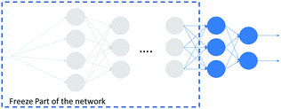
Step 2, transfer learning. The policy can now be used on a ‘real’ process, and learning can ensue by adapting all the weights from the policy network according to the policy gradient algorithm. However, this may result in undesired effects. The control policy might have a deep structure, as a result a large number of weights could be present. Thus, the optimization to update the policy may easily be stuck in a low-quality local optimum or completely diverge. To overcome this issue the concept of transfer learning is adopted, which is not exclusive of RL.¹⁹⁷ In transfer learning, a subset of training parameters is kept constant to avoid the use of a large number of epochs and episodes, applying knowledge that has been stored in a different but related problem. This technique originated from the task of image classification, where several examples exist, e.g. in ref. 198–200. See Fig. 36 for a schematic representation.

Fig. 36 Part of the network is kept frozen to adapt to new situations more efficiently.

Step 3, controlling the chemical process (online). In this step RL is applied to the chemical process by using knowledge from the model in a proper closed-loop sense and accounting for the modeled stochastic behavior (which could be from any distribution of disturbance model). Furthermore, the controller will continue to adapt and learn to better control and optimize the chemical process, addressing plant-model mismatch.¹⁵⁹

3.4.10 Real-time optimization. Real-time optimization (RTO) systems are well-accepted by industrial practitioners, with numerous successful applications reported over the last few decades.^201,202 These systems rely on knowledge-based (first principles) models, and in those processes where the optimization execution period is much longer than the closed-loop process dynamics, steady-state models are commonly employed to conduct the optimization.²⁰³ Traditionally, the model is updated in real-time using the available measurements, before repeating the optimization. This two-step RTO approach (also known as model parameter adaptation, MPA) is both intuitive and popular.

Unfortunately, although MPA is largely the most widely used RTO strategy in the industry,²⁰² it can be hindered from convergence to the actual plant optimum due to structural plant-model mismatch.^204,205 This has motivated the development of alternative adaptation schemes in RTO, such as modifier adaptation.²⁰⁶

Similar to MPA, modifier adaptation (MA) embeds the available process model into a nonlinear optimization problem that is solved at each RTO execution. The key difference is that the process measurements are now used to update the so-called modifiers that are added to the cost and constraint function in the optimization model, keeping the phenomenological model fixed at a given nominal condition. This methodology greatly alleviates the problem of offset from the actual plant optimum, by enforcing that the KKT conditions determined by the model match those of the plant upon convergence. However, this desirable property comes at the cost of having to estimate the cost and constraint gradients from process measurements.

The estimation of such plant gradients is a very difficult task to implement in practice, due to lack of information and measurement noise.^207,208 These problems have a significant effect on the gradient estimation, consequently, they reduce the overall performance of the MA scheme. Recent advances in MA schemes are reviewed in the survey paper by.²⁰⁹ Among them, there are MA-based algorithms that do not require the computation of plant derivatives. A nested MA scheme proposed by ref. 210 removes the need for estimating the plant gradients by embedding the modified optimization model into an outer problem that optimizes over the gradient modifiers using a derivative-free algorithm.²¹¹ combined MA with a quadratic surrogate trained with historical data in an algorithm called MAWQA. Likewise,²¹² investigated data-driven approaches based on quadratic surrogates.

Unfortunately, these procedures demand a series of time-consuming experimental measurements in order to evaluate the gradients of a large set of functions and variables. Given the considerable impact on productivity, these implementations are virtually absent in current industrial practice.²⁰²

3.4.11 Real-time optimization via machine learning. The main contributions of ML to RTO have been primarily directed towards improving the modifier adaptation (MA) scheme. In ref. 213, the authors augment the conventional MA scheme (i.e. using zeroth and first-order feedback from the plant) with a feedforward scheme, which provides a data-driven approach to handling non-stationarity in plant disturbances. Specifically, an ANN is constructed in order to classify the disturbance and suggest a suitable initial point for the MA scheme thereafter. The results presented in the work demonstrate impressive performance improvements when the feedforward classification structure is implemented. However, the results also detail the sensitivity of the method to low data regimes and the appropriate selection of ANN model structure.

An approach that efficiently handles low data regimes is provided by the augmentation of MA schemes with Gaussian process (GP). Here, (multiple) GPs are used to provide a mapping from control inputs to terms descriptive of mismatch in the constraints and in the objective function. This mitigates the requirement to identify zeroth and first-order terms descriptive of a mismatch from plant measurements as in the original MA scheme.²¹⁴ This approach was further extended in ref. 215, where a filtering scheme was proposed to reduce large changes in control inputs between RTO iterations; and in ref. 216, where a trust-region and Bayesian optimization were combined to balance exploration and exploitation of the GP models. Both works demonstrated good results, however, unlike the previous work of ref. 213 all of these works assume that the plant disturbance is stationary.

Another approach proposed recently deployed RL for RTO.²¹⁷ The approach was completely data-driven and did not require a description of plant dynamics. Whilst the work provided an interesting, innovative preliminary study, and performed comparably to a full information nonlinear programming (NLP) model, further work should consider the issues of training an RL policy purely from a stationary data set (with no simulated description of plant dynamics). The nature of such a training scheme has the potential to drive the plant into dangerous operational regions due to the bias of the value function used in the approach. This is discussed further in section 4 within the context of safety. In addition, merging domain knowledge (via a model) and data is generally preferred to a purely data-driven approach.

3.5 Production scheduling and supply chain

Planning and scheduling is the primary plant-wide decision-making strategy for the current process industries such as the petroleum, chemical, pharmaceutical, and biochemical industry. Optimal planning and scheduling can greatly improve process efficiency and profit, reduce raw material waste, energy and storage cost, and mitigate process operational risks. Within the context of globalization and circular economy, planning and scheduling have become increasingly challenging due to the varying demand on both product quantity and quality. Although many solution approaches have been proposed from the domain of process systems engineering, they are not often applicable for solving large-scale planning and scheduling problems due to the process complexity. Furthermore, unexpected uncertainties such as volatile customer demands, variations in process times, equipment malfunction, and fluctuations in socio-economics frequently arise in a manufacturing site, causing an intractable problem to the online decision-making of process scheduling and planning. As a result, developing a data-driven based adaptive online planning and scheduling technique is of critical importance.

3.5.1 Reinforcement learning for process scheduling and planning. Traditionally, optimal scheduling plans are made using mathematical programming methods,²¹⁸ in particular, mixed integer linear programming (MILP) if only mass flow is considered, or mixed integer nonlinear programming (MINLP) if energy utilization is also taken into account. The general procedure to calculate an optimal scheduling solution is to first construct a process-wide model by considering material balance and energy balance, with binary variables (e.g. variables that can only take a value of 0 or 1) being assigned within the process model to explore different scheduling options. Then, MILP or MINLP is performed to calculate the optimal solution. However, given a large number of scheduling alternatives and complex model structures, mathematical programming is often extremely time-consuming, thus not feasible for online scheduling.

To resolve this issue, some initial studies have been proposed since 2020 in which reinforcement learning is adopted to learn from training examples to solve the process model and to generate (approximated) optimal policies for online scheduling.^219,220 Instead of using a surrogate model, the advantage of RL is that, upon its construction, it will rapidly amend the original optimal scheduling plan whenever a new disruption occurs during the process. Based on the case study provided,²¹⁹ it is found that RL can outperform the traditional mathematical programming approach. Additionally, analysing the optimal solutions proposed by RL models, new heuristics can be discovered. Nonetheless, it is worth emphasising that using RL for online scheduling is still at its infant stage, thus more thorough investigation must be conducted before it can be actually applied to the process industry. Basic intuition for the use of RL in the domain of batch chemical production scheduling follows.

Briefly, the function of the scheduling element is to identify the sequencing of various production operations on available equipment to minimize some operational cost (that may consider resource consumption, tardiness, etc.). The sequencing of these operations may be subject to constraints that define: which operations may precede or succeed others in given equipment; limits of resources available for operation (including e.g. energy, raw material, storage etc.); and, various constraints on unit availability. At given time intervals then, the scheduling element should be able to predict the scheduling of future operations on equipment items, conditional to the current state of the plant. The state of the plant may consist of: inventory levels of raw material, intermediates and products; the amount of resource available to operation; unit availability and idling; and, the time until client orders are due (obviously dependent on problem instance). How one handles the various constraints imposed on the scheduling element is not clear, clearly there is scope to handle them through a penalty function method, however, the number of constraints imposed is often large, which often provides difficulty for the RL algorithms, as there are many discontinuities in the ‘reward landscape’. Further, there are typically many operations that a given unit can process, and given the nature of RL (i.e. using a functional parameterization of a control policy), it is not clear how best to select controls. Fig. 37 and 38 show one idea proposed in recent work²²¹ and a corresponding schedule generated for the case study detailed there.

Fig. 37 Handling control constraints innately in RL-based chemical production scheduling via identification of transformations of the control prediction through standard operating procedures (i.e. precedence and disjunctive constraints and requirements for unit cleaning). a) Augmenting the decision-making process by identifying the set of controls which satisfy the logic provided by standard operating procedure at each time index, and b) implementation of a rounding policy to ensure that RL control selection satisfies the associated logic.

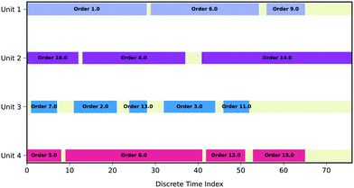Fig. 38 Solving a MILP problem via RL to produce an optimal production schedule via the framework displayed in Fig. 37. A discrete time interval is equivalent to 0.5 days in this study.

The basic idea of that work is that generally the definition of many of the constraints imposed on scheduling problems are related to control selection and governed by standard operating procedure (SOPs) (i.e. the requirement for cleaning times, the presence of precedence constraints, etc.). These SOPs essentially define logic rules, f_SOP, that govern the way in which the plant is operated and the set of operations one could schedule in units, [Doublestruck U]_t, given the current state of the plant, x_t (see Fig. 37a). As a result, one can often pre-identify the controls, which innately satisfy those constraints defined by SOPs and implement a rounding policy, f_r to alter the control predicted by the policy function to select one of those available controls (see Fig. 37b). Perhaps the largest downside of this approach is that derivative-free approaches to RL are most suitable. These algorithms are particularly suited when the effective dimensionality of the problem is low. However, the approach is known to become less efficacious when the effective dimensionality of the parameter space is large (as may be the case in the typical neural network models used in RL policy functionalization).

Clearly, the discussion provided in the latter part of this section is just one approach to handling constraints in a very particular scheduling problem instance. There is a general need for further research in the application of RL to scheduling tasks in chemical processes. This poses challenge and something both the academic and industrial communities can combine efforts in approaching. For more information, we direct the reader to a recent review.²²²

3.5.2 Reinforcement learning for supply chain optimization. The operation of supply chains is subject to inherent uncertainty as derived from market mechanisms (i.e. supply and demand),²²³ transportation, supply chain structure and the interactions that take place between organizations, and various other exogenous uncertainties (such as global weather and humanitarian events).²²⁴

Due to the large uncertainties that exist within supply chains, there is an effort to ensure that organizational behavior is more cohesive and coordinated with other operators within the chain. For example, graph neural networks (GNNs)^226,227 have been applied to help infer hidden relationships or behaviors within existing networks.^228,229 Furthermore, the combination of an increasing degree of globalization and the availability of informative data sources, has led to an interest in RL as a potential approach to supply chain optimization. This is again due to the presence of a wide range of uncertainties, combined with complex supply chain dynamics, which generally provide obstacle to existing methods. The application of RL to supply chain optimization is similarly in its infant stage, however efforts such as OR-gym²³⁰ provide means for researchers to develop suitable algorithms for standard benchmark problems. Again, this area would largely benefit from greater collaboration between academia and industry. Fig. 39 shows some training results from the inventory management problem described in ref. 230 generated by different evolutionary RL approaches including particle swarm optimization (PSO),²³¹ evolutionary strategies (ES),²³² artificial bee colony (ABC)²³³ and a hybrid algorithm with a space reduction approach.²³⁴

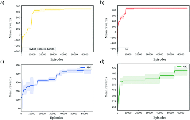Fig. 39 Solving a supply chain optimization problem via evolutionary RL methods. Reproduced with permission from ref. 225. The plots show the training process of a) a hybrid stochastic search algorithm, b) evolutionary strategies, c) particle swarm optimization, d) artificial bee colony. The algorithms demonstrate performance competitive with state-of-the-art RL approaches.

4 Challenges and opportunities

In this manuscript, we have covered the intuition behind machine learning techniques and their application to industrial processes, which have traditionally stored vasts amounts of manufacturing data in their operational historians.

More accessible and easier to use advanced analytical tools are evolving to the point where many data steps are or will be mostly automated, including the use of screening models via machine learning (i.e. AutoML). Therefore, process engineering expertise are and will be crucial to identify and define manufacturing problems to solve as well as interpret the solutions found through data-driven approaches. In many situations, once the root-cause of the problem is found, well-known solutions that can include new sensors and/or process control will be preferred over a complex approach difficult to maintain in the long run.

Advanced monitoring systems that notify suboptimal (or anomalous) behavior, list correlated factors, and allow engineers to interactively visualize process data will become the new standard in manufacturing environments. Historians with good quality and well-structured manufacturing data (e.g. batch) will become a competitive advantage, especially if a data ownership culture at the plant level is well-established.

Combined with process engineering and control knowledge, ML can be used for steady-state or batch-to-batch applications, where recommended set-points or recipe changes are suggested to operators/process engineers similar to expert systems or pseudo-empirical correlations learned from historical data. However, if the ambition is closed-loop (dynamic) systems, both data-driven MPC or reinforcement learning are limited by the following two challenges.

Implementation

Data-driven solutions and their dedicated infrastructures are less reliable than process control strategies and their systems (DCS). This has been put forward by many studies, but particularly the recent study²³⁵ summarises the concerns for the deployment of RL machinery into engineering applications. We quote the following: “we [the scientific community] do not understand how the parts comprising deep RL algorithms impact agent [controller] training, either separately or as a whole. This unsatisfactory understanding suggests that we should re-evaluate the inner workings of our algorithms. Indeed, the overall question motivating our work is: how do the multitude of mechanisms used in deep RL training algorithms impact agent [controller] behavior?”

Probably the two main takeaways from the aforementioned analysis are 1) heuristics and rules of thumb in the implementation of RL algorithms is of the utmost importance, and performance is very reliant on these details 2) large neural networks are limited by their interpretability and maintenance, and this should be further investigated.

Safety

The inclusion of safety or operational constraints is not straightforward. For example, existing methods for constrained reinforcement learning, often described as safe RL,^236,237 that are based on policy gradients cannot guarantee strict feasibility of the policies they output even when initialized with feasible initial policies.²³⁸ Various approaches have been proposed in the literature, where usually penalties are applied for the constraints. Such approaches can be very problematic, easily losing optimality or feasibility,²³⁹ especially in the case of a fixed penalty. The main approaches to incorporate constraints in this way make use of trust-region and fixed penalties,^239,240 as well as cross entropy.²³⁸ As observed in ref. 239, when penalty methods are applied in policy optimization, depending on the value of the penalty parameter the behaviour of the policy may change. If a large value of the penalty parameter is used, then the policy tends to be over-conservative resulting in feasible areas that are not optimal; on the other hand, when the value for the penalty parameter is too small, the policy tends to ignore the constraints as in the unconstrained optimization case.

5 Computational tools for data-driven modeling, control, and optimization

In this section, we provide signpost to some of the favorite computational tools of the Process Systems Engineering and Machine Learning group, University of Manchester and the Optimisation and Machine Learning for Process Systems Engineering group, Imperial College London for select model and problem classes (see Table 1). Clearly, this list is not exhaustive, but we hope it is of use to those interested in a wide range of PSE applications, who can also benefit from a glossary explaining common marching learning terms (see Table 2).

Table 1 Computational tools used by the authors and colleagues for data-driven modeling, control, and optimization in Python and Julia. This list is not exhaustive

Modeling
Model class	Python packages	Julia packages
Differential equations	SciPy^245	SciML^246
Neural ODEs	torchdiffeq,^247 JAX^248	DiffEqFlux^249
Support vector machines	Scikit-learn^37	Julia statistics – SVM
Decision tree models	Scikit-learn	DecisionTree
Gaussian processes	GPy,^250 GPyTorch,^251 GPflow^252	AbstractGPs
Artificial neural networks	PyTorch,^253 Keras,^254 JAX	Flux,^255 Knet^256
Latent variable methods	Scikit-learn, SciPy, UMAP^257	MultivariateStats,^258 UMAP
Explainable AI	SHAP,^259 LIME^260	ShapML^261
Classical Sys. ID	SciPy, SysIdentPy^262	Controlsystemidentification

---

Optimization^a
Problem class	Python packages	Julia packages
a Generally we detail packages that interface with well-established solvers, such as Gurobi^241 for mixed-integer problems and IPOPT^242 for nonlinear programming problems. This does not include commercial packages such as the MATLAB^243 Toolbox, which also provides options such as Aladin^244 for distributed optimization.
Linear programming	SciPy, CVXPY,^263 GEKKO^264	JuMP^265
Semidefinite programming	CVXPY	JuMP
Quadratic programming	CVXPy, GEKKO	JuMP
Nonlinear programming	SciPy, Pyomo,^266 NLOpt, GEKKO	JuMP, Optim, NLOpt
Mixed integer programming	Pyomo, GEKKO	JuMP
Bayesian optimization	GPyOpt,^267 HEBO,^145 BoTorch,^268 GPflowOpt^269	BayesianOptimization
MPC and dynamic opt.	Pyomo, CasADi,^270 GEKKO	InfiniteOpt^271,272
Automatic differentiation	JAX, CasADi	ForwardDiff,^273 zygote^274
Reinforcement learning	Ray,^275 RLlib,^276 Gym^277	ReinforcementLearning^278
AutoML	Ray Tune,^279 Optuna^280	AutoMLPipeline

---

Table 2 Annex III – glossary of terms

Term	Explanation
Anomaly detection	Identifies data points, events, and/or observations that deviate from a dataset's normal behavior
AutoML (model selection)	Systematic approach to select the best algorithm and its tuning parameters
Basis functions	Basic transformations used as building blocks to capture higher complexity in the data using simpler structures. For example, powers x that when added together from polynomials
Bayesian inference	Specifies how one should update one's beliefs (probability density function) about a random variable upon observing data (new and historical)
Bias-variance trade-off	Related to model complexity and generally analyzed on training data. If the model overfits the training data, it will capture all of the variability (variance), while simpler models will underfit having a higher overall error (bias)
Bootstrap	Resampling of the data to fit more robust models
Covariance	Similarity in terms of correlation between two variables affected by noise
Cross validation	Resampling technique mostly used when data availability is limited and to avoid overfitting. It consists of dividing the dataset into multiple different subsets. N-1 of these subsets are used to train the model, while the remaining one is used for validation. The chosen subset is changed iteratively till all subsets are used for validation
Dimensionality reduction	Techniques to reduce the number of input variables (e.g. tags) in a dataset by finding inner correlations (e.g. linear correlation of multiple sensors measuring the same process temperature)
Dynamic programming	Algorithmic technique for solving a sequential decision making problem by breaking it down into simpler subproblems using a recursive relationship, known as the Bellman equation
Dynamic time warping	Algorithm used to align and compare the similarity between two batches (or time series sequences) with different duration
	A common example is drying or reacting process, where time to finish depends on initial conditions and rate of change
Feature engineering	Generation of additional inputs (Xs) by transforming the original ones (usually tags). For example, the √pressure helps to find a linear relationship with respect to the flow rate. These calculations can be done automatically or by domain knowledge
Feature selection	Reduction of model inputs (e.g. tags) based on its contribution towards an output (e.g. yield) or identified group (e.g. normal/abnormal)
First-principle	Based on fundamental principles like physics or chemistry
Functional principal components	Algorithm similar to PCA to reduce the number of co-linear inputs with minimal loss of information. The main difference is that FPCE also takes into consideration both time and space dependencies of these inputs
Gaussian processes	Learning method for making predictions probabilistically in regression and classification problems
Generalized (model)	Achieved when the model is able to generate accurate outcome (predictions) in unseen data
Gradient boosted trees	Combination of decision trees that are built consecutively where each fits the residuals (unexplained variability)
Gradient methods	Optimization approach that iteratively updates one or more parameters using the rate of change to increase or decrease the goal (objective function)
Hyperparameter	Parameter used to tune the model or optimization process e.g., weights in a weighted sum objective function
Input/s (model)	Any variable that might be used by a model to generate predictions (as regressor or classifier, for example). These are known with various names, X, factors, independent variables, features… and correspond to sensor readings (tags) or their transformation (features)
Loss (or cost) function	Objective function that has to be minimized in a machine learning algorithm, usually the aggregated difference between predictions and reality
Machine learning	Data-driven models able to find: 1) correlations and classifications, 2) groups (clusters) or 3) best strategy for manipulated variables
	These types are known by 1) supervised, 2) unsupervised, and 3) reinforcement learning
Model input	Any variable that enters the model, also referred as features or Xs. Mostly, they correspond to sensor readings (tags) or a calculation from those (engineered features)
Monte Carlo simulation	Method used to generate different scenarios by varying one or more model parameters according to a chosen distribution, e.g. normal
Neural networks	Model that uses a composition of non-linear functions (e.g. linear with saturation, exponential…) in series so it can approximate any input/output relationship
Non linear	System in which the change of the output is not proportional to the change of the input
Output/s (model)	Variable or measurement to predict in supervised models. It is often referred to as Y, y, target, dependent variable... For example, y = f(x), where y is the output of the model
Partition the data	Creation of subsets for fitting the model (training), avoiding overfitting (validation) and comparing the final result with unseen data (test)
Piecewise linear	Technique to approximate non-linear functions into smaller intervals that can be considered linear
Policy optimization (gradient)	Used in reinforcement learning, it finds the direction (gradient) at which the actions can improve the long-term cumulative goal (reward)
Predictive control	Method that anticipates the behavior of the system, based on a model, several steps ahead so the optimal set of actions (manipulated variables) are calculated and perform in each iteration
Principal component analysis (PCA)	Dimensionality reduction technique that finds the correlation between input variables (tags or Xs), unveiling hidden (latent) variables that can be used instead of all them independently
Random forest	Learning algorithm that operates by subsampling the data and then constructing a multiple of decision trees in order to obtain a combined (ensembled) model that is more robust to data
Regularization/penalization	Mathematical method that introduces additional parameters in the objective/cost function to penalize the possibility that the fitting parameters would assume extreme values (e.g. LASSO, Ridge Regression, etc.)
Reinforcement learning (RL)	Fitting algorithm (training) that finds the best possible series of actions (policy) to maximize a goal (reward). Tuning a PID can be seen as a reinforcement learning task, for example
Resampling	Used when data availability is limited or contains minimal information. It consists of selecting several different data subsets combinations out of the collected data. This allows a more robust estimate of model parameters, estimating their uncertainty more accurately. A typical example in process engineering can be the the analysis of sporadic events like failures, start-ups or shut-down
Reward function	Goal of the learning process, used in RL to find the set of actions that maximizes it. Similar to an objective function in optimization, its definition will determine the solution found
Soft sensors	Type of model which is able to infer and construct state variables (whose measurement is technically difficult or relatively expensive, as for example a lab analysis) from variables that can be captured constantly from common instruments such as thermocouples, pressure transmitters, ph-meters, etc.
Supervised	If data contains an output or variable to predict (often called labels). Examples are regression or classification of images where its group is known beforehand
Supervised learning/model	Type of problem where the output of the system, sometimes called labels, is known in advance. For example, it can be numeric (e.g. regression y = f(x), being y the output) or categorical (e.g. logistic regression to predict if a lab sample will be in or out of specification looking at measurements of pH or temperature)
Support vector machines	Learning algorithm that identifies the best fit regressor (or classifier) considering a number of points within a threshold (margin). Classical regression or classification, will try to minimize the error between prediction and reality. A special type of variable transformation is used for its application to non-linear problems (known as the Kernel trick)
Tags	Unique identifier for an instrumentation signal, e.g., temperature at try 20 of distillation column or flow of material x to reactor y
Test (data)	Subset of data that a model does not use for its training or validation
Training (data)	It is a data set of examples used during the learning process and is used to fit the parameters. The goal is to produce a trained (fitted) model that generalizes well to new, unknown data
Tree-based models	Model that uses a series of if-then rules to generate predictions (model output) from one (decision tree) or more (random forest, boosted tree)
Unsupervised learning/model	When data does not contain the output to predict, sometimes called unlabeled data. These models can still obtain information by grouping (clustering) similar inputs by correlation or other similarities (e.g. control chart only has data inputs but a model is able to classify them as in- or out-of-control/anomaly)
Validation (data)	Subset of data used to avoid model overfitting

---

Disclaimer of liability

Authors and their institutions shall not assume any liability, for any legal reason whatsoever, including, without limitation, liability for the usability, availability, completeness, and freedom from defects of the reviewed examples as well as for related information, configuration, and performance data and any damage caused thereby.

Author contributions

Conceptualization M. M., A. D. R. C., and F. J. N. B.; data curation M. M. and F. J. N. B.; formal analysis M. M. and F. J. N. B.; investigation M. M. and F. J. N. B.; methodology M. M. and F. J. N. B.; project administration D. Z., A. D. R. C. and F. J. N. B.; resources M. M. and F. J. N. B.; software M. M., C. P. G. and F. J. N. B.; supervision D. Z., A. D. R. C., and F. J. N. B.; validation M. M., D. Z., and F. J. N. B.; visualization M. M., M. V., A. D. R. C., and F. J. N. B.; writing original draft M. M., M. V., A. D. R. C., and F. J. N. B.; writing – review editing M. M., C. P. G., M. V., D. Z, and F. J. N. B.

Conflicts of interest

There are no conflicts to declare.

Acknowledgements

The authors appreciate the support from JMP (SAS Institute Inc.) for facilitating the open access of this manuscript.

Notes and references

1. D. A. C. Beck, J. M. Carothers, V. R. Subramanian and J. Pfaendtner, Data science: Accelerating innovation and discovery in chemical engineering, AIChE J., 2016, 62, 1402–1416.
2. Industry 4.0: How to navigate digitization of the manufacturing sector, April 2015. [Online; accessed 13. Jul. 2020].
3. The potential of advanced process controls in energy and materials, Nov 2020. [Online; accessed 17. Sep. 2022].
4. P. M. Piccione, Realistic interplays between data science and chemical engineering in the first quarter of the 21st century: Facts and a vision, Chem. Eng. Res. Des., 2019, 147, 668–675.
5. N. Clarke, Analytics is not just about patterns in big data, ComputerWeekly.com, Nov 2016.
6. C. Shang and F. You, Data analytics and machine learning for smart process manufacturing: Recent advances and perspectives in the big data era, Engineering, 2019, 5(6), 1010–1016.
7. R. Carpi, A. Littmann and C. Schmitz, Chemicals manufacturing 2030 : More of the same…but different, Aug 2019. [Online; accessed 13. Jul. 2020].
8. V. Venkatasubramanian, The promise of artificial intelligence in chemical engineering: Is it here, finally?, AIChE J., 2019, 65, 466–478.
9. J. Jumper, R. Evans, A. Pritzel, T. Green, M. Figurnov, O. Ronneberger, K. Tunyasuvunakool, R. Bates, A. Žídek and A. Potapenko, et al., Highly accurate protein structure prediction with alphafold, Nature, 2021, 596(7873), 583–589.
10. S. Ravuri, K. Lenc, M. Willson, D. Kangin, R. Lam, P. Mirowski, M. Fitzsimons, M. Athanassiadou, S. Kashem and S. Madge, et al., Skillful precipitation nowcasting using deep generative models of radar, 2021, arXiv preprint arXiv:2104.00954.
11. S. J. Qin and L. H. Chiang, Advances and opportunities in machine learning for process data analytics, Comput. Chem. Eng., 2019, 126, 465–473.
12. R. Leardi, Experimental design in chemistry: A tutorial, Anal. Chim. Acta, 2009, 652, 161–172.
13. J. R. Couper, W. R. Penney, J. R. Fair and S. M. Walas, 17 - chemical reactors, in Chemical Process Equipment (Third Edition), ed. J. R. Couper, W. R. Penney, J. R. Fair and S. M. Walas, Butterworth-Heinemann, Boston, 3rd edn, 2012, pp. 591–653.
14. D. Vader, F. Incropera and R. Viskanta, Local convective heat transfer from a heated surface to an impinging, planar jet of water, Int. J. Heat Mass Transfer, 1991, 34(3), 611–623.
15. T. Bikmukhametov and J. Jäschke, Combining machine learning and process engineering physics towards enhanced accuracy and explainability of data-driven models, Comput. Chem. Eng., 2020, 138, 106834.
16. E. Bradford, L. Imsland, M. Reble and E. A. del Rio-Chanona, Hybrid gaussian process modeling applied to economic stochastic model predictive control of batch processes, in Recent Advances in Model Predictive Control, Springer, 2021, pp. 191–218.
17. J. Mandhane, G. Gregory and K. Aziz, A flow pattern map for gas–liquid flow in horizontal pipes, Int. J. Multiphase Flow, 1974, 1(4), 537–553.
18. S. Corneliussen, J.-P. Couput, E. Dahl, E. Dykesteen, K.-E. Frøysa, E. Malde, H. Moestue, P. O. Moksnes, L. Scheers and H. Tunheim, Handbook of Multiphase Flow Metering, Norwegian Society for Oil and Gas Measurement, 2015.
19. J. Zhang, S. Zhang, J. Zhang and Z. Wang, Machine Learning Model of Dimensionless Numbers to Predict Flow Patterns and Droplet Characteristics for Two-Phase Digital Flows, Appl. Sci., 2021, 11, 4251.
20. P. G. Constantine, Z. del Rosario and G. Iaccarino, Data-driven dimensional analysis: algorithms for unique and relevant dimensionless groups, 2017, arXiv:1708.04303.
21. X. Xie, W. K. Liu and Z. Gan, Data-driven discovery of dimensionless numbers and scaling laws from experimental measurements, Dec 2021. [Online; accessed 30. Jan. 2022].
22. K. Dunn, Extracting value from data, in Process Improvement Using Data, [Online; accessed 30. Jan. 2022, ch. 6.3].
23. J. F. MacGregor, H. Yu, S. García Muñoz and J. Flores-Cerrillo, Data-based latent variable methods for process analysis, monitoring and control, Comput. Chem. Eng., 2005, 29, 1217–1223.
24. S. García-Muñoz, T. Kourti and J. F. MacGregor, Model predictive monitoring for batch processes, Ind. Eng. Chem. Res., 2004, 43(18), 5929–5941.
25. S. García-Muñoz, T. Kourti, J. F. MacGregor, A. G. Mateos and G. Murphy, Troubleshooting of an industrial batch process using multivariate methods, Ind. Eng. Chem. Res., 2003, 42(15), 3592–3601.
26. F. Destro, P. Facco, S. García Muñoz, F. Bezzo and M. Barolo, A hybrid framework for process monitoring: Enhancing data-driven methodologies with state and parameter estimation, J. Process Control, 2020, 92, 333–351.
27. B. D. Ziebart, A. L. Maas, J. A. Bagnell and A. K. Dey, et al., Maximum entropy inverse reinforcement learning, in Aaai, Chicago, IL, USA, 2008, vol. 8, pp. 1433–1438.
28. M. Mowbray, R. Smith, E. A. Del Rio-Chanona and D. Zhang, Using process data to generate an optimal control policy via apprenticeship and reinforcement learning, AIChE J., 2021, e17306.
29. P. Petsagkourakis, I. O. Sandoval, E. Bradford, D. Zhang and E. A. del Rio-Chanona, Reinforcement learning for batch bioprocess optimization, Comput. Chem. Eng., 2020, 133, 106649.
30. B. Douglas, Reinforcement Learning, Dec 2021. [Online; accessed 1. Dec. 2021].
31. I. A. Udugama, C. L. Gargalo, Y. Yamashita, M. A. Taube, A. Palazoglu, B. R. Young, K. V. Gernaey, M. Kulahci and C. Bayer, The role of big data in industrial (bio)chemical process operations, Ind. Eng. Chem. Res., 2020, 59(34), 15283–15297.
32. D. Görges, Relations between model predictive control and reinforcement learning, IFAC-PapersOnLine, 20th IFAC World Congress, 2017, vol. 50, 1, pp. 4920–4928.
33. M. Foehr, J. Vollmar, A. Calà, P. Leitão, S. Karnouskos and A. W. Colombo, Engineering of Next Generation Cyber-Physical Automation System Architectures, SpringerLink, 2017, pp. 185–206.
34. L. Breiman, Random Forests, Mach. Learn., 2001, 45, 5–32.
35. Y. Wu, D. D. Boos and L. A. Stefanski, Controlling Variable Selection by the Addition of Pseudovariables, J. Am. Stat. Assoc., 2007, 102, 235–243.
36. S. Janitza, C. Strobl and A.-L. Boulesteix, An AUC-based permutation variable importance measure for random forests, BMC Bioinf., 2013, 14, 119.
37. F. Pedregosa, G. Varoquaux, A. Gramfort, V. Michel, B. Thirion, O. Grisel, M. Blondel, P. Prettenhofer, R. Weiss, V. Dubourg, J. Vanderplas, A. Passos, D. Cournapeau, M. Brucher, M. Perrot and E. Duchesnay, Scikit-learn: Machine learning in Python, J. Mach. Learn. Res., 2011, 12, 2825–2830.
38. J. D. Kelly and J. D. Hedengren, A steady-state detection (SSD) algorithm to detect non-stationary drifts in processes, J. Process Control, 2013, 23, 326–331.
39. G. T. Jemwa and C. Aldrich, Improving process operations using support vector machines and decision trees, AIChE J., 2005, 51, 526–543.
40. M. Mowbray, T. Savage, C. Wu, Z. Song, B. A. Cho, E. A. Del Rio-Chanona and D. Zhang, Machine learning for biochemical engineering: A review, Biochem. Eng. J., 2021, 108054.
41. F. Hutter, L. Kotthoff and J. Vanschoren, Automated machine learning: methods, systems, challenges, Springer Nature, 2019.
42. C. Thon, B. Finke, A. Kwade and C. Schilde, Artificial Intelligence in Process Engineering, Adv. Intell. Syst., 2021, 3, 2000261.
43. C. Molnar, Interpretable machine learning, Lulu. com, 2020.
44. JMP, Profilers: Jmp 12, https://www.jmp.com/support/help/Profilers.shtml#377608, 2021.
45. S. M. Lundberg and S.-I. Lee, A unified approach to interpreting model predictions, in Proceedings of the 31st international conference on neural information processing systems, 2017, pp. 4768–4777.
46. S. M. Lundberg, G. Erion, H. Chen, A. DeGrave, J. M. Prutkin, B. Nair, R. Katz, J. Himmelfarb, N. Bansal and S.-I. Lee, From local explanations to global understanding with explainable ai for trees, Nat. Mach. Intell., 2020, 2(1), 56–67.
47. J. Senoner, T. Netland and S. Feuerriegel, Using explainable artificial intelligence to improve process quality: Evidence from semiconductor manufacturing, Management Science, 2021, 1–20.
48. J. Wang, J. Wiens and S. Lundberg, Shapley flow: A graph-based approach to interpreting model predictions, in International Conference on Artificial Intelligence and Statistics, PMLR, 2021, pp. 721–729.
49. Fault Detection and Diagnosis of the Tennessee Eastman Process using Multivariate Control Charts (2020-US-45MP-606), Oct 2020. [Online; accessed 19. Dec. 2020].
50. J. Ash and J. Ding, Fault Detection and Diagnosis of the Tennessee Eastman Process using Multivariate Control Charts, ResearchGate, 2022.
51. M. Joswiak, Y. Peng, I. Castillo and L. H. Chiang, Dimensionality reduction for visualizing industrial chemical process data, Control Eng. Pract., 2019, 93, 104189.
52. L. McInnes, J. Healy and J. Melville, Umap: Uniform manifold approximation and projection for dimension reduction, 2020.
53. L. McInnes, J. Healy and S. Astels, hdbscan: Hierarchical density based clustering, J. Open Source Softw., 2017, 2(11), 205.
54. R. J. Campello, D. Moulavi and J. Sander, Density-based clustering based on hierarchical density estimates, in Pacific-Asia conference on knowledge discovery and data mining, Springer, 2013, pp. 160–172.
55. M. Carletti, C. Masiero, A. Beghi and G. A. Susto, Explainable machine learning in industry 4.0: Evaluating feature importance in anomaly detection to enable root cause analysis, in 2019 IEEE International Conference on Systems, Man and Cybernetics (SMC), IEEE, 2019, pp. 21–26.
56. S. J. Qin, Y. Liu and Y. Dong, Plant-wide troubleshooting and diagnosis using dynamic embedded latent feature analysis, Comput. Chem. Eng., 2021, 107392.
57. S. J. Qin, Y. Dong, Q. Zhu, J. Wang and Q. Liu, Bridging systems theory and data science: A unifying review of dynamic latent variable analytics and process monitoring, Annu. Rev. Control, 2020, 50, 29–48.
58. Q. Zhu, S. J. Qin and Y. Dong, Dynamic latent variable regression for inferential sensor modeling and monitoring, Comput. Chem. Eng., 2020, 137, 106809.
59. J. Ash, L. Lancaster and C. Gotwalt, A method for controlling extrapolation when visualizing and optimizing the prediction profiles of statistical and machine learning, Discovery Summit Europe 2021 Presentations, 2021.
60. J. Ash, L. Lancaster and C. Gotwalt, A method for controlling extrapolation when visualizing and optimizing the prediction profiles of statistical and machine learning models, 2022.
61. I. Goodfellow, J. Pouget-Abadie, M. Mirza, B. Xu, D. Warde-Farley, S. Ozair, A. Courville and Y. Bengio, Generative adversarial nets, Adv. Neural Inf. Process. Syst., 2014, 27, 2672–2680.
62. M. Nixon and S. Xu, Anomaly Detection in Process Data Using Generative Adversarial Networks (GAN), Aug 2021. [Online; accessed 1. Dec. 2021].
63. A. Geiger, D. Liu, S. Alnegheimish, A. Cuesta-Infante and K. Veeramachaneni, Tadgan: Time series anomaly detection using generative adversarial networks, arXiv, 2020, preprint, arXiv:2009.07769, https://arxiv.org/abs/2009.07769.
64. F. Yang and D. Xiao, Progress in root cause and fault propagation analysis of large-scale industrial processes, J. Control. Sci. Eng., 2012, 2012, 1–10.
65. F. Yang, S. Shah and D. Xiao, Signed directed graph based modeling and its validation from process knowledge and process data, Int. J. Appl. Math. Comput. Sci., 2012, 22, 41–53.
66. N. F. Thornhill and A. Horch, Advances and new directions in plant-wide disturbance detection and diagnosis, Control Eng. Pract., 2007, 15, 1196–1206.
67. M. Bauer and N. F. Thornhill, A practical method for identifying the propagation path of plant-wide disturbances, J. Process Control, 2008, 18, 707–719.
68. V. Venkatasubramanian, R. Rengaswamy and S. N. Kavuri, A review of process fault detection and diagnosis: Part II: Qualitative models and search strategies, Comput. Chem. Eng., 2003, 27, 313–326.
69. M. A. Kramer and B. L. Palowitch, A rule-based approach to fault diagnosis using the signed directed graph, AIChE J., 1987, 33, 1067–1078.
70. C. Palmer and P. W. H. Chung, Creating signed directed graph models for process plants, Ind. Eng. Chem. Res., 2000, 39(7), 2548–2558.
71. C. Reinartz, D. Kirchhübel, O. Ravn and M. Lind, Generation of signed directed graphs using functional models [U+204E][U+204E] this work is supported by the danish hydrocarbon research and technology centre, IFAC-PapersOnLine, 5th IFAC Conference on Intelligent Control and Automation Sciences ICONS 2019, 2019, vol. 52, 11, pp. 37–42.
72. T. Savage, J. Akroyd, S. Mosbach, N. Krdzavac, M. Hillman and M. Kraft, Universal Digital Twin – integration of national-scale energy systems and climate data, 2021, submitted for publication. Preprint available at https://como.ceb.cam.ac.uk/preprints/279/.
73. M. T. Ribeiro, S. Singh and C. Guestrin, why should i trust you?, Explaining the predictions of any classifier, 2016.
74. B. Braun, I. Castillo, M. Joswiak, Y. Peng, R. Rendall, A. Schmidt, Z. Wang, L. Chiang and B. Colegrove, Data science challenges in chemical manufacturing, IFAC preprints, 2020.
75. S. J. Qin, S. Guo, Z. Li, L. H. Chiang, I. Castillo, B. Braun and Z. Wang, Integration of process knowledge and statistical learning for the dow data challenge problem, Comput. Chem. Eng., 2021, 153, 107451.
76. C. Abeykoon, Design and applications of soft sensors in polymer processing: A review, IEEE Sens. J., 2019, 19, 2801–2813.
77. R. Oliveira, Combining first principles modelling and artificial neural networks: a general framework, Comput. Chem. Eng., 2004, 28(5), 755–766.
78. M. Von Stosch, R. Oliveira, J. Peres and S. F. de Azevedo, Hybrid semi-parametric modeling in process systems engineering: Past, present and future, Comput. Chem. Eng., 2014, 60, 86–101.
79. F. Vega, X. Zhu, T. R. Savage, P. Petsagkourakis, K. Jing and D. Zhang, Kinetic and hybrid modelling for yeast astaxanthin production under uncertainty, Biotechnol. Bioeng., 2021, 118, 4854–4866.
80. S. Wold, N. Kettaneh-Wold, J. MacGregor and K. Dunn, 2.10 - batch process modeling and mspc, in Comprehensive Chemometrics, ed. S. D. Brown, R. Tauler and B. Walczak, Elsevier, Oxford, 2009, pp. 163–197.
81. S. García-Muñoz, M. Polizzi, A. Prpich, C. Strain, A. Lalonde and V. Negron, Experiences in batch trajectory alignment for pharmaceutical process improvement through multivariate latent variable modelling, J. Process Control, 2011, 21(10), 1370–1377 , Special issue: selected papers from two joint IFAC conferences: 9th International Symposium on Dynamics and Control of Process Systems and the 11th International Symposium on Computer Applications in Biotechnology, Leuven, Belgium, July 5–9, 2010.
82. F. Zuecco, M. Cicciotti, P. Facco, F. Bezzo and M. Barolo, Backstepping methodology to troubleshoot plant-wide batch processes in data-rich industrial environments, Processes, 2021, 9(6), 1074.
83. M. Spooner, D. Kold and M. Kulahci, Harvest time prediction for batch processes, Comput. Chem. Eng., 2018, 117, 32–41.
84. M. Spooner and M. Kulahci, Monitoring batch processes with dynamic time warping and k-nearest neighbours, Chemom. Intell. Lab. Syst., 2018, 183, 102–112.
85. J. M. González-Martínez, A. Ferrer and J. A. Westerhuis, Real-time synchronization of batch trajectories for on-line multivariate statistical process control using dynamic time warping, Chemom. Intell. Lab. Syst., 2011, 105(2), 195–206.
86. M. Spooner, D. Kold and M. Kulahci, Selecting local constraint for alignment of batch process data with dynamic time warping, Chemom. Intell. Lab. Syst., 2017, 167, 161–170.
87. J. H. Lee and K. S. Lee, Iterative learning control applied to batch processes: An overview, Control Eng. Pract., 2007, 15(10), 1306–1318.
88. M. Barton, C. A. Duran-Villalobos and B. Lennox, Multivariate batch to batch optimisation of fermentation processes to improve productivity, J. Process Control, 2021, 108, 148–156.
89. D. Bonvin and G. François, Control and optimization of batch chemical processes, tech. rep., Butterworth-Heinemann, 2017.
90. J. A. Romagnoli and M. C. Sánchez, Data processing and reconciliation for chemical process operations, Elsevier, 1999.
91. J. Loyola-Fuentes, M. Jobson and R. Smith, Estimation of fouling model parameters for shell side and tube side of crude oil heat exchangers using data reconciliation and parameter estimation, Ind. Eng. Chem. Res., 2019, 58(24), 10418–10436.
92. J. Friedman, T. Hastie and R. Tibshirani, et al., The elements of statistical learning, Springer series in statistics, New York, 2001, vol. 1.
93. M. Asch, M. Bocquet and M. Nodet, Data assimilation: methods, algorithms, and applications, SIAM, 2016.
94. R. Arcucci, J. Zhu, S. Hu and Y.-K. Guo, Deep data assimilation: integrating deep learning with data assimilation, Appl. Sci., 2021, 11(3), 1114.
95. S. Arridge, P. Maass, O. Öktem and C.-B. Schönlieb, Solving inverse problems using data-driven models, Acta Numer., 2019, 28, 1–174.
96. A. M. Stuart, Inverse problems: a bayesian perspective, Acta Numer., 2010, 19, 451–559.
97. N. Srivastava, G. Hinton, A. Krizhevsky, I. Sutskever and R. Salakhutdinov, Dropout: A simple way to prevent neural networks from overfitting, J. Mach. Learn. Res., 2014, 15(56), 1929–1958.
98. R. Tibshirani, Regression shrinkage and selection via the lasso, J. R. Stat. Soc. Series B Stat. Methodol., 1996, 58(1), 267–288.
99. A. E. Hoerl and R. W. Kennard, Ridge regression: Biased estimation for nonorthogonal problems, Technometrics, 1970, 12(1), 55–67.
100. H. Zou and T. Hastie, Regularization and variable selection via the elastic net, J. R. Stat Soc. Series B Stat. Methodol., 2005, 67(2), 301–320.
101. M. Laskin, K. Lee, A. Stooke, L. Pinto, P. Abbeel and A. Srinivas, Reinforcement learning with augmented data, 2020, arXiv preprint arXiv:2004.14990.
102. J. Yoon, D. Jarrett and M. Van der Schaar, Time-series generative adversarial networks, 2019.
103. S. Lahiri and S. Lahiri, Resampling methods for dependent data, Springer Science & Business Media, 2003.
104. Resampling — Elements of Data Science, May 2021, [Online; accessed 30. Nov. 2021].
105. J. H. Friedman, Stochastic gradient boosting, Comput. Stat. Data Anal., 2002, 38(4), 367–378.
106. A. B. Downey, Think stats, O'Reilly Media, Inc., 2011.
107. There is still only one test, Nov 2021, [Online; accessed 30. Nov. 2021].
108. J. W. Coulston, C. E. Blinn, V. A. Thomas and R. H. Wynne, Approximating prediction uncertainty for random forest regression models, Photogramm. Eng. Remote Sens., 2016, 82(3), 189–197.
109. B. Lakshminarayanan, A. Pritzel and C. Blundell, Simple and scalable predictive uncertainty estimation using deep ensembles, 2016, arXiv preprint arXiv:1612.01474.
110. J. Pinto, C. R. de Azevedo, R. Oliveira and M. von Stosch, A bootstrap-aggregated hybrid semi-parametric modeling framework for bioprocess development, Bioprocess Biosyst. Eng., 2019, 42(11), 1853–1865.
111. W. Chu, S. S. Keerthi and C. J. Ong, Bayesian support vector regression using a unified loss function, IEEE Trans. Neural Netw., 2004, 15(1), 29–44.
112. M. Abdar, F. Pourpanah, S. Hussain, D. Rezazadegan, L. Liu, M. Ghavamzadeh, P. Fieguth, X. Cao, A. Khosravi, U. R. Acharya, V. Makarenkov and S. Nahavandi, A review of uncertainty quantification in deep learning: Techniques, applications and challenges, arXiv, 2020, preprint, arXiv:2011.06225, https://arxiv.org/abs/2011.06225.
113. R.-R. Griffiths, A. A. Aldrick, M. Garcia-Ortegon and V. Lalchand, et al., Achieving robustness to aleatoric uncertainty with heteroscedastic bayesian optimisation, Mach. Learn.: Sci. Technol., 2021, 3(1), 015004.
114. A. Kendall and Y. Gal, What uncertainties do we need in bayesian deep learning for computer vision?, 2017.
115. C. K. Williams and C. E. Rasmussen, Gaussian processes for machine learning, MIT press Cambridge, MA, 2006, vol. 2.
116. R. Turner and M. P. Deisenroth, Ml tutorial: Gaussian processes (richard turner).
117. M. Elie, Discovering hidden relationships in production data (EU2018 113), Discovery Summit Europe, JMP (SAS), Mar 2018. [Online; accessed 30. Jan. 2022].
118. V. Mattia and S. Salvador, DOE for World-Scale Manufacturing Processes: Can We Do Better? (2019-EU-45MP-073), Discovery Summit Europe, JMP (SAS), Mar 2019. [Online; accessed 30. Jan. 2022].
119. M. Shoukat Choudhury, V. Kariwala, N. F. Thornhill, H. Douke, S. L. Shah, H. Takada and J. F. Forbes, Detection and diagnosis of plant-wide oscillations, Can. J. Chem. Eng., 2007, 85(2), 208–219.
120. W. L. Luyben, Snowball effects in reactor/separator processes with recycle, Ind. Eng. Chem. Res., 1994, 33(2), 299–305.
121. D. van de Berg, T. Savage, P. Petsagkourakis, D. Zhang, N. Shah and E. A. del Rio-Chanona, Data-driven optimization for process systems engineering applications, Chem. Eng. Sci., 2021, 117135.
122. Q.-G. Wang and Y. Zhang, Robust identification of continuous systems with dead-time from step responses, Automatica, 2001, 37(3), 377–390.
123. H. Schaeffer and S. G. McCalla, Sparse model selection via integral terms, Phys. Rev. E, 2017, 96, 023302.
124. L. Ljung, Perspectives on system identification, Annu. Rev. Control, 2010, 34(1), 1–12.
125. M. Viberg, Subspace methods in system identification, IFAC Proceedings Volumes, 1994, 27(8), 1–12.
126. K. J. Åström and P. Eykhoff, System identification–a survey, Automatica, 1971, 7(2), 123–162.
127. F. Tasker, A. Bosse and S. Fisher, Real-time modal parameter estimation using subspace methods: theory, Mech. Syst. Signal Process, 1998, 12(6), 797–808.
128. A. Simpkins, System identification: Theory for the user, 2nd edition (ljung, l.; 1999) [on the shelf], IEEE Robot. Autom. Mag., 2012, 19(2), 95–96.
129. M. Verhaegen, Subspace techniques in system identification, in Encyclopedia of Systems and Control, Springer, 2015, pp. 1386–1396.
130. P. Van Overschee and B. De Moor, Subspace algorithms for the stochastic identification problem, Automatica, 1993, 29(3), 649–660.
131. T. Katayama, et al., Subspace methods for system identification, Springer, 2005, vol. 1.
132. A. Wills, T. B. Schön, L. Ljung and B. Ninness, Identification of hammerstein–wiener models, Automatica, 2013, 49(1), 70–81.
133. S. Chen and S. A. Billings, Representations of non-linear systems: the narmax model, Int. J. Control, 1989, 49(3), 1013–1032.
134. C. Gao, L. Jian, X. Liu, J. Chen and Y. Sun, Data-driven modeling based on volterra series for multidimensional blast furnace system, IEEE Trans. Neural Netw., 2011, 22(12), 2272–2283.
135. M. Pottmann and D. E. Seborg, A nonlinear predictive control strategy based on radial basis function models, Comput. Chem. Eng., 1997, 21(9), 965–980.
136. Q. Bi, W.-J. Cai, E.-L. Lee, Q.-G. Wang, C.-C. Hang and Y. Zhang, Robust identification of first-order plus dead-time model from step response, Control Eng. Pract., 1999, 7(1), 71–77.
137. G. P. Rangaiah and P. R. Krishnaswamy, Estimating second-order plus dead time model parameters, Ind. Eng. Chem. Res., 1994, 33(7), 1867–1871.
138. S. Chen, S. A. Billings and P. Grant, Non-linear system identification using neural networks, Int. J. Control, 1990, 51(6), 1191–1214.
139. M. Forgione, A. Muni, D. Piga and M. Gallieri, On the adaptation of recurrent neural networks for system identification, 2022.
140. L. Hewing, K. P. Wabersich, M. Menner and M. N. Zeilinger, Learning-based model predictive control: Toward safe learning in control, Annu. Rev. Control Robot. Auton. Syst., 2020, 3, 269–296.
141. K. Hornik, M. Stinchcombe and H. White, Multilayer feedforward networks are universal approximators, Neural Netw., 1989, 2(5), 359–366.
142. M. P. Deisenroth, R. D. Turner, M. F. Huber, U. D. Hanebeck and C. E. Rasmussen, Robust filtering and smoothing with gaussian processes, IEEE Trans. Autom. Control, 2011, 57(7), 1865–1871.
143. A. Damianou and N. D. Lawrence, Deep gaussian processes, in Artificial intelligence and statistics, PMLR, 2013, pp. 207–215.
144. E. Snelson, C. E. Rasmussen and Z. Ghahramani, Warped gaussian processes, Adv. Neural Inf. Process. Syst., 2004, 16, 337–344.
145. A. I. Cowen-Rivers, W. Lyu, R. Tutunov, Z. Wang, A. Grosnit, R. R. Griffiths, A. M. Maraval, H. Jianye, J. Wang, J. Peters and H. B. Ammar, An empirical study of assumptions in bayesian optimisation, 2021.
146. A. McHutchon and C. Rasmussen, Gaussian process training with input noise, Adv. Neural Inf. Process. Syst., 2011, 24, 1341–1349.
147. R. T. Chen, Y. Rubanova, J. Bettencourt and D. Duvenaud, Neural ordinary differential equations, 2018, arXiv preprint arXiv:1806.07366.
148. S. T. Bukkapatnam and C. Cheng, Forecasting the evolution of nonlinear and nonstationary systems using recurrence-based local gaussian process models, Phys. Rev. E, 2010, 82(5), 056206.
149. S. L. Brunton, J. L. Proctor and J. N. Kutz, Discovering governing equations from data by sparse identification of nonlinear dynamical systems, Proc. Natl. Acad. Sci. U. S. A., 2016, 113(15), 3932–3937.
150. Z. T. Wilson and N. V. Sahinidis, The alamo approach to machine learning, Comput. Chem. Eng., 2017, 106, 785–795.
151. D. Machalek, T. Quah and K. M. Powell, A novel implicit hybrid machine learning model and its application for reinforcement learning, Comput. Chem. Eng., 2021, 107496.
152. J. W. Myers, K. B. Laskey and T. S. Levitt, Learning bayesian networks from incomplete data with stochastic search algorithms, 2013, arXiv preprint arXiv:1301.6726.
153. M. Raissi, P. Perdikaris and G. E. Karniadakis, Physics-informed neural networks: A deep learning framework for solving forward and inverse problems involving nonlinear partial differential equations, J. Comput. Phys., 2019, 378, 686–707.
154. M. Raissi, P. Perdikaris and G. E. Karniadakis, Multistep neural networks for data-driven discovery of nonlinear dynamical systems, 2018, arXiv preprint arXiv:1801.01236.
155. L. Zhang and S. Garcia-Munoz, A comparison of different methods to estimate prediction uncertainty using partial least squares (pls): a practitioner's perspective, Chemom. Intell. Lab. Syst., 2009, 97(2), 152–158.
156. J. B. Rawlings, D. Q. Mayne and M. Diehl, Model predictive control: theory, computation, and design, Nob Hill Publishing Madison, WI, 2017, vol. 2.
157. M. Kelly, An introduction to trajectory optimization: How to do your own direct collocation, SIAM Rev., 2017, 59(4), 849–904.
158. E. A. del Rio-Chanona, N. R. Ahmed, D. Zhang, Y. Lu and K. Jing, Kinetic modeling and process analysis for desmodesmus sp. lutein photo-production, AIChE J., 2017, 63(7), 2546–2554.
159. M. Mowbray, P. Petsagkourakis, E. A. D. R. Chanona, R. Smith and D. Zhang, Safe chance constrained reinforcement learning for batch process control, 2021, arXiv preprint arXiv:2104.11706.
160. E. Bradford and L. Imsland, Economic stochastic model predictive control using the unscented kalman filter, IFAC-PapersOnLine, 2018, vol. 51, 18, pp. 417–422.
161. Z. K. Nagy, B. Mahn, R. Franke and F. Allgöwer, Real-time implementation of nonlinear model predictive control of batch processes in an industrial framework, in Assessment and Future Directions of Nonlinear Model Predictive Control, Springer, 2007, pp. 465–472.
162. X.-C. Xi, A.-N. Poo and S.-K. Chou, Support vector regression model predictive control on a HVAC plant, Control Eng. Pract., 2007, 15(8), 897–908.
163. K. Kavsek-Biasizzo, I. Skrjanc and D. Matko, Fuzzy predictive control of highly nonlinear pH process, Comput. Chem. Eng., 1997, 21, S613–S618.
164. S. Piche, B. Sayyar-Rodsari, D. Johnson and M. Gerules, Nonlinear model predictive control using neural networks, IEEE Control Systems Magazine, 2000, 20(3), 53–62.
165. J. Kocijan, R. Murray-Smith, C. E. Rasmussen and A. Girard, Gaussian process model based predictive control, in American Control Conference (ACC), IEEE, 2004, vol. 3, pp. 2214–2219.
166. E. Bradford, L. Imsland and E. A. del Rio-Chanona, Nonlinear model predictive control with explicit back-offs for gaussian process state space models, in 58th Conference on Decision and Control (CDC), IEEE, 2019, pp. 4747–4754.
167. M. Maiworm, D. Limon, J. M. Manzano and R. Findeisen, Stability of gaussian process learning based output feedback model predictive control, IFAC-PapersOnLine, 2018, vol. 51, 20, pp. 455–461, 6th IFAC Conference on Nonlinear Model Predictive Control NMPC 2018.
168. E. Bradford, L. Imsland, D. Zhang and E. A. del Rio Chanona, Stochastic data-driven model predictive control using gaussian processes, Comput. Chem. Eng., 2020, 139, 106844.
169. Z. Zhong, E. A. del Rio-Chanona and P. Petsagkourakis, Data-driven distributionally robust mpc using the wasserstein metric, 2021.
170. X. Feng and B. Houska, Real-time algorithm for self-reflective model predictive control, J. Process Control, 2018, 65, 68–77.
171. C. A. Larsson, C. R. Rojas, X. Bombois and H. Hjalmarsson, Experimental evaluation of model predictive control with excitation (mpc-x) on an industrial depropanizer, J. Process Control, 2015, 31, 1–16.
172. B. Houska, D. Telen, F. Logist, M. Diehl and J. F. V. Impe, An economic objective for the optimal experiment design of nonlinear dynamic processes, Automatica, 2015, 51, 98–103.
173. D. Telen, B. Houska, M. Vallerio, F. Logist and J. Van Impe, A study of integrated experiment design for nmpc applied to the droop model, Chem. Eng. Sci., 2017, 160, 370–383.
174. C. A. Larsson, M. Annergren, H. Hjalmarsson, C. R. Rojas, X. Bombois, A. Mesbah and P. E. Modén, Model predictive control with integrated experiment design for output error systems, in 2013 European Control Conference (ECC), 2013, pp. 3790–3795.
175. S. Olofsson, M. Deisenroth and R. Misener, Design of experiments for model discrimination hybridising analytical and data-driven approaches, in Proceedings of the 35th International Conference on Machine Learning, ed. J. Dy and A. Krause, Stockholmsmässan, Stockholm Sweden, PMLR, 10–15 Jul 2018, vol. 80 of Proceedings of Machine Learning Research, pp. 3908–3917.
176. N. P. Lawrence, M. G. Forbes, P. D. Loewen, D. G. McClement, J. U. Backstrom and R. B. Gopaluni, Deep reinforcement learning with shallow controllers: An experimental application to pid tuning, 2021.
177. H. Yoo, H. E. Byun, D. Han and J. H. Lee, Reinforcement learning for batch process control: Review and perspectives, Annu. Rev. Control, 2021, 52, 108–119.
178. R. Sutton and A. Barto, Reinforcement Learning: An Introduction, MIT Press, 2nd edn, 2018.
179. E. Pan, P. Petsagkourakis, M. Mowbray, D. Zhang and E. A. del Rio-Chanona, Constrained model-free reinforcement learning for process optimization, Comput. Chem. Eng., 2021, 154, 107462.
180. J. M. Lee and J. H. Lee, Approximate dynamic programming-based approaches for input-output data-driven control of nonlinear processes, Automatica, 2005, 41(7), 1281–1288.
181. C. Peroni, N. Kaisare and J. Lee, Optimal control of a fed-batch bioreactor using simulation-based approximate dynamic programming, IEEE Trans. Control Syst. Technol., 2005, 13(5), 786–790.
182. J. H. Lee and J. M. Lee, Approximate dynamic programming based approach to process control and scheduling, Comput. Chem. Eng., 2006, 30(10–12), 1603–1618.
183. W. Tang and P. Daoutidis, Distributed adaptive dynamic programming for data-driven optimal control, Syst. Control. Lett., 2018, 120, 36–43.
184. S. Sæmundsson, K. Hofmann and M. P. Deisenroth, Meta reinforcement learning with latent variable gaussian processes, 2018.
185. S. Kamthe and M. Deisenroth, Data-efficient reinforcement learning with probabilistic model predictive control, in Proceedings of the Twenty-First International Conference on Artificial Intelligence and Statistics, ed. A. Storkey and F. Perez-Cruz, Proceedings of Machine Learning Research, Playa Blanca, Lanzarote, Canary Islands, PMLR, 2018, vol. 84, pp. 1701–1710.
186. D. Chaffart and L. A. Ricardez-Sandoval, Optimization and control of a thin film growth process: A hybrid first principles/artificial neural network based multiscale modelling approach, Comput. Chem. Eng., 2018, 119, 465–479.
187. H. Shah and M. Gopal, Model-Free Predictive Control of Nonlinear Processes Based on Reinforcement Learning, IFAC-PapersOnLine, 2016, vol. 49, 1, pp. 89–94.
188. V. Mnih, K. Kavukcuoglu, D. Silver, A. A. Rusu, J. Veness, M. G. Bellemare, A. Graves, M. Riedmiller, A. K. Fidjeland, G. Ostrovski, S. Petersen, C. Beattie, A. Sadik, I. Antonoglou, H. King, D. Kumaran, D. Wierstra, S. Legg and D. Hassabis, Human-level control through deep reinforcement learning, Nature, 2015, 518, 529–533.
189. M. Andrychowicz, F. Wolski, A. Ray, J. Schneider, R. Fong, P. Welinder, B. McGrew, J. Tobin, P. Abbeel and W. Zaremba, Hindsight experience replay, arXiv, 2017, preprint, arXiv:1707.01495, https://arxiv.org/abs/1707.01495.
190. W. Dabney, M. Rowland, M. G. Bellemare and R. Munos, Distributional reinforcement learning with quantile regression, arXiv, 2017, preprint, arXiv:1710.10044, https://arxiv.org/abs/1710.10044.
191. M. Hessel, J. Modayil, H. van Hasselt, T. Schaul, G. Ostrovski, W. Dabney, D. Horgan, B. Piot, M. Azar and D. Silver, Rainbow: Combining improvements in deep reinforcement learning, Thirty-second AAAI conference on artificial intelligence, 2018, vol. 393, pp. 3215–3222.
192. X. Wang, Y. Gu, Y. Cheng, A. Liu and C. L. P. Chen, Approximate policy-based accelerated deep reinforcement learning, IEEE Transactions on Neural Networks and Learning Systems, 2019, pp. 1–11.
193. Z. Wang, H. Li and C. Chen, Incremental reinforcement learning in continuous spaces via policy relaxation and importance weighting, IEEE Transactions on Neural Networks and Learning Systems, 2019, pp. 1–14.
194. Y. Hu, W. Wang, H. Liu and L. Liu, Reinforcement learning tracking control for robotic manipulator with kernel-based dynamic model, IEEE Transactions on Neural Networks and Learning Systems, 2019, pp. 1–9.
195. W. Meng, Q. Zheng, L. Yang, P. Li and G. Pan, Qualitative measurements of policy discrepancy for return-based deep q-network, IEEE Transactions on Neural Networks and Learning Systems, 2019, pp. 1–7.
196. R. S. Sutton, D. McAllester, S. Singh and Y. Mansour, Policy gradient methods for reinforcement learning with function approximation, in Proceedings of the 12th International Conference on Neural Information Processing Systems, NIPS’99, MIT Press, Cambridge, MA, USA, 1999, pp. 1057–1063.
197. P. Facco, E. Tomba, F. Bezzo, S. García-Muñoz and M. Barolo, Transfer of process monitoring models between different plants using latent variable techniques, Ind. Eng. Chem. Res., 2012, 51(21), 7327–7339.
198. A. Krizhevsky, I. Sutskever and G. E. Hinton, ImageNet Classification with Deep Convolutional Neural Networks, in Advances in Neural Information Processing Systems 25, ed. F. Pereira, C. J. C. Burges, L. Bottou and K. Q. Weinberger, Curran Associates, Inc., 2012, pp. 1097–1105.
199. O. Russakovsky, J. Deng, H. Su, J. Krause, S. Satheesh, S. Ma, Z. Huang, A. Karpathy, A. Khosla, M. Bernstein, A. C. Berg and L. Fei-Fei, ImageNet Large Scale Visual Recognition Challenge, Int. J. Comput. Vis., 2015, 115(3), 211–252.
200. J. Donahue, Y. Jia, O. Vinyals, J. Hoffman, N. Zhang, E. Tzeng and T. Darrell, DeCAF: A Deep Convolutional Activation Feature for Generic Visual Recognition, 2013.
201. M. L. Darby, M. Nikolaou, J. Jones and D. Nicholson, RTO: An overview and assessment of current practice, J. Process Control, 2011, 21(6), 874–884.
202. M. M. Câmara, A. D. Quelhas and J. C. Pinto, Performance evaluation of real industrial RTO systems, Processes, 2016, 4(4), 1–20.
203. T. E. Marlin and A. N. Hrymak, Real-time operations optimization of continuous processes, in AIChE Symposium Series - CPC-V, 1997, vol. 93, pp. 156–164.
204. P. Tatjewski, Iterative optimizing set-point control – The basic principle redesigned, IFAC Proceedings Volumes, 2002, 35(1), 49–54.
205. B. Chachuat, B. Srinivasan and D. Bonvin, Adaptation strategies for real-time optimization, Comput. Chem. Eng., 2009, 33(10), 1557–1567.
206. A. Marchetti, B. Chachuat and D. Bonvin, Modifier-adaptation methodology for real-time optimization, Ind. Eng. Chem. Res., 2009, 48(13), 6022–6033.
207. T. Piotr, et al., Iterative algorithms for multilayer optimizing control, World Scientific, 2005.
208. D. H. Jeong, C. J. Lee and J. M. Lee, Experimental gradient estimation of multivariable systems with correlation by various regression methods and its application to modifier adaptation, J. Process Control, 2018, 70, 65–79.
209. A. Marchetti, G. François, T. Faulwasser and D. Bonvin, Modifier adaptation for real-time optimization – Methods and applications, Processes, 2016, 4(4), 55.
210. D. Navia, L. Briceño, G. Gutiérrez and C. de Prada, Modifier-adaptation methodology for real-time optimization reformulated as a nested optimization problem, Ind. Eng. Chem. Res., 2015, 54(48), 12054–12071.
211. W. Gao, S. Wenzel and S. Engell, Modifier adaptation with quadratic approximation in iterative optimizing control, in European Control Conference (ECC’15), 2015.
212. M. Singhal, A. G. Marchetti, T. Faulwasser and D. Bonvin, Improved directional derivatives for modifier-adaptation schemes, IFAC-PapersOnLine, 2016, vol. 50, pp. 5718–5723.
213. D. H. Jeong and J. M. Lee, Enhancement of modifier adaptation scheme via feedforward decision maker using historical disturbance data and deep machine learning, Comput. Chem. Eng., 2018, 108, 31–46.
214. T. de Avila Ferreira, H. A. Shukla, T. Faulwasser, C. N. Jones and D. Bonvin, Real-time optimization of uncertain process systems via modifier adaptation and gaussian processes, in 2018 European Control Conference (ECC), IEEE, 2018, pp. 465–470.
215. L. E. Andersson and L. Imsland, Real-time optimization of wind farms using modifier adaptation and machine learning, Wind Energy Sci., 2020, 5(3), 885–896.
216. E. A. del Rio Chanona, P. Petsagkourakis, E. Bradford, J. A. Graciano and B. Chachuat, Real-time optimization meets bayesian optimization and derivative-free optimization: A tale of modifier adaptation, Comput. Chem. Eng., 2021, 147, 107249.
217. K. M. Powell, D. Machalek and T. Quah, Real-time optimization using reinforcement learning, Comput. Chem. Eng., 2020, 143, 107077.
218. C. A. Méndez, J. Cerdá, I. E. Grossmann, I. Harjunkoski and M. Fahl, State-of-the-art review of optimization methods for short-term scheduling of batch processes, Comput. Chem. Eng., 2006, 30(6), 913–946.
219. C. D. Hubbs, C. Li, N. V. Sahinidis, I. E. Grossmann and J. M. Wassick, A deep reinforcement learning approach for chemical production scheduling, Comput. Chem. Eng., 2020, 141, 106982.
220. T. J. Ikonen, K. Heljanko and I. Harjunkoski, Reinforcement learning of adaptive online rescheduling timing and computing time allocation, Comput. Chem. Eng., 2020, 141, 106994.
221. M. Mowbray, D. Zhang and E. A. Del Rio Chanona, Distributional Reinforcement Learning for Scheduling of (Bio)chemical Production Processes, 2022, arXiv preprint arXiv:2203.00636.
222. C. Waubert de Puiseau, R. Meyes and T. Meisen, On reliability of reinforcement learning based production scheduling systems: a comparative survey, J. Intell. Manuf., 2022, 1–17.
223. P. Tsiakis, N. Shah and C. C. Pantelides, Design of multi-echelon supply chain networks under demand uncertainty, Ind. Eng. Chem. Res., 2001, 40(16), 3585–3604.
224. K. Govindan, M. Fattahi and E. Keyvanshokooh, Supply chain network design under uncertainty: A comprehensive review and future research directions, Eur. J. Oper. Res., 2017, 263(1), 108–141.
225. G. Wu, M. A. de Carvalho Servia, M. Mowbray, D. Zhang, P. Petsagkourakis and E. A. Del Río Chanona, Distributional Reinforcement Learning to optimize multi-echelon supply chains, 2022, Submitted to Journal.
226. Z. Wu, S. Pan, F. Chen, G. Long, C. Zhang and S. Y. Philip, A comprehensive survey on graph neural networks, IEEE Trans. Neural Netw. Learn. Syst, 2020, 32(1), 4–24.
227. M. M. Bronstein, J. Bruna, T. Cohen and P. Veličković, Geometric deep learning: Grids, groups, graphs, geodesics, and gauges, 2021.
228. A. Aziz, E. E. Kosasih, R.-R. Griffiths and A. Brintrup, Data considerations in graph representation learning for supply chain networks, 2021, arXiv preprint arXiv:2107.10609.
229. E. E. Kosasih and A. Brintrup, A machine learning approach for predicting hidden links in supply chain with graph neural networks, Int. J. Prod. Res., 2021, 1–14.
230. C. D. Hubbs, H. D. Perez, O. Sarwar, N. V. Sahinidis, I. E. Grossmann and J. M. Wassick, Or-gym: A reinforcement learning library for operations research problems, 2020.
231. J. Kennedy and R. Eberhart, Particle swarm optimization, in Proceedings of ICNN’95-international conference on neural networks, IEEE, 1995, vol. 4, pp. 1942–1948.
232. T. Salimans, J. Ho, X. Chen, S. Sidor and I. Sutskever, Evolution strategies as a scalable alternative to reinforcement learning, 2017, arXiv preprint arXiv:1703.03864.
233. B. Akay and D. Karaboga, Artificial bee colony algorithm for large-scale problems and engineering design optimization, J. Intell. Manuf., 2012, 23(4), 1001–1014.
234. J.-B. Park, K.-S. Lee, J.-R. Shin and K. Y. Lee, A particle swarm optimization for economic dispatch with nonsmooth cost functions, IEEE Trans. Power Syst., 2005, 20(1), 34–42.
235. L. Engstrom, A. Ilyas, S. Santurkar, D. Tsipras, F. Janoos, L. Rudolph and A. Madry, Implementation matters in deep rl: A case study on ppo and trpo, in International Conference on Learning Representations, 2020.
236. J. García and F. Fernández, A comprehensive survey on safe reinforcement learning, J. Mach. Learn. Res., 2015, 16(42), 1437–1480.
237. P. Petsagkourakis, I. O. Sandoval, E. Bradford, F. Galvanin, D. Zhang and E. A. del Rio-Chanona, Chance constrained policy optimization for process control and optimization, 2020.
238. M. Wen, Constrained Cross-Entropy Method for Safe Reinforcement Learning, Neural Information Processing Systems (NIPS), no. Nips, 2018.
239. J. Achiam, D. Held, A. Tamar and P. Abbeel, Constrained Policy Optimization, 2017, arXiv preprint 1705.10528.
240. C. Tessler, D. J. Mankowitz and S. Mannor, Reward Constrained Policy Optimization, 2018, arXiv preprint 1805.11074, 2016, pp. 1–15.
241. Gurobi Optimization, LLC, Gurobi Optimizer Reference Manual, 2021.
242. A. Wächter and L. T. Biegler, On the implementation of an interior-point filter line-search algorithm for large-scale nonlinear programming, Math. Program., 2006, 106(1), 25–57.
243. The Mathworks, Inc., Natick, Massachusetts, MATLAB version 9.11 (R2021b), 2021.
244. A. Engelmann, Y. Jiang, H. Benner, R. Ou, B. Houska and T. Faulwasser, Aladin-α – an open-source matlab toolbox for distributed non-convex optimization, 2021.
245. P. Virtanen, R. Gommers, T. E. Oliphant, M. Haberland, T. Reddy, D. Cournapeau, E. Burovski, P. Peterson, W. Weckesser, J. Bright, S. J. van der Walt, M. Brett, J. Wilson, K. J. Millman, N. Mayorov, A. R. J. Nelson, E. Jones, R. Kern, E. Larson, C. J. Carey, İ. Polat, Y. Feng, E. W. Moore, J. VanderPlas, D. Laxalde, J. Perktold, R. Cimrman, I. Henriksen, E. A. Quintero, C. R. Harris, A. M. Archibald, A. H. Ribeiro, F. Pedregosa, P. van Mulbregt and SciPy 1.0 Contributors, SciPy 1.0: Fundamental Algorithms for Scientific Computing in Python, Nat. Methods, 2020, 17, 261–272.
246. C. Rackauckas and Q. Nie, Differentialequations.jl–a performant and feature-rich ecosystem for solving differential equations in julia, J. Open Res. Softw., 2017, 5, 1–10.
247. R. T. Q. Chen, Y. Rubanova, J. Bettencourt and D. Duvenaud, Neural ordinary differential equations, Adv. Neural Inf. Process. Syst., 2018, 31, 6571–6583.
248. J. Bradbury, R. Frostig, P. Hawkins, M. J. Johnson, C. Leary, D. Maclaurin, G. Necula, A. Paszke, J. VanderPlas, S. Wanderman-Milne and Q. Zhang, JAX: composable transformations of Python+NumPy programs, 2018.
249. C. Rackauckas, M. Innes, Y. Ma, J. Bettencourt, L. White and V. Dixit, Diffeqflux.jl - A julia library for neural differential equations, arXiv, 2019, preprint, arXiv:1902.02376, https://arxiv.org/abs/1902.02376.
250. GPy, GPy: A gaussian process framework in python, http://github.com/SheffieldML/GPy, since 2012.
251. J. R. Gardner, G. Pleiss, D. Bindel, K. Q. Weinberger and A. G. Wilson, Gpytorch: Blackbox matrix-matrix gaussian process inference with gpu acceleration, in Advances in Neural Information Processing Systems, 2018.
252. A. G. D. G. Matthews, M. van der Wilk, T. Nickson, K. Fujii, A. Boukouvalas, P. León-Villagrá, Z. Ghahramani and J. Hensman, GPflow: A Gaussian process library using TensorFlow, J. Mach. Learn. Res., 2017, 18, 1–6.
253. A. Paszke, S. Gross, F. Massa, A. Lerer, J. Bradbury, G. Chanan, T. Killeen, Z. Lin, N. Gimelshein, L. Antiga, A. Desmaison, A. Kopf, E. Yang, Z. DeVito, M. Raison, A. Tejani, S. Chilamkurthy, B. Steiner, L. Fang, J. Bai and S. Chintala, Pytorch: An imperative style, high-performance deep learning library, in Advances in Neural Information Processing Systems 32, ed. H. Wallach, H. Larochelle, A. Beygelzimer, F. dAlché Buc, E. Fox and R. Garnett, Curran Associates, Inc., 2019, pp. 8024–8035.
254. F. Chollet, et al., Keras, https://keras.io, 2015.
255. M. Innes, Flux: Elegant machine learning with julia, J. Open Source Softw., 2018, 3, 60.
256. D. Yuret, Knet: beginning deep learning with 100 lines of julia, in Machine Learning Systems Workshop at NIPS, 2016, vol. 2016, p. 5.
257. L. McInnes, J. Healy, N. Saul and L. Grossberger, Umap: Uniform manifold approximation and projection, J. Open Source Softw., 2018, 3(29), 861.
258. D. Lin, Multivariatestats documentation, 2018.
259. S. M. Lundberg and S.-I. Lee, A unified approach to interpreting model predictions, in Advances in Neural Information Processing Systems 30, ed. I. Guyon, U. V. Luxburg, S. Bengio, H. Wallach, R. Fergus, S. Vishwanathan and R. Garnett, Curran Associates, Inc., 2017, pp. 4765–4774.
260. M. T. Ribeiro, S. Singh and C. Guestrin, why should I trust you?: Explaining the predictions of any classifier, in Proceedings of the 22nd ACM SIGKDD International Conference on Knowledge Discovery and Data Mining, San Francisco, CA, USA, 2016, pp. 1135–1144.
261. E. Štrumbelj and I. Kononenko, Explaining prediction models and individual predictions with feature contributions, Knowl. Inf. Syst., 2014, 41(3), 647–665.
262. W. R. Lacerda, L. P. C. da Andrade, S. C. P. Oliveira and S. A. M. Martins, Sysidentpy: A python package for system identification using narmax models, J. Open Source Softw., 2020, 5(54), 2384.
263. S. Diamond and S. Boyd, Cvxpy: A python-embedded modeling language for convex optimization, J. Mach. Learn. Res., 2016, 17(1), 2909–2913.
264. L. Beal, D. Hill, R. Martin and J. Hedengren, Gekko optimization suite, Processes, 2018, 6(8), 106.
265. I. Dunning, J. Huchette and M. Lubin, Jump: A modeling language for mathematical optimization, SIAM Rev., 2017, 59(2), 295–320.
266. W. E. Hart, J.-P. Watson and D. L. Woodruff, Pyomo: modeling and solving mathematical programs in python, Math. Program. Comput., 2011, 3(3), 219–260.
267. The GpyOpt authors, GPyOpt: A bayesian optimization framework in python, http://github.com/SheffieldML/GPyOpt, 2016.
268. M. Balandat, B. Karrer, D. Jiang, S. Daulton, B. Letham, A. G. Wilson and E. Bakshy, Botorch: A framework for efficient monte-carlo bayesian optimization, Adv. Neural Inf. Process. Syst., 2020, 33, 21524–21538.
269. N. Knudde, J. van der Herten, T. Dhaene and I. Couckuyt, Gpflowopt: A bayesian optimization library using tensorflow, 2017, arXiv preprint arXiv:1711.03845.
270. J. A. E. Andersson, J. Gillis, G. Horn, J. B. Rawlings and M. Diehl, CasADi – A software framework for nonlinear optimization and optimal control, Math. Program. Comput., 2019, 11(1), 1–36.
271. J. L. Pulsipher, W. Zhang, T. J. Hongisto and V. M. Zavala, A unifying modeling abstraction for infinite-dimensional optimization, Comput. Chem. Eng., 2022, 156, 107567.
272. J. L. Pulsipher, B. R. Davidson and V. M. Zavala, Random field optimization, 2022.
273. J. Revels, M. Lubin and T. Papamarkou, Forward-mode automatic differentiation in Julia, 2016, arXiv:1607.07892 [cs.MS].
274. M. Innes, A. Edelman, K. Fischer, C. Rackauckas, E. Saba, V. B. Shah and W. Tebbutt, A differentiable programming system to bridge machine learning and scientific computing, 2019.
275. P. Moritz, R. Nishihara, S. Wang, A. Tumanov, R. Liaw, E. Liang, M. Elibol, Z. Yang, W. Paul, M. I. Jordan and I. Stoica, Ray: A distributed framework for emerging ai applications, 2018.
276. E. Liang, R. Liaw, P. Moritz, R. Nishihara, R. Fox, K. Goldberg, J. E. Gonzalez, M. I. Jordan and I. Stoica, Rllib: Abstractions for distributed reinforcement learning, 2018.
277. G. Brockman, V. Cheung, L. Pettersson, J. Schneider, J. Schulman, J. Tang and W. Zaremba, Openai gym, 2016, arXiv preprint arXiv:1606.01540.
278. J. Tian and other contributors, Reinforcementlearning.jl: A reinforcement learning package for the julia programming language, 2020.
279. R. Liaw, E. Liang, R. Nishihara, P. Moritz, J. E. Gonzalez and I. Stoica, Tune: A research platform for distributed model selection and training, 2018, arXiv preprint arXiv:1807.05118.
280. T. Akiba, S. Sano, T. Yanase, T. Ohta and M. Koyama, Optuna: A next-generation hyperparameter optimization framework, 2019.
281. L. T. Biegler, A perspective on nonlinear model predictive control, Korean J. Chem. Eng., 2021, 38(7), 1317–1332.
282. V. Brunner, M. Siegl, D. Geier and T. Becker, Challenges in the Development of Soft Sensors for Bioprocesses: A Critical Review, Front. Bioeng. Biotechnol., 2021, 9, 722202.

---

Footnotes

† Electronic supplementary information (ESI) available: Annex I illustrates how to use machine learning to find meaningful correlations between several sensors (tags). Annex II describes sources of uncertainty in more detail. Annex III provides a glossary for machine learning terms. See DOI: 10.1039/d1re00541c

‡ Note that, when the basis function selected is linear, the control will be able to guarantee stability, reachability, controllability, and observability.

---