
Gradient and asymmetric copolymers: the role of the copolymer composition profile in the ionization of weak polyelectrolytes†
Barbara
Farias-Mancilla
 a,
Junliang
Zhang
b,
Ihor
Kulai
a,
Mathias
Destarac
a,
Ulrich S.
Schubert
cd,
Carlos
Guerrero-Sanchez
cd,
Simon
Harrisson
*e and
Olivier
Colombani
*f
a,
Junliang
Zhang
b,
Ihor
Kulai
a,
Mathias
Destarac
a,
Ulrich S.
Schubert
cd,
Carlos
Guerrero-Sanchez
cd,
Simon
Harrisson
*e and
Olivier
Colombani
*f
aLaboratoire des IMRCP, Université Paul Sabatier, CNRS UMR 5623, 118 route de Narbonne, 31062 Toulouse, France
bShaanxi Key Laboratory of Macromolecular Science and Technology, School of Chemistry and Chemical Engineering, Northwestern Polytechnical University, Xi'an, Shaanxi 710072, P. R. China
cLaboratory of Organic and Macromolecular Chemistry (IOMC), Friedrich Schiller University Jena, Humboldtstrasse 10, 07743, Jena, Germany
dJena Center for Soft Matter (JCSM), Friedrich-Schiller-University Jena, Philosophenweg 7, 07743, Jena, Germany
eLaboratoire de Chimie des Polymères Organiques (LCPO), CNRS UMR 5629 Université de Bordeaux, Bordeaux INP, F-33600 Pessac, France. E-mail: simon.harrisson@enscbp.fr
fInstitut des Molécules et Matériaux du Mans (IMMM), UMR 6283 CNRS Le Mans Université, Avenue Olivier Messiaen, 72085 Le Mans Cedex 9, France. E-mail: olivier.colombani@univ-lemans.fr
First published on 13th November 2020
Abstract
Weak (or annealed) polyelectrolytes are polymers containing weak acidic or basic units. The behavior of these polymers in aqueous medium depends on their ionization state, which in turn varies with the pH value. By studying copolymers of acrylic acid (AA) and n-butyl acrylate (nBA) units as an example, we show that the relationship between pH value and degree of ionization of copolymers consisting of weak acidic units and hydrophobic units can be modified by controlling the composition profile along the copolymer chain at a constant content of acidic units. In particular, the ionization of a gradient copolymer, which exhibits a non homogeneous composition profile varying continuously along the copolymer chain, could be understood by studying model statistical and block copolymers exhibiting respectively a constant or a step-wise composition profile along the chain.
Introduction
Weak (or annealed) polyelectrolytes are polymers containing weak acidic or basic units.1 Their ability to ionize progressively with changing pH makes these polymers relevant to the design of pH-sensitive gelifiers or rheology modifiers,2–5 complexing agents for metal cations6 and drug-delivery vehicles2,4,7 for example. They therefore find applications in many fields including medicine, desalination, cosmetics and agriculture.The properties of polyelectrolytes in aqueous solution strongly depend on their ionization state, which in turn depends on the pH. For this reason, many experimental,8 theoretical9 and modelling1,10,11 studies have focused on understanding the ionization behavior of weak polyelectrolytes. The ionization of weak monoacids in the dilute regime (eqn (1)) is well-known and perfectly described by the Henderson–Hasselbalch equation (eqn (2)).
| AH ⇆ A− + H+ | (1) |
| pH = pKa0 + log(α/(1 − α)) | (2) |
A monoacid in the dilute regime behaves ideally because there are negligible interactions between the acidic groups, which remain well separated. Therefore, in the ideal case, all molecules of a given acid have exactly the same Ka which remains constant across the whole ionization range.
For a weak polyelectrolyte, however, interactions between the different acidic units are significant even at infinite dilution because of their proximity to each other within the polymer chain. These interactions cause deviations from the ideal behavior of a dilute monoacid solution (eqn (3)).
| pH = pKa0 + log(α/(1 − α)) + Δ | (3) |
| pH = pKaeff + log(α/(1 − α)) | (4) |
The pKaeff of weak polyacids increases with α because electrostatic interactions hinder the creation of charges close to already charged neighboring units. This sensitivity to α can be reduced by screening the charges through addition of monovalent salts, or by increasing the concentration of the polyacid, which also increases ionic strength. The sensitivity to α can also be reduced by increasing the distance between acidic units via copolymerization with a neutral monomer. Moreover, copolymerization will also affect pKaeff at a given α by changing the dielectric constant of the polymer chain. Thus, incorporating a non-polar hydrophobic monomer leads to an increase in pKaeff.
It must be underlined that eqn (4) actually gives an idealized vision of the ionization behavior of weak polyelectrolytes. Indeed, it faithfully describes the average effect of the interactions between the acidic units on their acidity and captures the variation of these interactions with α. However, it considers that all acidic units have the same pKaeff for a given α, which is actually not the case. Indeed, even in a homopolymeric linear weak polyelectrolyte consisting of chemically identical weak acidic units, the charges are smeared (roughly evenly spaced) along the chain. As a consequence, each acidic unit belongs to a slightly different local environment depending on its proximity with neighboring charges, causing small variations of pKa with respect to pKaeff. The latter value therefore represents the average pKa for a given α. On top of that it has been shown that the local differences of pKa are enhanced at chain ends and by non linear architectures. Ionization is indeed favored at the ends of a linear weak polyelectrolyte because charged neighbors are absent from one side.12 Moreover, in a star-like weak polyelectrolyte, charges are closer to each other at the center of the star, strengthening repulsive interactions and causing the corresponding acidic units to exhibit a higher pKa compared to those at the end of the star arms.11,13–16 The impact of a heterogeneous composition profile for which the spacing between acidic units varies along the polymer chain has, on the contrary, hardly been considered.17–19 All models1 and theories9 and most experimental studies related to the ionization of weak polyelectrolytes have indeed been dedicated to polyacids with a homogeneous composition profile in which acidic units are evenly spaced along the polymer chain.
Still, weak polyelectrolytes with heterogeneous composition profiles exhibit unprecedented properties compared to homogeneously distributed ones. Since these properties depend on the pH value and, therefore on the ionization of the different acidic units, understanding their ionization behavior seems relevant. For example, humic acids, which are heterogeneously distributed weak polyelectrolytes found in humus resulting from the decomposition of biopolymers, bind metal cations and are responsible for the pollution of soils by heavy metals.20–22 Khalatur, Khokhlov and coworkers23–25 showed that weak polyelectrolytes consisting of charged hydrophilic and neutral hydrophobic units divided into short block sequences self-assemble in aqueous medium into unimolecular “protein-like” globules depending on the distribution of the charges along the polymer chain. There is a substantial body of research3,26–43 that shows that incorporating weak acidic (or basic) units into both the hydrophilic and hydrophobic blocks of amphiphilic block copolymers allows their extent of self-assembly and the exchange dynamics of the unimers between micelles in aqueous medium to be controlled by adjusting the pH. Copolymers with asymmetric or gradient-like comonomer composition profiles frequently show stimuli-responsive behavior that is distinct from those of block copolymers.44 Thus, micelles formed from gradient copolymers of weakly acidic methacrylic acid and hydrophobic methyl methacrylate show broader swelling transitions in response to changes in pH than those formed from block copolymers.19 Moreover, we recently demonstrated that modifying the composition profile of comonomers along the chain for copolymers of hydrophobic n-butyl acrylate (nBA) units and weak acidic acrylic acid (AA) units dramatically impacts their pH-dependent self-assembly in aqueous medium.45
In this report, we present the impact of the composition profile of weak polyelectrolytes on their ionization. For that purpose, we studied copolymers of nBA and AA exhibiting a constant composition (50 mol% AA) but varying composition profiles (Fig. 1): statistical (S50%) and gradient (G) copolymers were compared with block copolymers consisting of either pure (B) or statistical (D and T) blocks with different compositions within each block.
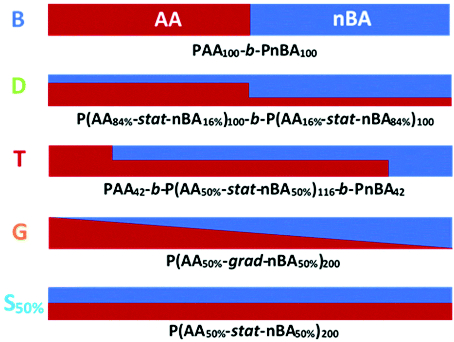 | ||
| Fig. 1 Composition profiles of the five copolymers compared in this study containing the same amount of AA units (50 mol%), but exhibiting different composition profiles: block copolymer (B), asymmetric diblock copolymer (D), asymmetric triblock copolymer (T), linear gradient copolymer (G) and statistical copolymer (S50%). | ||
Experimental part
Polymers
The synthesis of S40%, S50% and S60% has been reported elsewhere.38,39 The synthesis of B, D, T, G,45 S16%, S30%, S70%, S84% and PAA is described in the ESI, section 2.†Materials
All aqueous solutions were prepared using Millipore water (deionized water, resistance > 18 MΩ cm). Sodium chloride (extra pure, Prolabo), hydrochloric acid (HCl 0.1 M, Prolabo) and sodium hydroxide (NaOH 0.1 M, Fisher Sci.) were used as received.Preparation of the solutions
For the titration of polymers containing 50 mol% of AA units in the chain, 30 mL of polymer solution at Cpolymer = 1 g L−1 (corresponding to [AA] = 5 × 10⁻³ mol L−1) and [NaCl] = 0.1 M were prepared as follows. The degree of ionization α of the polymers in their solid form was 0. The polymers were first dissolved in water in the presence of ∼1.1 equivalent of NaOH relative to the total amount of AA units, which was calculated from the chemical structure of the polymer. After stirring for at least one night, the polymers were fully dispersed resulting in transparent solutions. The NaCl concentration was then adjusted using a 4 M NaCl solution. For the statistical copolymers with varying contents of AA, the solutions were prepared in the same way but either at Cpolymer = 1 g L−1 of polymer or at constant [AA] = 5 × 10⁻³ mol L−1.Titration experiments
The polymer solutions were back titrated at room temperature with [HCl] = 0.1 M using an automatic titrator (TIM 856, Radiometer Analytical) controlled by the TitraMaster 85 software. The addition of HCl titrant was done at a constant speed of 0.1 mL min−1. Raw titration data yielded the evolution of the pH of the solution as a function of the volume of titrant (see Fig. S4†). From these data, the total amount of titrable AA units was determined and the evolution of the pH of the solution and of pKaeff of the polymer as a function of α was plotted. Details of the data treatment were reported elsewhere17 and are given in ESI, section 4.†Results and discussion
We first focused on three copolymers with the same overall composition, namely 50 mol% AA and 50 mol% nBA, but with different composition profiles as depicted in Fig. 1. B consists of a pure PAA block connected to a pure PnBA block with the same degree of polymerization. The composition of the gradient copolymer G varies approximately linearly from pure PAA to pure PnBA along the length of the chain. The statistical copolymer S50% contains randomly distributed AA and nBA units. The macromolecular characteristics of the copolymers are displayed in Table 1.| Copolymer | Before acidolysis | After acidolysis | |||
|---|---|---|---|---|---|
M
n![[thin space (1/6-em)]](https://www.rsc.org/images/entities/char_2009.gif) (kg mol−1)
(kg mol−1) |
Đ | tBAb (mol%) | Expected Mnc (kg mol−1) |
AAd (mol%) | |
| a Determined by size exclusion chromatography (SEC) in tetrahydrofuran (THF) before acidolysis for B, and G; determined by SEC in CHCl3 before acidolysis for D and T. SEC was calibrated with poly(methyl methacrylate) (PMMA) standards. For S50%, the analysis was performed on another column calibrated with poly(styrene) (PS) standards.38,39 b Calculated from the molar mass of each block, considering their composition obtained by proton nuclear magnetic resonance (1H NMR). c Number average molar mass (Mn) expected after acidolysis = Mn(before acidolysis) × (ftBA × (MAA/MtBA) + fnBA), where ftBA and fnBA are the mass fractions of tBA and nBA in the polymer before acidolysis which are equal to their molar fractions and were determined by 1H NMR. d The number of moles of AA units nAA titrated in a polymer mass mpol ∼ 30 mg was determined by potentiometric titration. From that, the AA mol% was deduced as: % AA = nAA/(nAA + (mpol − nAA × MAA)/MnBA) where MAA and MnBA correspond to the respective molecular weights of AA or nBA units. For the titration experiments, the typical relative experimental error was lower than 10% as revealed by Fig. S2† which represents two titrations of the same polymers. e The synthesis of S50% was reported previously.38,39 | |||||
| B | 23.2 | 1.12 | 51% | 18.0 | 49% |
| D | 20.9 | 1.10 | 49% | 16.5 | 50% |
| T | 20.1 | 1.07 | 50% | 15.7 | 53% |
| G | 28.9 | 1.35 | 56% | 22.5 | 51% |
| S50%e |
12.5 | 1.10 | 51% | 10.0 | 51% |
All polymers were fully dispersed in aqueous medium in the presence of 10 mol% excess of NaOH to reach α = 1. Thereafter, the polymers were back titrated with HCl at [NaCl] = 0.1 mol L−1. This ensured that the amount of NaCl generated during the titration did not significantly change the ionic strength of the dispersion and, therefore, the titration curve.17 The results were reproducible and not significantly affected by either the molar mass of the polymer or the polymer concentration (see ESI, section 3†) within the investigated conditions. The AA content in the polymers estimated by titration was consistent with the values calculated from the relative mass of the polymer segments and their composition by 1H NMR (see Table 1). This confirmed that all AA units along the polymer chains could be ionized within experimental error as reported elsewhere for similar copolymers.17
The evolution of pH as a function of α was obtained from the raw titration data (see ESI, section 4† and ref. 17) (Fig. 2a). pKaeff = f(α) was calculated from eqn 4 (Fig. 2b). Fig. 2a and b reveal that changes in the composition profile of the copolymers at a constant overall composition (50 mol% of AA units) strongly affected the ionization behavior. For a fixed α, the block copolymer (B, see Fig. 1) exhibited the lowest pKaeff on the full α-range indicating that its AA units were on average more acidic than those of the gradient or the statistical copolymers (G and S50%, see Fig. 1). For both B and G (see Fig. 1), pKaeff strongly increased with α, but for S50% the impact of α on pKaeff was less pronounced.
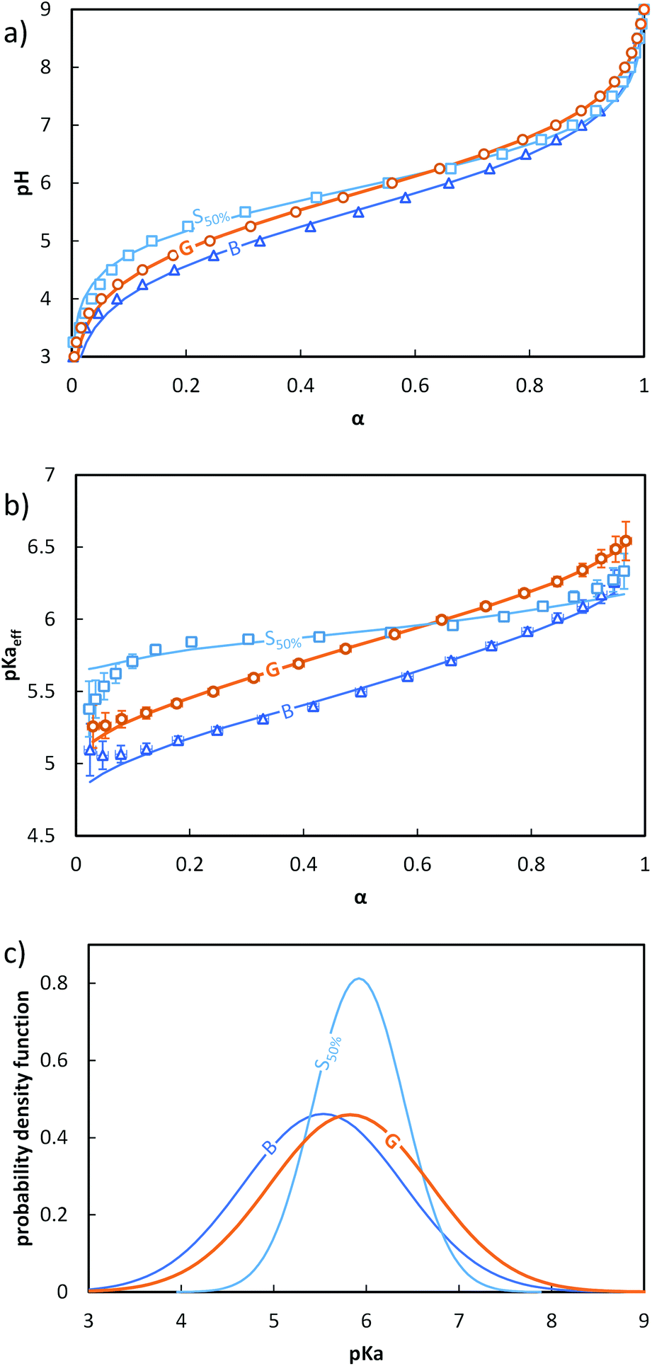 | ||
Fig. 2 Impact of the composition profile on the ionization behavior of copolymers containing 50 mol% of AA units: B (-,  ), G (-, ), G (-,  ) and S50% (-, ) and S50% (-,  ). The titrations were conducted from α = 1 to α = 0 with HCl 0.1 M at a polymer concentration of 1 g L−1 and with 0.1 M NaCl. (a) pH vs. α, (b) pKaeffvs. α, (c) fitted Gaussian distributions of pKa according to eqn (5) (see text). In (a) and (b), the symbols correspond to the experimental data, whereas the lines correspond to the best fit to eqn (5). The fitting parameters are given in Table S4.† ). The titrations were conducted from α = 1 to α = 0 with HCl 0.1 M at a polymer concentration of 1 g L−1 and with 0.1 M NaCl. (a) pH vs. α, (b) pKaeffvs. α, (c) fitted Gaussian distributions of pKa according to eqn (5) (see text). In (a) and (b), the symbols correspond to the experimental data, whereas the lines correspond to the best fit to eqn (5). The fitting parameters are given in Table S4.† | ||
In order to discuss these somewhat qualitative observations in a more quantitative way, the experimental data from Fig. 2a and b were fitted with eqn (5), see section 5a of the ESI† for details.
 | (5) |
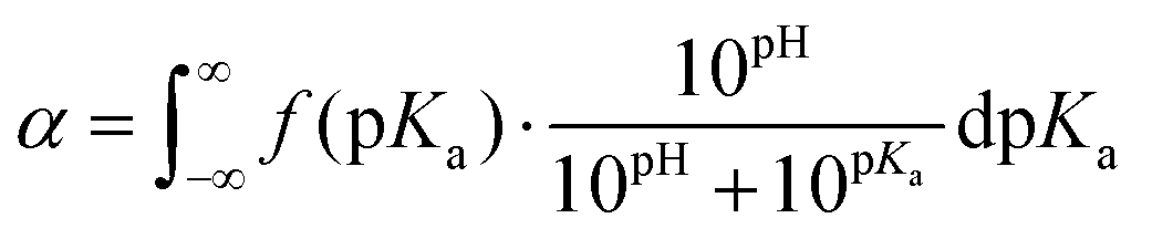
This equation describes the theoretical evolution of α as a function of the pH value for a mixture of ideal monoacids exhibiting a continuous distribution of pKa, f(pKa). An arbitrary Gaussian distribution of pKa was used for f(pKa). This distribution has two parameters: the maximum of the distribution, which corresponds to the average of the distribution, and the standard deviation σ, which corresponds to the width of the distribution (see ESI section 5a† for details). In this “pKa distribution model”, all acids in the distribution have a different pKa, but the pKa values do not vary with α since the acids are considered ideal. Eqn (5) does capture the idea that acidic sites in a weak polyelectrolyte have different environments (even for a homopolymeric polyelectrolyte at a fixed α as underlined in the introduction) and therefore different pKa values. On the contrary, the model assumes no variation of the pKa of the acidic sites with α; which is clearly unrealistic for weak polyelectrolytes. However, from a mathematical point of view, enlarging the distribution of pKa and considering them constant over the whole α range is equivalent to using a narrower distribution of pKa which vary with α.
Therefore, the parameters of the model should be interpreted as follows. First, the absolute values of the pKa over the whole distribution should not be given too much credit because they were obtained by mathematically replacing a variation of pKa with α by a broader distribution of invariant pKa values. Second, the average pKa of the Gaussian distribution physically reflects the mean pKa value of all acidic sites over the whole chain and full α-range and is equal to pKaeff at α = 50%. Third and most importantly, σ reflects the heterogeneity of the acidic character of the AA units. The later originates both from α changes and from variations of the environment of the acidic sites.
Despite having only two parameters, the model described by eqn (5) fits the data well over nearly the entire α-range. The maximum of the distribution followed the order B < G ≈ S50%, while the standard deviation followed the order S50% < G ≈ B (Fig. 2c). The variation of the standard deviation indicated a greater heterogeneity of the acidic sites for G and B than for S50%.
In order to discriminate the effect of the environment of the acidic sites from that of α on the ionizaton and understand the origin of the differences between B, S50% and G, different statistical copolymers of low dispersity were synthesized (see ref. 38, 39 and 45 + ESI, section 2†) and titrated. Each copolymer exhibited a homogeneous composition along the chain but a different AA content ranging from 16 to 84 mol%. A pure PAA homopolymer was also titrated. Fig. 3a and b display their evolution of pH and pKaeff, respectively, as a function of α. From Fig. 3b, it can be deduced that (1) for a given α, the average acidic character decreased with increasing nBA content (pKaeff became larger), (2) for a given nBA content, pKaeff increased with α, and (3) the variation of pKaeff with α was the steepest for PAA, decreased with decreasing AA content (i.e., increasing nBA content) until 40 mol% AA and increased again for even lower AA contents.
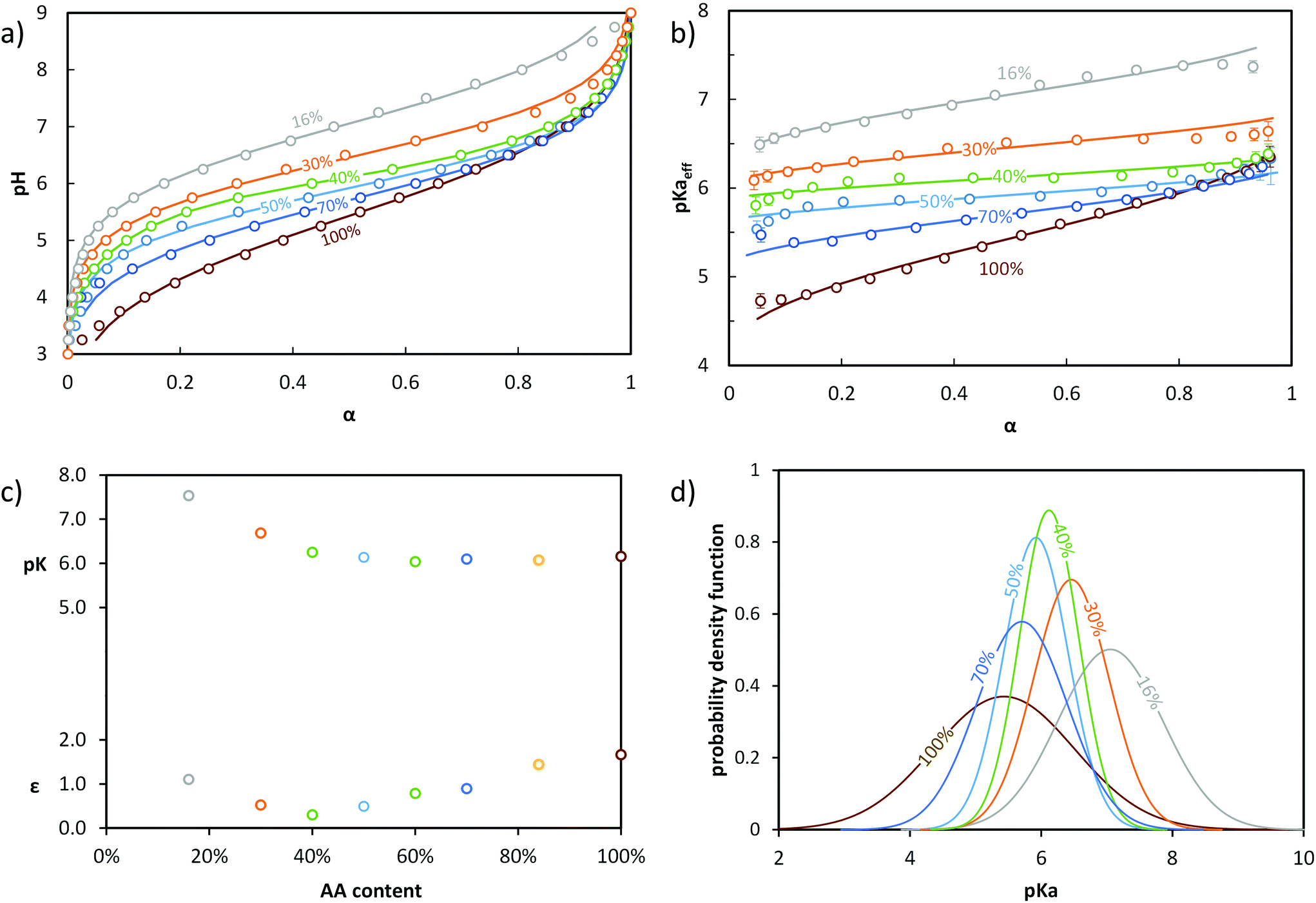 | ||
| Fig. 3 Impact of the AA content (x mol % indicated in the figure) on the ionization behavior of statistical copolymers. The titrations were conducted from α = 1 to α = 0 with HCl 0.1 M at a polymer concentration of 1 g L−1 and with 0.1 M NaCl. (a) pH vs. α, (b) pKaeffvs. α. In (a) and (b), the symbols correspond to the experimental data, whereas the lines correspond to the best fits according to eqn (5) (see text). Data for S84% AA is omitted for clarity, but is shown in Fig. S5.† (c) parameters of the model of Koper and Borkovec11 used to fit the data (details are given in Table S5,† and the corresponding fitted curves are shown in Fig. S6†). (d) Gaussian distributions of pKa obtained from fitting the titration curves to eqn (5) (pdf = probability density function; see Table S4† for fit parameters). | ||
The behavior of these polymers was consistent with previously reported experimental and theoretical work on homogeneously distributed weak polyelectrolytes1 and could be interpreted as follows.
Decreasing the amount of AA (i.e., increasing nBA content) increased the hydrophobic character, resulting in a less polar environment where it was more difficult to create charges. At a fixed α, this effect dominated and caused an increase of pKaeff with decreasing AA content. This trend was clearly reflected by fitting the experimental data with eqn (5) (see Fig. 3). Indeed, the maximum of the distribution increased with decreasing AA content, reflecting a lower overall acidity.
Simultaneously, the steepness of the variation of pKaeff with α first decreased from 100 to 40 mol% AA and then increased again from 40 to 16 mol% AA. Fitting the data with eqn (5) exemplifies and completes these qualitative observations (Fig. 3). σ indeed decreased from 100 to 40 mol% of AA and increased again from 40 to 16 mol% AA, reflecting first a decrease of the heterogeneity of the acidic sites down to 40 mol% AA and then an increase. The heterogeneity of the acidic sites quantified by σ could be attributed to a large extent to the variation with α of the interactions between charges. Decreasing the amount of AA units resulted in an increased distance between them, causing interactions to play a lesser role. This effect dominated from 100 to 40 mol% AA, resulting in a shallower increase of pKaeff with α as the AA content decreased. Additionally, the presence of hydrophobic nBA units in the copolymers resulted in their collapse into small spherical aggregates of several nanometers at lower α39,45 as previously observed by light scattering. This forced the AA units closer to one another and affected the interactions. This probably enhanced both the variation of pKaeff with α (because the extent of aggregation depends on α)39 and the heterogeneity of the acidic sites at a given α (because the environment of the AA units is not the same within the aggregates or close to their surface), both phenomena increasing σ. The impact of aggregation apparently dominated between 40 and 16 mol% AA, resulting in an increase of σ with decreasing AA content.
We also note that the titration curves of the statistical copolymers could also be fitted to a model described by Koper and Borkovec11 using two parameters: pK, which represents the acidic character of the AA units at α = 1 and ε, which represents the extent of coupling between the neighboring AA units (see section 5b of the ESI† and Fig. 3c). The variations of pK and ε qualitatively follow those of the maximum of the Gaussian distribution and of σ, respectively, and can be qualitatively interpreted in the same way.
To summarize, the pKa of the acidic units in a copolymer depends on (1) the AA content, (2) α, the effect being attenuated by spacing the monomer units from each other and (3) to a lesser extent, the collapse of the chain due to hydrophobic interactions. In a statistical copolymer, the AA content hardly varies along the chain. Therefore, the heterogeneity of the acidic sites reflected by σ is mainly caused by the effect of α and, to some extent, by the collapse of the chain at low AA contents. Changing the proportion of AA units however causes huge variations of pKaeff (at constant α) between distinct statistical copolymers with different AA contents.
In a gradient copolymer, the AA content varies along the chain. Based on the results on the statistical copolymers, we concluded that the broad distribution of apparent pKa observed for G (Fig. 2c) reflects both the decrease in overall acidic character with increasing α due to repulsive electrostatic interactions, and the spatial heterogeneity of the individual acidic sites caused by the heterogeneous composition profile along the polymer chain, as depicted in Fig. 4. More precisely, we speculated that the AA units at one end of a gradient copolymer would behave like an AA-rich statistical copolymer, while AA units further along the chain would behave like statistical copolymers with decreasing AA content. In other words, the gradient copolymer would behave like a combination of statistical copolymers of different compositions.
 | ||
| Fig. 4 Idealized distribution of charges for S50%, B, G and T at pH = 5 determined based on our results (see Fig. 2a, 3a and 5 for the average values of α for each copolymer and text for the rationale behind this scheme). For S50%, α ∼ 14% and the charges are roughly evenly distributed. For B, the PAA block is ionized at α ∼ 33% and the charges are roughly evenly distributed within this block, except close to the PnBA block where ionization is more difficult because of the self-assembly into micelles. For T, α ∼ 26% on average, but the PAA block is much more ionized (∼38%) than the statistical P(AA-co-nBA) block (∼14%), whereas the PnBA block contains no charges. Finally, G has roughly the same titration curve as T, which strongly suggests a heterogeneous distribution of charges along the chain due to the heterogeneous composition profile of the comonomers. | ||
To test this hypothesis, we tried to mimic the titration curve of the gradient copolymer as a combination of a limited number of blocks with compositions varying stepwise rather than continuously as in the gradient copolymer. This was first tested by synthesizing a series of di- and tri-block copolymers with composition profiles that approximated ever more closely that of the gradient copolymer (see ESI section 1†). These composition profiles consisted of: a block copolymer (B) of two blocks of equal length, containing 0 and 100 mol% of AA respectively; an asymmetric diblock copolymer (D) of two blocks of equal length containing 16 and 84 mol% of AA respectively; and an asymmetric triblock copolymer (T) of two blocks of equal length, containing 0 and 100 mol% of AA respectively, separated by a central statistical block containing 50 mol% of AA that accounted for 58 mol% of the total length of the polymer. The chemical structures of the corresponding block copolymers are represented in Fig. 1, their macromolecular characteristics are summarized in Table 1. These polymers were designed so that they contained the same total overall amount of AA units as G. Moreover, D and T exhibited the same average position of the AA units in the chain (see ESI section 1†). Their titration curves are displayed in Fig. 5. Fig. 5a and b revealed that B was a very poor experimental mimic of the gradient copolymer. This result was already discussed above (Fig. 2) and is not surprising because of the abrupt variation of composition along the chain for B as compared to G. D, which resembled B but with a weaker variation of composition between each block behaved more similarly to the gradient copolymer, but still did not capture faithfully its ionization behavior. Finally, T, which contains a central block of statistical AA/nBA copolymer resulting in a smoother evolution of the AA content along the polymer chain, behaved very similarly to the gradient copolymer. These results support our initial hypothesis that the behavior of a complex gradient copolymer exhibiting a continuous variation of composition along the chain can be mimicked by asymmetrical block copolymers exhibiting a small number of step changes in their composition profile.
 | ||
Fig. 5 Comparison of the ionization behavior of model copolymers mimicking the behavior of the gradient. The titrations were conducted from α = 1 to α = 0 with HCl 0.1 M at a polymer concentration of 1 g L−1 and with 0.1 M NaCl. (a) pH vs. α for B ( ), D ( ), D ( ), T ( ), T ( ) and G ( ) and G ( ). The pH-axis was enlarged to highlight the small differences between the polymers. (b) pKaeffvs. α for B, D, T, G. (c) Gaussian distributions of pKaeff for B, D, G, T. Lines in (a) and (b) correspond to fits to eqn (5). The fitting parameters are given in Table S4.† ). The pH-axis was enlarged to highlight the small differences between the polymers. (b) pKaeffvs. α for B, D, T, G. (c) Gaussian distributions of pKaeff for B, D, G, T. Lines in (a) and (b) correspond to fits to eqn (5). The fitting parameters are given in Table S4.† | ||
To go one step further, we attempted to mimic the titration curves of each of these model copolymers (B, D, T) by mathematically combining the titration curves of their component statistical blocks. This was done by taking into account the molar fraction of AA units contained in each of these blocks and assuming that the covalent bond between the different blocks did not affect each block's titration behavior (see ESI, section 6†). If this assumption holds, B should behave as a pure PAA homopolymer. This was, however, not the case as shown in Fig. 6a which revealed a strong discrepancy between the experimental titration curve of B and the corresponding mathematical model at α ≤ 50%. This discrepancy can probably be attributed to the fact that B self-assembled into spherical micelles in aqueous medium45 and, therefore, had a star-like architecture.
 | ||
Fig. 6 Mathematical modelling of the evolution of pKaeffvs. α for (a) B ( ), modelled as a pure PAA block ( ), modelled as a pure PAA block ( ), (b) D ( ), (b) D ( ), modelled as 16 mol% S16% + 84 mol% S84% ( ), modelled as 16 mol% S16% + 84 mol% S84% ( ) and (c) T ( ) and (c) T ( ), modelled as 42 mol% PAA + 58 mol% S50% ( ), modelled as 42 mol% PAA + 58 mol% S50% ( ). G ( ). G ( ) is also represented for comparison on each curve (the line connecting the points is only to guide the eye). The experimental data and conditions used in this figure are the same as in Fig. 5. ) is also represented for comparison on each curve (the line connecting the points is only to guide the eye). The experimental data and conditions used in this figure are the same as in Fig. 5. | ||
As explained in the introduction, such an architecture decreases the acidic character of the units closest from the star center, whereas those at the end of the arms behave like linear polymers.11,13–16 Overall, this increases pKaeff at a given α46,47 compared to a linear PAA as observed here at low α where the effect is the strongest. D is mathematically modelled in Fig. 6b as a combination of S16% and S84%. The discrepancy between the mathematical model and the experimental data was still significant, but much less pronounced than for B at low α. We attributed the better agreement between the mathematical model and the experimental data to the fact that both S16% and D self-assembled in aqueous medium, so that the impact of self-assembly was not as strong as between PAA homopolymer (not self-assembled) and B (strongly self-assembled).
Finally, for T, the agreement between the mathematical model and the experimental curve was significantly improved (Fig. 6c). Moreover, both curves for T were very similar to that of the gradient copolymer, supporting the idealized picture of the distribution of ionized acidic groups shown in Fig. 4.
We tested numerous combinations of AA homopolymer and statistical copolymers, and found that the gradient curve was best fit by triblock copolymers with a composition profile consisting of initial and final blocks of 100 mol% AA and 16 mol% AA and a central block of intermediate composition (between 40 mol% and 70 mol% AA). Good fits were obtained when the lengths of each block were selected such that the overall composition in AA was 50 mol%, and the first moment of the position distribution of the AA units was identical to that of the gradient copolymer (see ESI section 6† for full details).
This result is interesting from an application point of view because it indicates that a good approximation of the titration behavior of a 20 kg mol−1 (DPn ∼ 200) gradient copolymer can be obtained using only three segments of statistical copolymers (see Fig. 5). It further suggests that the titration curves of weak polyelectrolytes could be tuned in a predictable way by modifying the composition profile of copolymers with no more than three statistical segments. Moreover, these results could also be used to adapt the existing theories and models currently valid for weak polyelectrolytes exhibiting a homogeneous composition profile to more complex weak polyelectrolytes such as gradient copolymers or block copolymers with step-wise variation of their composition profile.
Conclusions
In this paper, we investigated the ionization behavior of weak polyacids consisting of AA and nBA units. It was shown that for a constant composition of AA units within the copolymer chain (50 mol%), the titration curve of the polymers could be altered by varying the composition profile along the chain. A gradient copolymer exhibiting a continuous (linear) change of the composition along the chain exhibited a strong heterogeneity of acidic sites along the chains. This could be rationalized by studying statistical copolymers with varying AA contents. The broad distribution of pKa observed for the gradient copolymers was caused not only by the decrease of their acidic character with increasing α due to repulsive electrostatic interactions, but also by the spatial heterogeneity of the individual acidic sites along the polymer chain.Moreover, we showed that the gradient copolymer could be mimicked both synthetically and mathematically by triblock copolymers exhibiting a step-wise rather than a continuous composition profile along the chain. Our findings strongly simplify the description of gradient copolymers. From a fundamental point of view, this would allow existing theories and models to be adapted to gradient copolymers. From an application point of view, these results suggest that the titration curves of weak polyelectrolytes could be tuned in a predictable way by modifying the composition profile of copolymers with no more than three statistical segments.
Conflicts of interest
There are no conflicts to declare.Acknowledgements
U. S. S. and C. G. S. thank the Center for Excellence “PolyTarget” (SFB 1278, projects A01, B02, and Z01 316213987) of the Deutsche Forschungsgemeinschaft (DFG, Germany) for financial support. J. Z. would like to thank National Natural Science Foundation of China (21901208) and Natural Science Basic Research Plan in Shaanxi Province of China (2020JQ-138) for financial support. This research was financially supported in part by the ASYMCOPO Project, an international collaborative research project of the DFG and the Agence Nationale de la Recherche (ANR, France); DFG project: GU 1685/1-1 and ANR project ANR-15-CE08-0039. BFM acknowledges financial support from CONACyT (Consejo Nacional de Ciencia y Tecnología, México). Taco Nicolai is thanked for helpful discussions.Notes and references
- J. Landsgesell, L. Nova, O. Rud, F. Uhlık, D. Sean, P. Hebbeker, C. Holm and P. Kosovan, Soft Matter, 2019, 15, 1155–1185 RSC
.
- X. Jia and K. L. Kiick, Macromol. Biosci., 2009, 9, 140–156 CrossRef CAS
- C. Chassenieux and C. Tsitsilianis, Soft Matter, 2016, 12, 1344–1359 RSC
- J. Jagur-Grodzinski, Polym. Adv. Technol., 2010, 21, 27–47 CrossRef CAS
- J. Höpfner, T. Richter, P. Kosovan, C. Holm and M. Wilhelm, Prog. Colloid Polym. Sci., 2013, 140, 247–263 Search PubMed
- T. Richter, J. Landsgesell, P. Kosovan and C. Holm, Desalination, 2017, 414, 28–34 CrossRef CAS
- N. A. Peppas, P. Bures, W. Leobandung and H. Ichikawa, Eur. J. Pharm. Biopharm., 2000, 50, 27–46 CrossRef CAS
-
M. Nagasawa, in Advances in Chemical Physics - Physical Chemistry of Polyelectrolyte solutions, ed. S. A. Rice and A. R. Dinner, Wiley, 2015, vol. 158, pp. 67–114 Search PubMed
- C. Holm, J. F. Joanny, K. Kremer, R. R. Netz, P. Reineker, C. Seidel, T. A. Vilgis and R. G. Winkler, Adv. Polym. Sci., 2004, 166, 67–111 CrossRef CAS
- I. Borukhov, D. Andelman, R. Borrega, M. Cloitre, L. Leibler and H. Orland, J. Phys. Chem. B, 2000, 104, 11027–11034 CrossRef CAS
- G. J. M. Koper and M. Borkovec, Polymer, 2010, 51, 5649–5662 CrossRef CAS
- M. Castelnovo, P. Sens and J.-F. Joanny, Eur. Phys. J. E: Soft Matter Biol. Phys., 2000, 1, 115–125 CrossRef CAS
- C. Qu, Y. Shi, B. Jing, H. Gao and Y. Zhu, ACS Macro Lett., 2016, 5, 402–406 CrossRef CAS
- P. Matejicek, K. Podhajecka, J. Humpolickova, F. Uhlik, K. Jelinek, Z. Limpouchova and K. Prochazka, Macromolecules, 2004, 37, 10141–10154 CrossRef CAS
- F. Uhlík, P. Kosovan, Z. Limpouchova, K. Prochazka, O. V. Borisov and F. A. M. Leermakers, Macromolecules, 2014, 47, 4004–4016 CrossRef
- V. S. Rathee, H. Sidky, B. J. Sikora and J. K. Whitmer, Polymers, 2019, 11, 183 CrossRef
- O. Colombani, E. Lejeune, C. Charbonneau, C. Chassenieux and T. Nicolai, J. Phys. Chem. B, 2012, 116, 7560–7565 CrossRef CAS
- M. Fowler, B. Siddique and J. Duhamel, Langmuir, 2013, 29, 4451–4459 CrossRef CAS
- Y. Zhao, Y.-W. Luo, B.-G. Li and S. Zhu, Langmuir, 2011, 27, 11306–11315 CrossRef CAS
- W. van Riemsdijk, L. Koopal, D. G. Kinniburgh, M. F. Benedetti and L. Weng, Environ. Sci. Technol., 2006, 40, 7473–7480 CrossRef CAS
- A. C. Montenegro, S. Orsetti and F. V. Molina, Environ. Chem., 2014, 11, 318–332 CrossRef CAS
- A. Piccolo, Soil Sci., 2001, 166, 810–832 CrossRef CAS
- H. K. Murnen, A. R. Khokhlov, P. G. Khalatur, R. A. Segalman and R. N. Zuckermann, Macromolecules, 2012, 45, 5229–5236 CrossRef CAS
- P. G. Khalatur and A. R. Khokhlov, Adv. Polym. Sci., 2006, 195, 1–100 CrossRef CAS
- A. R. Khokhlov and P. G. Khalatur, Curr. Opin. Colloid Interface Sci., 2005, 10, 22–29 CrossRef CAS
- D. D. Bendejacq, V. Ponsinet and M. Joanicot, Langmuir, 2005, 21, 1712–1718 CrossRef CAS
- D. B. Wright, J. P. Patterson, A. Pitto-Barry, P. Cotanda, C. Chassenieux, O. Colombani and R. K. O'Reilly, Polym. Chem., 2015, 6, 2761–2768 RSC
- O. Borisova, L. Billon, M. Zaremski, B. Grassl, Z. Bakaeva, A. Lapp, P. Stepanek and O. Borisov, Soft Matter, 2012, 8, 7649–7659 RSC
- O. Borisova, L. Billon, M. Zaremski, B. Grassl, Z. Bakaeva, A. Lapp, P. Stepanek and O. Borisov, Soft Matter, 2011, 7, 10824–10833 RSC
- G. Laruelle, J. François and L. Billon, Macromol. Rapid Commun., 2004, 25, 1839–1844 CrossRef CAS
- M. Rabyk, A. L. Destephen, A. Lapp, S. King, L. Noirez, L. Billon, M. Hruby, O. Borisov, P. Stepanek and E. Deniau, Macromolecules, 2018, 51, 5219–5233 CrossRef CAS
- C. Charbonneau, C. Chassenieux, O. Colombani and T. Nicolai, Macromolecules, 2011, 44, 4487–4495 CrossRef CAS
- C. Charbonneau, C. Chassenieux, O. Colombani and T. Nicolai, Macromolecules, 2012, 45, 1025–1030 CrossRef CAS
- C. Charbonneau, M. D. S. Lima, C. Chassenieux, O. Colombani and T. Nicolai, Phys. Chem. Chem. Phys., 2013, 15, 3955–3964 RSC
- C. Charbonneau, T. Nicolai, C. Chassenieux, O. Colombani and M. D. S. Lima, React. Funct. Polym., 2013, 73, 965–968 CrossRef CAS
- F. Dutertre, O. Boyron, B. Charleux, C. Chassenieux and O. Colombani, Macromol. Rapid Commun., 2012, 33, 753–759 CrossRef CAS
- E. Lejeune, C. Chassenieux and O. Colombani, Prog. Colloid Polym. Sci., 2011, 138, 7–16 CAS
- E. Lejeune, M. Drechsler, J. Jestin, A. H. E. Müller, C. Chassenieux and O. Colombani, Macromolecules, 2010, 43, 2667–2671 CrossRef CAS
- L. Lauber, C. Chassenieux, T. Nicolai and O. Colombani, Macromolecules, 2015, 48, 7613–7619 CrossRef CAS
- L. Lauber, O. Colombani, T. Nicolai and C. Chassenieux, Macromolecules, 2016, 49, 7469–7477 CrossRef CAS
- L. Lauber, J. Depoorter, T. Nicolai, C. Chassenieux and O. Colombani, Macromolecules, 2017, 50, 8178–8184 CrossRef CAS
- L. Lauber, J. Santarelli, O. Boyron, C. Chassenieux, O. Colombani and T. Nicolai, Macromolecules, 2017, 50, 416–423 CrossRef CAS
- A. Shedge, O. Colombani, T. Nicolai and C. Chassenieux, Macromolecules, 2014, 47, 2439–2444 CrossRef CAS
- J. Zhang, B. Farias-Mancilla, M. Destarac, U. S. Schubert, D. J. Keddie, C. Guerrero-Sanchez and S. Harrisson, Macromol. Rapid Commun., 2018, 39, 1800357 CrossRef
- J. Zhang, B. Farias-Mancilla, I. Kulai, S. Hoeppener, B. Lonetti, S. Prévost, J. Ulbrich, M. Destarac, O. Colombani, U. S. Schubert, C. Guerrero-Sanchez and S. Harrisson, Angew. Chem., Int. Ed., 2020 DOI:10.1002/anie.202010501
- F. A. Plamper, H. Becker, M. Lanzendörfer, M. Patel, A. Wittemann, M. Ballauff and A. H. E. Müller, Macromol. Chem. Phys., 2005, 206, 1813–1825 CrossRef CAS
-
Y. Xu, F. Plamper, M. Ballauff and A. H. E. Müller, in Complex Macromolecular Systems II. Advances in Polymer Science, ed. A. H. E. Müller and H. W. Schmidt, SPRINGER-VERLAG BERLIN, Berlin, 2010, vol. 228, pp. 1–38 Search PubMed
Footnote |
| † Electronic supplementary information (ESI) available: 1. Explanation of the profile of the G, B, D, T copolymers; 2. polymer synthesis; 3. control titration experiments; 4. typical raw titration curve; 5. fits; 6. mathematical combination of the titration data. See DOI: 10.1039/d0py01059f |
| This journal is © The Royal Society of Chemistry 2020 |