 Open Access Article
Interpretable machine learning as a tool for scientific discovery in chemistry
Richard
Dybowski
 *
*
St John's College, University of Cambridge, Cambridge CB2 1TP, UK. E-mail: rd460@cam.ac.uk
First published on 9th November 2020
Abstract
There has been an upsurge of interest in applying machine-learning (ML) techniques to chemistry, and a number of these applications have achieved impressive predictive accuracies; however, they have done so without providing any insight into what has been learnt from the training data. The interpretation of ML systems (i.e., a statement of what an ML system has learnt from data) is still in its infancy, but interpretation can lead to scientific discovery, and examples of this are given in the areas of drug discovery and quantum chemistry. It is proposed that a research programme be designed that systematically compares the various model-agnostic and model-specific approaches to interpretable ML within a range of chemical scenarios.
1 AI and ML
Artificial intelligence (AI) is a large and complex subfield of computer science concerned with the development of algorithms that mimic (to some degree) human cognitive functions such as learning, image recognition and natural language processing.1 It is believed that induction (generalising from finite examples) is an innate cognitive attribute,2 and induction is the core interest of machine learning (ML),3 which has become a prominent part of AI.Numerous techniques have been developed under the heading of ML including neural networks, support vector machines and random forests,4 but, in line with the concept of ‘statistical learning’,5 we will also regard all forms of statistical regression as being under the ML umbrella.
1.1 Deep learning
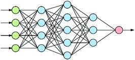
At the heart of neural-based computation is the concept of an artificial neural network.6 The term “deep neural networks” (DNNs) refers to neural networks that have several internal layers of neurons (Fig. 1), and their strength lies in their ability to make multiple non-linear transformations through these layers of neurons.7 In this process, increasingly complex and abstract features can be constructed by the addition of more layers and/or increasing the number of neurons per layer. Each layer can be thought of as performing an abstraction of the information held within the preceding layer, so that a sequence of layers provides a hierarchy of increasing abstraction. This can obviate the need for manual selection of input features.1.2 Convolutional neural networks
Convolutional neural networks (CNNs) are a subclass of DNNs. CNNs8 are inspired by the Hubel–Wiesel model of the visual primary cortex9 in which complex images are built up from simple features. The standard architecture of a CNN consists of alternating convolutional and pooling layers. A convolutional layer preserves the relationship between values in a matrix by multiplying a submatrix of the layer with a matrix filter to produce a ‘feature map’. As a result, the network learns filters that activate when it detects some specific type of feature at some spatial position in the input.A pooling layer abstracts the values of a feature map. This successive use of convolutional and pooling layers produces a hierarchy of abstracted features from an image that are invariant to translation, hence the successful use of CNNs for the recognition of images such as faces.
2 ML for chemistry
ML techniques, such as deep neural networks, have become an indispensable tool for a wide range of applications such as image classification, speech recognition, and natural language processing. These techniques have achieved extremely high predictive accuracy, in many cases, on par with human performance.There are many examples of where ML has been applied within chemistry,10 including the design of crystalline structures,11 planning retrosynthesis routes,12 and reaction optimisation.13 Here, we will briefly look at two; namely, drug discovery and quantum chemistry.
2.1 Drug discovery
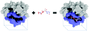
The purpose of drug discovery is to find a compound that will dock with a biomolecule believed to be associated with a disease of interest (Fig. 2).Once a target biomolecule (usually a protein) that is associated with a disease enters a pharmaceutical company's pipeline, it can take about 12 years to develop a marketable drug, but the failure rate during this process is high and costly. Each new drug that does reach the market represents research and development costs of close to one billion US dollars; therefore, early drug validation is vital, and this has led to the rise of computational (in silico) techniques.14 Consequently, the traditional techniques for drug discovery and target validation15,16 have been augmented with the use of machine learning to reduce the number of candidates by predicting whether a chemical substance will have activity at a given target.17 An example is the use of an ANN to aid the design of anti-bladder cancer agents.18
The standard approach to developing a neural network to predict whether a compound S will be active with respect to a target protein P is to train the network using a collection {S1,…,Sn} of compounds with known activity toward P, but how can a ligand–protein activity predictor be trained if there are no known ligands for target protein P? AtomNet19 is a CNN designed to predict ligand–protein activities when no ligand activity for a target protein is available. This is done by training the CNN using known activities across a range of ligand–protein complexes. The thesis of AtomNet is as follows: (i) a complex ligand–protein interaction can be viewed as a combination of smaller and smaller pieces of chemical information; (ii) a CNN can model hierarchical combinations of simpler items of information; (iii) therefore, a CNN can model complex ligand–protein interactions.
Ligand–protein associations were encoded for AtomNet using ligand–protein interaction Fingerprints. The network significantly outperformed a variant of AutoDock Vina;20 for example, AtomNet achieved an AUC (Area Under ROC Curve) greater than 0.9 for 57.8% of the targets in the DUDE dataset (Directory of Useful Decoys [false positives]).21
It is important when using ML for drug discovery that the ligand–protein data used to test the ML system is not biased.22
2.2 Quantum chemistry
The eigenvalue of the electronic Schrödinger equation HΨ = EΨ gives total energy E, were H is the Hamiltonian operator and Ψ the wave function, but solving the equation analytically is limited to a few very simple cases. Therefore, for larger molecules, numerical approximation has been proposed, but with these methods, increasing accuracy is achieved at the cost of increasing run time (Table 1). Consequently, turning to ML was done to see if this enables E to be estimated for larger molecules in radically shorter times without loss of accuracy (Fig. 3).| Method | Runtime |
|---|---|
| Configuration interaction (up to quadruple excitations) | O(N10) |
| Coupled cluster (CCSD(T)) | O(N7) |
| Configuration interaction (single and double excitations) | O(N6) |
| Møller–Plesset second-order perturbation theory | O(N5) |
| Hartree–Fock | O(N4) |
| Density functional theory (Kohn–Sham) | O(N3–4) |
| Tight binding | O(N3) |
| Molecular mechanics | O(N2) |
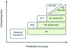 | ||
| Fig. 3 Schematic representation of quantum chemical and ML approximations with respect to computational cost and accuracy, which generalises the literature.24 DFT = density functional theory; SQC = semi-quantitative quantum chemistry. | ||
The set of nuclear charges {Zi} and atomic Cartesian coordinates {Ri} uniquely determine the Hamiltonian H of any chemical compound,
An example of the use of ML for quantum chemistry is the mapping of {Z,R} to E by encoding the information in {Z,R} using a Coulomb matrix M:25
The data set {Mk,Erefk} consisted of 7165 organic compounds, encoded as Coulomb matrices M, along with their energies Eref calculated using the PBE0 density function model. Cross-validation gave a mean absolute prediction error of 9.9 kcal mol−1.
3 Scientific discovery
The examples shown in the previous section focused on the use of ML for prediction, but what about scientific insight? Neural networks are so-called ‘black-box’ systems, meaning that the mapping of a vector of input values to a neural network's output is too computationally complex for a human to comprehend; therefore, how can we, for example, discover what chemistry the AtomNet CNN has learnt from the vast amount of ligand–protein-interaction data used to train it for in silico drug screening?The idea of using AI for scientific discovery is not new,26 and there has recently been interest in using ML to provide scientific insights as well as making accurate predictions.27
3.1 Interpretable ML
Currently, an important requirement of AI systems is not only the accuracy of the conclusions reached by the systems but also transparency as to how the conclusions were reached. Algorithms, particularly ML algorithms, are increasingly important to peoples' lives, but they have caused a range of concerns revolving mainly around unfairness, discrimination and opacity. This has led to a “right to an explanation” under the EU General Data Protection Regulation.Interpretability is an ill-defined concept,28 but it will suffice for us to use the definition that interpretable ML is the use of ML models for the extraction of relevant knowledge about domain relationships contained in data.29 Consequently, interpretability refers to the extent to which a human expert can comprehend what an ML system has learnt from data; for example, “What is this ML system telling us?” From an interpretation we have insight, and from insight we can hopefully make a scientific discovery.
There are several categories of interpretability in the context of ML. In the following list, f(x) will be written as  , where
  is the set of ML parameters estimated from training data.
(a) Observe the input–output behaviour of  ; for example, by observing how
  varies as x is varied.
(b) Inspect the values of parameters  within the internal structure of
  . Here,
  is either intrinsically interpretable or is interpretable by design. This allows mapping
  to be understood by a series of steps going from input x to output
  that are comprehensible to a domain expert. This can be regarded as an ‘explanation’ of how
  was derived from x.
(c) Determine the prototypical value x of for a given specific value f* of  . Conceptually, this can be regarded as the x that maximises conditional probability p(x|f*). x need not have been previously encountered in a training set. An example of this approach is activation maximization.30
A simple example of an intrinsically interpretable ML system is a linear regression model
The potential of using interpretable ML for chemistry is starting to grow. For example, Bayesian neural networks have been optimised to predict the dissociation time of the unmethylated and tetramethylated 1,2-dioxetane molecules from only the initial nuclear geometries and velocities.32 Conceptual information was extracted from the large amount of data produced by simulations.
We now look at two other examples of interpretable ML: one from drug discovery; the other from quantum chemistry.
3.2 Drug discovery and interpretability
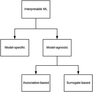
There are generally two approaches to providing interpretable ML: the model-agnostic and model-specific approaches (Fig. 4). Model-agnostic methods are, in principle, applicable to any black-box ML system f(x), whereas the model-specific approach uses a domain-specific ML system, the structure of which is (at least partly) meaningful within the domain of interest.There are two types of model-agnostic techniques. One method is the association-based technique in which associations are determined between inputs to system f(x) and outputs from the system. One example of this are partial dependency plots,5 which create sets of ordered pairs {(x(i)s,f(x(i)s)} where feature subset xs ⊂ x. Another way to examine how f(x) changes as xj (xj ∈ x) changes is to use the ‘gradient input’  , where
  is a particular value of xi. However, an extension of this is to integrate the gradient along a path for xi from observed value
  to a baseline value
  . This is called an ‘integrated gradient’:
Integrated gradients33 determined the chemical substructures (toxicophores) that are important for differentiating toxic and non-toxic compounds. The relevant substructures identified in 12 compounds randomly sampled from the Tox21 Challenge data set are shown in Fig. 5. The DNN consisted of four hidden layers, each with 2048 nodes. The molecular structures were encoded using ECFPs, the training and test sets had 12![[thin space (1/6-em)]](https://www.rsc.org/images/entities/char_2009.gif) 060 and 647 examples, respectively, and the resulting AUC was 0.78.
060 and 647 examples, respectively, and the resulting AUC was 0.78.
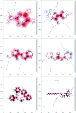 | ||
| Fig. 5 Six randomly drawn Tox21 samples. Dark red indicates that these atoms are responsible for a positive classification, whereas dark blue atoms attribute to a negative classification.33 | ||
An alternative to the detection of features relevant to a classification performed by a DNN is to start at an output node and work back to the input nodes. This is done with Layer-Wise Relevance Propagation (LRP),34 which uses the network weights and the neural activations of a DNN to propagate the output (at layer M) back through the network up until the input layer (layer 1). The backward pass is a conservative relevance redistribution procedure where those neurons in layer l (1 ≤ l < M) that contribute the most to layer l + 1 receive the most ‘relevance’ from it. LRP has, so far, only been used to detect relevant features in pixel-based images and has not been used for the interpretation of chemistry-oriented ML systems. For example, rather than use fingerprints, such as ECPF, for molecular structure input, 2D molecular drawings have been used as inputs to a CNN (and achieved a predictive accuracy of AUC 0.766)35 but LRP was not used for interpretation.
Graph convolutional neural networks (GCNNs) are a variant of CNNs that enable 3D graphs to be used as inputs. Consequently, if the nuclei and bonds of a compound are regarded as the vertices and edges of a 3D graph then 3D molecular structures can be considered as inputs to GCNNs. One approach is to initially slide convolutional filters over atom pairs to obtain atom-pair representations;33 pooling is then used to produce simple substructure representations. These representations were then fed into the next convolutional layer. The predictive accuracy of the resulting GCNN was an AUC of 0.714. Interpretation was done by omitting the pooling steps and feeding the substructures directly into the fully connected network.
The other type of model-agnostic approach is the use of surrogates (Fig. 6); namely, using a function ![[f with combining tilde]](https://www.rsc.org/images/entities/i_char_0066_0303.gif) (x) that is an approximation of black box f(x) but which is intrinsically interpretable. Examples of parsimonious intrinsically interpretable models include linear regression, logistic regression and decision trees. Such models can be either global or local. Given a set of vectors {x(1),…,x(n)}nd that we wish to apply to f(x), the global approach is to apply each of these vectors to the same surrogate model
(x) that is an approximation of black box f(x) but which is intrinsically interpretable. Examples of parsimonious intrinsically interpretable models include linear regression, logistic regression and decision trees. Such models can be either global or local. Given a set of vectors {x(1),…,x(n)}nd that we wish to apply to f(x), the global approach is to apply each of these vectors to the same surrogate model ![[f with combining tilde]](https://www.rsc.org/images/entities/i_char_0066_0303.gif) (x). In contrast, the local approach uses a different surrogate model
(x). In contrast, the local approach uses a different surrogate model ![[f with combining tilde]](https://www.rsc.org/images/entities/i_char_0066_0303.gif) i(x(i)) for vector x(i). An example is the LIME technique,36 which trains
i(x(i)) for vector x(i). An example is the LIME technique,36 which trains ![[f with combining tilde]](https://www.rsc.org/images/entities/i_char_0066_0303.gif) i(x(i)) on data in the ‘neighbourhood’ of x(i), thereby providing interpretability specifically for the input–output pair (x(i),
i(x(i)) on data in the ‘neighbourhood’ of x(i), thereby providing interpretability specifically for the input–output pair (x(i), ![[f with combining tilde]](https://www.rsc.org/images/entities/i_char_0066_0303.gif) i(x(i))).
i(x(i))).
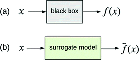 | ||
Fig. 6 (a) Black box trained from data {x,y}. (b) Surrogate model of the black box trained from the same data. ![[f with combining tilde]](https://www.rsc.org/images/entities/i_char_0066_0303.gif) (x) approximates f(x). (x) approximates f(x). | ||
3.3 Quantum chemistry and interpretability
The above perspectives to interpreting a neural network focus on discovering associations between values at the input and output nodes: values at the hidden nodes are ignored. In contrast, another way of attempting to produce interpretable neural networks is to use internal nodes that are meaningful with respect to a domain of interest. This idea is not new and is at the heart of neuro-fuzzy systems37 in which the interpretability of a neural network is provided by chains of inference via fuzzy logic.38Rather than resorting to fuzzy logic, neural networks such as SchNet (described below) are constructed by combining science-based subsystems in a plausible manner. This is an example of the model-specific approach to interpretable ML (Fig. 4).
A strategy for molecular energy E prediction39 is to represent each atom i by a vector ci in B-dimensional space, and a deep tensor neural network (DTNN) called SchNet, shown in Fig. 7, repeatedly refines ci by pair-wise interaction between atoms i and j from an initial vector c(0)i for atom i to final vector c(T)i:
 | (1) |
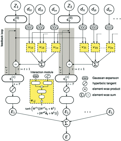 | ||
| Fig. 7 The architecture of SchNet.39 The iteration loop implements eqn (1), and the interaction module (a neural network) implements eqn (2). | ||
Term vij is obtained from atom vector cj and distance dij using a feedforward neural network with a tanh activation function:
| vij = tanh[Wfc(Wcfcj + bf1) ○ (Wdfdij + bf2)] | (2) |
After T iterations, an energy contribution Ei for atom i is predicted for the final vector c(T)i, and the total energy E is the sum of the predicted contributions Ei.
The DTNN, trained using stochastic gradient descent, achieved a mean absolute error of 1.0 kcal mol−1 on the GDB datasets.
The constructive nature of the DTNN allows interpretation of how E is obtained, and the estimation of E allows energy isosurfaces to be constructed (Fig. 8).
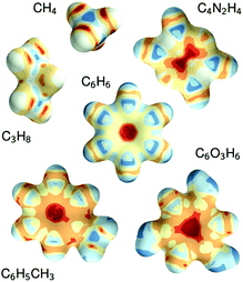 | ||
| Fig. 8 Chemical potentials for methane, propane, pyrazine, benzene, toluene, and phloroglucinol determined from SchNet.39 | ||
Returning to the Schrödinger equation (in Dirac notation),
| H|Ψn〉 = E|Ψn〉 |
where {|ϕi〉} is a set of N basis functions, and {ki} are the associated coefficients. Function |ϕi〉 can be an atom-centred Gaussian function. As a consequence, the electronic Schrödinger can be written in the matrix form
| Hkm = εmSkm |
| Hi,j = 〈ϕi|H|ϕj〉 |
| Si,j = 〈ϕi|ϕj〉 |
SchNOrb40 was developed to predict H and S using ML. The first part of the structure of SchNOrb is identical to SchNet in that it starts from initial representations of atom types and positions, continues with the construction of representations of chemical environments of atoms and atom pairs (again identical to the method used in SchNet) but then uses these to predict energy E and Hamiltonian matrix H, respectively.
The SchNet and SchNOrb systems illustrate how DNNs can be customized to specific scientific applications so that the DNN architecture promotes properties that are desirable in the data modelled by the network. Interpretation occurs by unpacking these networks. This strategy has already found success in several scientific areas including plasma physics41 and epidemiology.42 Another example is the use of a customised DNN43 to encode the hierarchical structure of a gene ontology to provide insight into the structure and function of a cell.
4 Discussion
We have briefly looked at the types of interpretable ML referred to in Fig. 4 and provided some chemical examples. In order to move forward, it is proposed that a research programme be designed that systematically compares the applicability and efficacy of the techniques over a wide range of chemical scenarios. The results of this exercise should be compiled into an on-line guide to support research (perhaps in an manner analogous to what was attempted for ML in the 1990s44). One of the existing Internet platforms for digital research collaboration might suffice.Roscher et al.27 divided the various forms of ML for scientific discovery into four groups. Group 1 includes approaches without any means of interpretability. With Group 2, a first level of interpretability is added by employing domain knowledge to design the models or explain the outcomes. Group 3 deals with specific tools included in the respective algorithms or applied to their outputs to make them interpretable, and Group 4 lists approaches where scientific insights are gained by explaining the machine learning model itself. These categories should help to structure the above proposed systematic comparison.
As regards the model-specific and model-agnostic approaches, it is anticipated that the agnostic method is more widely applicable because of the greater propensity of black-box systems.
The architectures of SchNet and SchNOrb are not learned but are designed with prior knowledge about the underlying physical process. In contrast, the aim of SciNet45 is to learn, without prior scientific knowledge, the underlying physics of a system from combinations of (a) observations (experimental data) taken from the physical system, (b) questions asked about the system, and (c) the correct answers to those questions in the context of the observations. This is done by attempting to use the latent neurons of an autoencoder network3 to learn and represent underlying physical parameters of the system. A network's learned representation is interpreted by analysing how the region of latent neurons responds to changes in the values of known physical parameters. For example, when given a time series of the positions of the Sun and the Moon, as seen from Earth, SciNet deduced Copernicus' heliocentric model of the solar system. This course to scientific discovery has not yet been applied to chemical systems but, given its potential, it is suggested that a clear methodology be developed that extends the SciNet-type approach to help chemists uncover new ideas and the links between them.
The exploration of the potential of interpretable ML to the sciences is growing, with applications in genomics,46 many-body systems,47 neuroscience48 and chemistry. Although this chemical review has focused on interpretation with respect to drug discovery and quantum chemistry, the potential of ML has been explored in other areas of chemistry, such as the use of ML for computational heterogeneous catalysis49 and retrosynthesis,50 and the use of interpretable ML in these and other fields is expected to prove to be immensely useful.
But a cautionary note. Reproducibility is fundamental to scientific research; thus, it is crucial that scientific discoveries arising from ML are reproducible, and this need must be factored into any methodology built for ML-based discovery. And the provision of raw research data with a publication is essential to overcome the “reproducibility crises”.51
In February 2020, the Alan Turing Institute held a workshop that announced the Nobel Turing Challenge; namely, “the production of AI systems capable of making Nobel-quality scientific discoveries highly autonomously at a level comparable, and possibly superior, to the best human scientists by 2050”. Chemistry is within the remit of the Challenge, and it is anticipated that interpretable ML will play a vital role toward the production of an ‘AI Chemist’.
Conflicts of interest
There are no conflicts to declare.Acknowledgements
We thank Pavlo Dral (Xiamen University) for discussions regarding Fig. 3, and Laurent Dardenne (DockThor), Thomas Unterthiner (Johannes Kepler University) and Alexandre Tkatchenko (University of Luxembourg) for permission to reproduce Fig. 2, 5, 7 and 8. We thank the Department of Chemistry, Cambridge University, for the Visiting Researchship. This work is dedicated to Zofia Kaczan-Aniecko.Notes and references
- S. Russell and P. Norvig, Artificial Intelligence: A Modern Approach, Pearson, Boston, 2010 Search PubMed.
- Induction: Processe of Inference, Learning and Discovery, ed. J. Holland, K. Holyoak, R. Nisbett and P. Thagard, MIT Press, Cambridge, MA, 1986 Search PubMed.
- I. Goodfellow, Y. Bengio and A. Courville, Deep Learning, MIT Press, Cambridge, MA, 2016 Search PubMed.
- K. Murphy, Machine Learning: A Probabilistic Perspective, MIT Press, 2012 Search PubMed.
- T. Hastie, R. Tibshirani and J. Friedman, The Elements of Statistical Learning, Springer, New York, 2nd edn, 2008 Search PubMed.
- C. Bishop, Neural Networks for Pattern Recognition, Clarendon Press, Oxford, 1995 Search PubMed.
- G. Goh, N. Hodas and A. Vishnu, 2017, arXiv, 1701.04503.
- Y. LeCun, Cognitiva, 1985, 85, 599–604 Search PubMed.
- D. Hubel and T. Wiesel, J. Physiol., 1962, 160, 106–154 CrossRef CAS.
- T. Cova and A. Pais, Front. Chem., 2019, 7, 809 CrossRef CAS.
- T. Xie and J. Grossman, 2017, arXiv, 1710.10324.
- M. Segler, M. Preuss and M. Waller, Nature, 2018, 555, 604–610 CrossRef CAS.
- Z. Zhou, X. Li and R. Zare, ACS Cent. Sci., 2017, 3, 1337–1344 CrossRef CAS.
- S. Smith, Nature, 2003, 422, 341–347 CrossRef.
- M. Lindsay, Nat. Rev. Drug Discovery, 2003, 2, 831–838 CrossRef CAS.
- S. Wang, T. Sim, Y.-S. Kim and Y.-T. Chang, Curr. Opin. Chem. Biol., 2004, 8, 371–377 CrossRef CAS.
- A. Lavecchia, Drug Discovery Today, 2015, 20, 318–331 CrossRef.
- A. Speck-Planche, V. Kleandrova, F. Luan and M. Cordeiro, Anticancer Agents Med. Chem., 2013, 13, 791–800 CrossRef CAS.
- I. Wallach, M. Dzamba and A. Heifets, 2015, ArXiv, 1510.02855.
- O. Trott and A. Olson, J. Comput. Chem., 2010, 31, 455–461 CAS.
- M. Mysinger, M. Carchia, J. J. Irwin and B. Shoichet, J. Med. Chem., 2012, 55, 6582–6594 CrossRef CAS.
- L. Chen, A. Cruz, S. Ramsey, C. Dickson, J. Duca, V. Hornak, D. Koes and T. Kurtzman, PLoS One, 2019, 14, e0220113 CrossRef CAS.
- T. Unterthiner, A. Mayr, G. Klambauer, M. Steijaert, J. Wegner, H. Ceulemans and S. Hochreiter, Deep Learning as an Opportunity in Virtual Screening, 2014, NIPS Workshop on Deep Learning and Representation Learning, Montreal, 12 December 2014.
- P. Dral, J. Phys. Chem. Lett., 2020, 11, 2336–2347 CrossRef CAS.
- M. Rupp, A. Tkatchenko, K.-R. Muller and O. A. von Lilienfeld, 2011, ArXiv, 1109.2618.
- P. Langley, H. Simon, G. Bradshaw and J. Zytkow, Scientific Discovery, MIT Press, Cambridge, MA, 1987 Search PubMed.
- R. Roscher, B. B. M. Duarte and J. Garcke, 2019, ArXiv, 1905.08883v2.
- L. Gilpin, D. Bau, B. Yuan, A. Bajwa, M. Specter and L. Kagal, 2019, ArXiv, 1806.00096v3.
- W. Murdoch, C. Singh, K. Kumbier, R. Abbasi-Asl and B. Yu, 2019, ArXiv, 1901.04592.
- A. Mahendran and A. Vedaldi, 2016, arXiv, 1512.02017.
- L. Breiman, J. Friedman, R. Olshen and C. Stone, Classification and Regression Trees, Chapman & Hall, New York, 1984 Search PubMed.
- F. Häse, I. Galván and M. Vache, Chem. Sci., 2019, 10, 2298 RSC.
- K. Preuer, G. Klambauer, F. Rippmann, S. Hochreiter and T. Unterthiner, 2019, ArXiv, 1903.02788v2.
- S. Bach, A. Binder, G. Montavon, F. Klauschen, K.-R. Muller and W. Samek, PLoS One, 2015, 10, e0130140 CrossRef.
- G. Goh, C. Siegel, A. Vishnu, N. Hodas and N. Baker, 2017, ArXiv, 1706.06689.
- S. Singh, M. Ribeiro and C. Guestrin, 2016, arXiv, 1602.04938.
- D. Nauck, F. Klawonn and R. Kruse, Foundations of Neuro-Fuzzy Systems, Wiley, Chichester, 1997 Search PubMed.
- L. Zadeh, Fuzzy Sets Syst., 1978, 1, 3–28 CrossRef.
- K. Schütt, F. Arbabzadah, S. Chmiela, K. Müller and A. Tkatchenko, 2016, ArXiv, 1609.08259v3.
- K. Schütt, M. Gastegger, A. Tkatchenko, K.-R. Müller and R. Maurer, Nat. Commun., 2019, 10, 5024 CrossRef.
- F. Matos, F. Hendrich, F. Jenko and T. Odstrcil, 82nd Annual Meeting of the DPG and DPG Spring Meeting of the AMOP Section, Friedrich Alexander University of Erlangen-Nuremberg, 2018.
- A. Adiga, C. Kuhlman, M. Marathe, H. Mortveit, S. Ravi and A. Vullikanti, Int. J. Adv. Eng. Sci. Appl. Math., 2018, 11, 153–171 CrossRef.
- J. Ma, M. Yu, S. Fong, K. Ono, E. Sage, B. Demchak, R. Sharan and T. Ideker, Nat. Methods, 2018, 15, 290–298 CrossRef CAS.
- Machine Learning: Neural and Statistical Classification, ed. D. Michie, D. Spiegelhalter and C. Taylor, Ellis Horwood, New York, 1994 Search PubMed.
- R. Iten, T. Metger, H. Wilming, L. Rio and R. Renner, 2018, ArXiv, 1807.10300v2.
- D. Sharma, A. Durand, M.-A. Legault, L.-P. L. Perreault, A. Lemaon, M.-P. Dub and J. Pineau, 2020, arXiv, 2007.01516.
- W. Zhong, J. Gold, S. Marzen, J. England and N. Halpern, 2020, arXiv, 2001.03623.
- A. Balwani and E. Dyer, bioRxiv, 2020 DOI:10.1101/2020.05.26.117473.
- A. Peterson, J. Chem. Phys., 2016, 145, 074106 CrossRef.
- M. Segler and M. Waller, Chem. – Eur. J., 2017, 23, 6118–6128 CrossRef CAS.
- T. Miyakawa, Mol. Brain, 2020, 13, 24 CrossRef.
| This journal is © The Royal Society of Chemistry and the Centre National de la Recherche Scientifique 2020 |

