ATR-FTIR spectroscopy coupled with chemometric analysis discriminates normal, borderline and malignant ovarian tissue: classifying subtypes of human cancer

Abstract

Surgical management of ovarian tumours largely depends on their histo-pathological diagnosis. Currently, screening for ovarian malignancy with tumour markers in conjunction with radiological investigations has a low specificity for discriminating benign from malignant tumours. Also, pre-operative biopsy of ovarian masses increases the risk of intra-peritoneal dissemination of malignancy. Intra-operative frozen section, although sufficiently accurate in differentiating tumours according to their histological type, increases operation times. This results in increased surgery-related risks to the patient and additional burden to resource allocation. We set out to determine whether attenuated total reflection Fourier-transform infrared (ATR-FTIR) spectroscopy, combined with chemometric analysis can be applied to discriminate between normal, borderline and malignant ovarian tumours and classify ovarian carcinoma subtypes according to the unique spectral signatures of their molecular composition. Formalin-fixed, paraffin-embedded ovarian tissue blocks were de-waxed, mounted on Low-E slides and desiccated before being analysed using ATR-FTIR spectroscopy. Chemometric analysis in the form of principal component analysis (PCA), successive projection algorithm (SPA) and genetic algorithm (GA), followed by linear discriminant analysis (LDA) of the obtained spectra revealed clear segregation between benign versus borderline versus malignant tumours as well as segregation between different histological tumour subtypes, when these approaches are used in combination. ATR-FTIR spectroscopy coupled with chemometric analysis has the potential to provide a novel diagnostic approach in the accurate diagnosis of ovarian tumours assisting surgical decision making to avoid under-treatment or over-treatment, with minimal impact to the patient.

---

Introduction

Ovarian cancer is the 5^th most common gynaecological cancer (incidence of 18 per 100 000) and the 4^th most common cause of cancer death (mortality of 8.8 per 10 000) in women in the UK.¹ In 2009, 5900 women were diagnosed with ovarian cancer; 3500 died from the disease the year after.² The high related mortality is a consequence of late presentation and diagnosis at stage III or IV resulting in five-year survival rates of 20% and 6%, respectively.²

Ovarian cancer encompasses a heterogeneous group of tumours, as indicated by differences in epidemiological and genetic risk factors, precursor lesions, patterns of spread, molecular events during oncogenesis, response to chemotherapy and prognosis.³ Ninety percent of ovarian cancers are malignant epithelial tumours termed carcinomas, the remainder being germ cell and sex cord-stromal tumours.⁴ The commonest types of ovarian carcinomas are high-grade serous carcinoma (HGSC), low-grade serous carcinoma (LGSC), mucinous carcinoma (MC), endometrioid carcinoma (EC), clear cell carcinoma (CCC), carcinosarcoma (CS) and mixed tumours (MT). Carcinomas are graded according to their cellular differentiation from normal tissue. This does not apply to HGSC and LGSC as they are considered different entities.⁵ Borderline epithelial tumours comprise approximately 15% of epithelial ovarian tumours and have a good prognosis. With the implementation of the “international classification of diseases for oncology (ICD-O-3)”, these tumours are no longer considered malignant.⁶

The complexity and heterogeneity of ovarian cancer with regards to risk factors, precursor lesions, morphological and clinical manifestations has hindered the development of robust population-based screening programs. Currently, in the UK, the assessment for ovarian cancer is based on “Risk Malignancy Index” (RMI 1 or 2), which encompasses menopausal status, ultrasonographic ovarian presentation and blood levels of the tumour marker Ca125 (see ESI Table S1†).^7,8 Other blood-derived biomarkers with similar accuracy to RMI have been suggested, for example HE4 and ROMA, but have not been established in practice.⁹ Also, magnetic resonance imaging (MRI), Doppler ultrasound and computed tomography (CT) have shown accuracies of 80% for the diagnosis of malignancy and 80–90% for the detection of abdominal spread.^10–12

Prognostic factors for ovarian cancer include stage and grade of cancer at diagnosis and residual disease after primary staging surgery.¹³ Histopathological tumour type is important when considering personalised treatment options. This plays a major role in chemotherapy responsiveness and therefore in overall survival rate.^13,14 For example, HGSC demonstrates much better response to platinum-based chemotherapy than CCC. This results in CCC having a lower 5-year survival than HGSC.¹⁵ It is obvious that current methods of ovarian cancer diagnosis and management have significant limitations. This is therefore a field that can benefit from research to identify novel methods of detecting and categorizing ovarian cancer to aid personalized intra- and post-operative management while also minimizing patient risk and resource expenditure.

Vibrational spectroscopy is a bio-analytical tool that has the potential to classify normal and pathological tissue according to their chemical and molecular differences.¹⁶ Complimentary techniques including Fourier-transform infrared (FTIR) and Raman spectroscopy have been utilised in the past few years to detect structural alterations that occur in molecules within cells according to their chemical bonds.^17–21 The resulting spectral differences may be used to distinguish benign from cancerous processes and classify cancer subtypes. Examples of areas studied by these methods include breast,²² endometrial,²³ cervical,²⁴ prostatic²⁵ and brain cancers.²⁶

We utilised ATR-FTIR spectroscopy to interrogate ovarian tissue harvested from women undergoing oophorectomies for several reasons including pelvic pain, postmenopausal bleeding, menorrhagia or dysfunctional uterine bleeding, premenstrual tension, risk reduction due to breast cancer or positive family history and imaging revealing ovarian cysts/masses. We hypothesized that spectrochemical analysis of ovarian tissue will allow diagnostic segregation of benign, borderline and cancerous tumours. Additionally, this method will allow classification of epithelial ovarian cancer subtypes. Resulting spectral datasets were analysed using multivariate analysis in the form of principal component analysis followed by linear discriminant analysis (PCA-LDA) and variable selection techniques in the form of successive projection algorithm (SPA) and genetic analysis (GA) again followed by LDA (SPA-LDA, GA-LDA). These chemometric techniques reduced the complexity of the spectral datasets and allowed visual representation. They were combined to form a classification machine. Additionally, we analysed our spectral datasets using multivariate control charts based on PCA²⁷ to examine whether biospectroscopy could correctly classify normal, borderline and cancerous ovaries.

Methods

Tissue collection and preparation

Ovarian specimens were acquired from the Royal Preston Hospital bio-bank with appropriate ethics clearance (REC reference 10/H0308/75). They included n = 35 histologically benign ovarian samples, n = 30 samples containing borderline ovarian tumours and n = 106 samples with a diagnosis of epithelial carcinoma. The ovarian carcinomas were further subdivided to HGSC (n = 46), LGSC (n = 9), EC (n = 15), MC (n = 12), CCC (n = 13), CS (n = 7) and MT (n = 4). Table 1 lists the specific histological diagnoses for these samples. The tissue samples were embedded in paraffin. Ten-μm-thick tissue sections were floated onto Low-E IR reflective slides (Kevley Technologies, Chesterland, OH, USA) slides. These were de-waxed by serial immersion in three sequential fresh xylene baths for 5 min and washed in an acetone bath for a further 5 min. The resulting samples were allowed to air dry and placed in a desiccator until analysis. Four-μm-thick parallel tissue sections were floated onto glass slides and stained with H&E for histological comparison, where needed.

Table 1 Histopathology of the ovarian tissues interrogated: Borderline tumours and malignant epithelial carcinomas are similarly staged according to FIGO Ovarian Cancer Staging 2014

Benign ovaries (n = 35)
Follicular cysts	Endometriosis	Involved in adhesions	Normal
2	2	2	29

---

Borderline ovaries (n = 30)
Stage/subtype	Serous	Sero-mucinous	Mixed epithelial
1a	10 (2× micro-invasion)	1	1
1b	1
1c	10
2a	1
3a	4 (1× micro-papillary)
3b	2 (1× micro-papillary)

---

Ovarian cancer (n = 109)
Stage/subtype	High-grade serous	Low-grade serous	Endometrial	Mixed ovarian tumour	Mucinous	Clear cell carcinoma	Carcino-sarcoma
1a	2	2	3		6	4
1b	1
1c	15	2	8		6	3	2
2a	2		2	1			1
2b				1
2c						1
3a	2		2	1		3
3b	5	2				1
3c	18	3		1		1	4
4	1

---

Classification of ovarian tissues according to histophathological characteristics

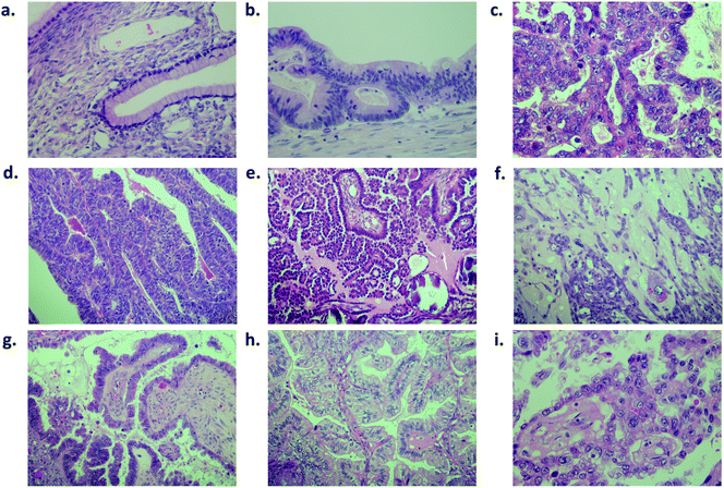
Fig. 1 shows a benign ovarian tumour (mucinous cystadenoma) (Fig. 1a), a borderline tumour (Fig. 1b) and different ovarian carcinoma subtypes stained (Fig. 1c–i) following H&E staining. The World Health Organization (WHO) criteria for classification of epithelial ovarian tumours are based on optical microscopy after H&E staining. They describe the tissues these carcinomas resemble and how they differ from each other in general terms. The WHO lists general criteria to assist the differentiation between the different subtypes (see ESI Table S2†).^28,29

Fig. 1 Benign and malignant ovarian tumour examples stained with H&E. (a) Mucinous cystadenoma (benign); (b) mucinous borderline tumour; (c) high-grade serous carcinoma; (d) endometrioid carcinoma; (e) low-grade serous carcinoma; (f) carcinosarcoma; (g) serous borderline carcinoma; (h) mucinous carcinoma; and, (i) clear cell carcinoma.

ATR-FTIR spectroscopy

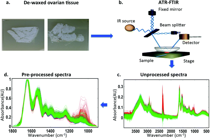
IR spectra were obtained using a Bruker Vector 27 FTIR spectrometer with a Helios ATR attachment containing a diamond crystal (≈250 μm × 250 μm sampling area) (Bruker Optics Ltd, Coventry, UK). Spectra were acquired from 10 randomly selected locations across the specimen to try and minimize bias by selection of areas with particular histopathological phenotype. A new background measurement was taken for every sample processed. The ATR crystal was cleaned with distilled water and dried with dry tissue paper before the acquisition of spectral background. The spectral resolution was 8 cm⁻¹ with 2× zero filling of the interferogram giving data spacing of 4 cm⁻¹. Spectra were co-added for 32 scans; these were converted into absorbance by Bruker OPUS software. Absorbance spectral images were converted to suitable digital files (.txt) for input to Matlab software.

Computational analysis

The ATR-FTIR datasets were processed using an in-house toolbox (iRootlab)³⁰ and PLS toolbox 7.8 (Eigenvector Research, Inc.3905 West Eaglerock Drive, Wenatchee, WA 98801) within a MATLAB R2014a environment (Mathworks Inc, Natick, MA, USA). The wavenumber regions inputted were between 4000 cm⁻¹ and 600 cm⁻¹. Spectra were then cut to include the regions between 1800–900 cm⁻¹. PCA-LDA reduces the complex spectral dataset into single points in hyperspace, while maximizing inter-class variation and minimizing intra-class variation. The disadvantage of this method is the potential over fitting of spectra causing arbitrary separation and therefore positive results. This can be counteracted by using large spectral datasets of more than five times the number of variables.

For the PCA-LDA, SPA-LDA and GA-LDA models, the samples were divided into training (70%), validation (15%) and prediction sets (15%) by applying the classic Kennard–Stone (KS) uniform sampling algorithm to the IR spectra.³¹ Training samples were used in the modelling procedure (including variable selection for LDA), whereas the prediction set was only used in the final evaluation of the classification. The optimum number of variables for SPA-LDA and GA-LDA was determined from the minimum cost function G calculated for a given validation dataset:

where g_n is defined asand I(n) is the index of the true class for the n^th validation object x_n.

The GA routine was carried out during 100 generations with 200 chromosomes each. Crossover and mutation probabilities were set to 60% and 10%, respectively. Moreover, the algorithm was repeated three times, starting from different random initial populations. The best solution (in terms of the fitness value) resulting from the three realizations of the GA was employed. For this study, LDA scores, loadings, and discriminant function (DF) values were obtained for the specimens. The first LDA factor (LD1) was used to visualize sample alterations in 1-dimensional (1D) score plots that indicate the main biochemical alterations.

Multivariate control charts were based on PCA. When the PCA model is applied on data collected when only common use variation is present, the future data behaviour can be referenced against this “in-control” model. In this sense, new multivariate observations can be projected onto the plane defined by the PCA loading vectors to obtain their scores (t_i,new = p^T_iy_new) and the residuals e_new = y_new − ŷ_new, where ŷ_new = P_AT_A,new, t_A,new is the (A × 1) vector of scores from the model and P_A is the (q × A) matrix of loadings. The presence of samples within the ±2 s control limits in the Shewhart control chart is built using the relevant PC scores. Trends and systematic behaviours in the scores plot are clear indications of “out-of-control” processes (i.e., normal ovarian tissue, borderline tissue and carcinoma subtypes).

Results

Classification of normal ovaries, borderline tumours and carcinomas

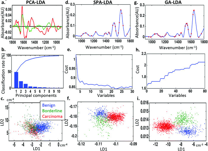
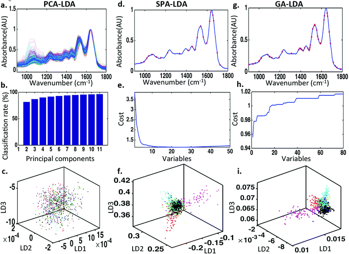
To discriminate between normal ovaries, ovaries with borderline tumours and those with carcinomas, the spectral dataset was pre-processed using 1^st order Savitzky–Golay smoothing (Order 2; Window 15) (Fig. 2). Overall, the IR spectra appear to overlap in the biochemical fingerprint region (1800 cm⁻¹ to 900 cm⁻¹). On closer inspection there are subtle but significant differences identified in the regions 1150–1000 cm⁻¹ (glycogen and nucleic acids), 1300–1200 cm⁻¹ (asymmetric phosphate stretching vibrations [ν_asPO₂⁻] and Amide III), 1550–1450 cm⁻¹ (protein moieties), 1600 to 1540 cm⁻¹ (Amide I region and DNA base region) and 1730–1630 cm⁻¹ (phospholipids and other lipids).

Fig. 2 Analysing ovarian tissues by ATR-FTIR spectroscopy and pre-processing resulting datasets. (a) 10 μm-thick ovarian tissue sections; (b) sample in close proximity with the ATR diamond; (c) unprocessed spectra; and (d) resulting spectra after pre-processing.

To examine these visible differences and attempt classification of the three categories, three types of chemometric analysis were used. Classification was achieved using PCA-LDA, SPA-LDA and GA-LDA. Seventy percent of the spectra were used to train the algorithm, 15% to test it internally and 15% to validate it externally (see ESI Table S3†). On comparing the spectra using PCA-LDA, seven PCs where used as this number provided significant classification (P < 0.001) without the introduction of arbitrary separation. Fig. 3c shows the 2-D scores plot derived by PCA-LDA. It reveals segregation of cancerous tissue from normal and borderline tumours, with the latter classes overlapping. The majority of differences between the normal and cancerous ovaries were attributed to Amide I (1674 cm⁻¹), nucleic acids (1620 cm⁻¹), different conformations of phenyl rings (1585 cm⁻¹, 1504 cm⁻¹), polysaccharides (1431 cm⁻¹) and symmetric phosphate stretching vibrations (ν_sPO₂⁻; 1096 cm⁻¹) (Fig. 3a). The chemometric technique that classified the three classes most successfully [66.4%] was GA-LDA using 29 variables determined from the minimum cost function G (Fig. 3g and h) (see ESI Table S4†). The related 2-D scores plot illustrates that spectral points from different classes dissociate while spectral points from the same class co-cluster (Fig. 3i). SPA-LDA also achieved considerable classification [55.9%] with separation of classes on a 2-D scores plot (Fig. 3f) when applied using 23 variables (Fig. 3d), again using the minimum cost function G (Fig. 3e) (see ESI Table S4†). All three techniques identified differences that aided classification within similar spectral regions. These differences were tentatively identified in the spectral regions of = 1400 cm⁻¹ (protein), = 1740 cm⁻¹ (lipid), = 1045 cm⁻¹ (phosphate), = 1545 cm⁻¹ (carbohydrate).

Fig. 3 Classification of benign, borderline and malignant ovarian tissue by spectral analysis using PCA-LDA, SPA-LDA and GA-LDA. (a) Loadings plot identifying the major discriminant wavenumbers for the three classes; x-axis is cm⁻¹ and the y-axis represents absorbance coefficient. The five wavenumbers contributing to the most segregation were derived from the points furthest away from the x-axis. (b) Cost/function plot identifying the optimal number of PCs to be used for PCA. (c) Scores plot graphically representing classification by PCA-LDA; x-axis represents LD1 and the y-axis LD2. (d) Wavenumber selection for SPA-LDA. (e) Cost/function plot identifying the optimal number of wavenumbers to be used for the SPA algorithm. (f) Scores plot graphically representing classification by SPA-LDA; x-axis represents LD1 and the y-axis LD2. (g) Wavenumber selection for GA-LDA. (h) Cost/function plot identifying the optimal number of wavenumbers to be used for the GA algorithm. (i) Scores plot graphically representing classification by GA-LDA; x-axis represents LD1 and the y-axis LD2 (red = cancer, green = borderline, blue = benign).

Lipid-to-protein ratio, phosphate-to-carbohydrate ratio and RNA-to-DNA ratio

To further evaluate the importance of the above spectral regions in classifying the ovarian tumours to benign, borderline and malignant specimens, intensity ratios of spectral areas important for classification were measured (Table 2).

Table 2 Statistical significance of classification of normal, borderline and malignant ovarian tumours based on ratios of lipid-to-protein, phosphate-to-carbohydrate and RNA-to-DNA spectral intensities. Statistical significance was calculated using one-way ANOVA followed by Tukey's test

Classes/ratios	Lipid-to-protein ratio	Phosphate-to-carbohydrate ratio	RNA-to-DNA ratio
Normal vs. cancer	P < 0.0001	P < 0.0001	P < 0.0001
Normal vs. borderline	P > 0.5	P < 0.0001	P < 0.0001
Borderline vs. cancer	P < 0.0001	P < 0.0001	P > 0.5

---

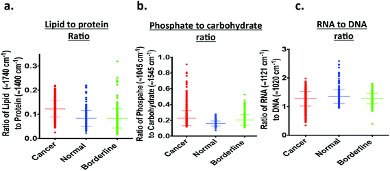
Fig. 4a shows the lipid-to-protein ratio, which is obtained by calculating the ratio of band intensities at 1750 cm⁻¹ to 1730 cm⁻¹ (lipids) and 1410 cm⁻¹ to 1390 cm⁻¹ (protein). The lipid-to-protein ratio was higher in neoplastic tissue and lower in borderline and benign tissue (Table 2). Normal and benign tissue exhibited similar ratios. The parameters used for the tentatively-assigned phosphate-to-carbohydrate ratio in each IR spectrum were derived from the intensity of phosphate at 1055 cm⁻¹ to 1045 cm⁻¹ and of carbohydrate at 1555 cm⁻¹ to 1535 cm⁻¹. The phosphate-to-carbohydrate ratio is mildly increased in ovarian carcinomas relative to borderline and benign tissue and the difference is also significant (P < 00001) (Fig. 4b; Table 2). When comparing the intensity ratios of RNA (1111 cm⁻¹ to 1131 cm⁻¹) to DNA (1010 cm⁻¹ to 1030 cm⁻¹), the ovarian carcinomas exhibited slightly lower ratios (Fig. 4c).

Fig. 4 Classification of ovarian tumours to benign, borderline and malignant using spectral intensity ratios. (a) Intensity ratio of lipid-to-protein; (b) intensity ratio of phosphate-to-carbohydrate; and, (c) intensity ratio of RNA-to-DNA.

Classification of normal ovaries, ovaries with borderline tumours and those with ovarian carcinoma using multivariate control charts based on PCA

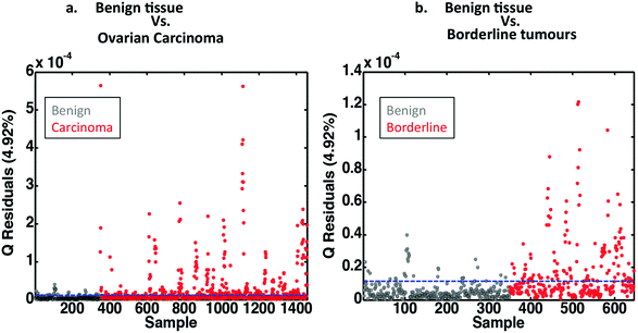
Multivariate control charts are commonly used in industry for quality control of chemical substances. A similar approach may be used in biospectroscopy. Tissue from benign ovaries can act as “control tissue” against which borderline and neoplastic tissues are compared. The control is represented by a line at zero, and another line is drawn usually at two standard deviations (SDs). How far from normal this line is from zero depends on the variability that exists within the examined tissue. When comparing borderline and malignant tissue with benign control tissue everything outside the SD lines is considered abnormal. Interestingly, control charts, derived from the PCA already performed are able to distinguish between normal and neoplastic ovaries (Fig. 5a) and normal and those with borderline tumours (Fig. 5b).

Fig. 5 Classification of ovarian tumours to benign, borderline and malignant using Shewhart control charts after PCA. (a) Benign ovarian tissue vs. malignant tissue; and, (b) benign ovarian tissue vs. borderline tissue.

Classification of carcinoma subtypes using PCA-LDA, SPA-LDA and GA-LDA

Similar chemometric techniques have been used to classify epithelial ovarian carcinomas according to their subtypes. The aforementioned pre-processing of the spectral datasets was applied in this case also. Seven PCs were used for PCA (Fig. 6b), 23 wavenumbers for SPA (Fig. 6d) and 44 wavenumbers for GA (Fig. 6g) (see ESI Table S5†). The number of wavenumbers to be used was again determined by the minimum cost function G (Fig. 6e and h). PCA, SPA and GA followed by LDA were not adequately successful when comparing the spectral datasets of all cancer subtypes together as revealed by the associated 3-D scores plots (Fig. 6c, f and i). There was however visible separation between clear cell carcinoma (cyan), carcinosarcoma (pink) and high-grade serous carcinoma (blue) subtypes when analysed SPA-LDA and separation between clear cell carcinoma (cyan), carcinosarcoma (pink) spectral classes when analysed by GA-LDA. Unfortunately there was not adequate visual separation between classes with PCA-LDA.

Fig. 6 Classification of ovarian carcinoma subtypes by spectral analysis using PCA-LDA, SPA-LDA and GA-LDA. (a) Pre-processed spectral dataset. Each colour represents a particular neoplastic subtype. (b) Cost/function plot identifying the optimal number of PCs to be used for PCA. (c) Scores plot graphically representing classification by PCA-LDA; x-axis represents LD1 and y-axis LD2. (d) Wavenumber selection for SPA-LDA. (e) Cost/function plot identifying the optimal number of wavenumbers to be used for the SPA algorithm. (f) Scores plot graphically representing classification by SPA-LDA; x-axis represents LD1 and y-axis LD2. (g) Wavenumber selection for GA-LDA. (h) Cost/function plot identifying the optimal number of wavenumbers to be used for the GA algorithm. (i) Scores plot graphically representing classification by GA-LDA; x-axis represents LD1 and y-axis LD2 (blue = high grade serous, red = low grade serous, black = endometrioid carcinoma, yellow = mixed, green = mucinous, cyan = clear cell, pink = carcinosarcoma).

Two-category discriminant analysis of carcinoma subtypes using PCA-LDA, SPA-LDA and GA-LDA

To increase the classification success rate, spectral datasets representing different epithelial tumour subtypes were compared in pairs. The three chemometric techniques previously mentioned where utilised again. Similar validation methods were used with 70% of the data being used to train the system, 15% for internal validation and 15% for external validation. The optimum number of PCs for PCA and variables for SPA-LDA and GA-LDA was determined by power versus cost calculation using the minimum cost function G (see ESI Fig. S1†). ESI Fig. S2–S4† represent graphically the 2-D scores plots derived by PCA-LDA, SPA-LDA and GA-LDA, respectively, following comparison of all the carcinoma subcategories after ATR-FTIR spectroscopy. The three analytical techniques were not equally successful at distinguishing between the categories compared. Fig. 7 presents the percentage success for classification with each method. In general, distinguishing between the different carcinoma subclasses was more successful when using GA-LDA.

Fig. 7 Percentage successful classification of ovarian carcinoma subtypes when compared in pairs using three chemometric analyses: PCA-LDA, SPA-LDA, GA-LDA. Red boxes represent the most successful technique for each particular pair analysed. Amber colour represents the second most successful technique and green the least.

Discussion

Our study demonstrates that ATR-FTIR spectroscopy in conjunction with powerful chemometric approaches has the potential to distinguish between normal, borderline and neoplastic ovarian tissue. It also has the potential to distinguish between different ovarian epithelial carcinoma subtypes. The most conspicuous differences are between normal ovaries and overt carcinoma, identified by the chemometric techniques employed. This finding is significant due to its potential for translation into clinical practice. Currently, histological identification is the gold standard in the diagnosis of ovarian cancer and therefore essential for surgical decision-making. Benign ovarian masses do not require extensive surgery, while ovarian carcinomas will usually be managed by “staging” surgery involving a bilateral salpingooopherectomy, hysterectomy, omentectomy and pelvic lymphadenectomy. Pre-operative biopsy methods have been suggested to obtain histological diagnosis before embarking in major surgery. For example, image-guided fine needle aspiration cytology (FNAC) and core biopsy using ultrasound, CT or MRI imaging have been shown to be effective with a diagnostic accuracy of 80.9% and 93% respectively.^32,33

These diagnostic modalities are usually preserved for women with co-morbidities that prohibit primary staging surgery or where imaging has revealed potentially inoperable disease. The reason for this is the risk of upstaging the disease by causing intra-peritoneal spillage of cancerous cells. Where there is a high clinical suspicion of ovarian cancer, a “staging procedure” is performed, which includes bilateral salpingo-oopherectomy, hysterectomy, omentectomy and pelvic lymphadenectomy.

In cases where clinical suspicion alone is not enough to embark on staging surgery, intra-operative consultation by a pathologist is pursued. This utilises “frozen section” of the specimen, which is then stained, usually with H&E, and is examined by optical microscopy. Frozen section distinguishes benign from malignant tumours very accurately, but is less accurate for borderline tumours.^34,35 It prevents morbidity associated with surgical staging procedures in benign cases and under-treatment of malignant tumours, which would otherwise require restaging surgery or chemotherapy. Frozen section has several limitations that include sampling difficulties, interpretation errors and communication breakdown.³⁶ It also causes increases in surgical times, with resultant morbidity to the patient. ATR-FTIR spectroscopy in conjunction with chemometric analysis allows the identification of biomarkers that can be adapted for easy discrimination between benign and neoplastic tissue during surgery. Indeterminate ovarian masses that would otherwise require a frozen section may be processed. The processing of ovarian tumour samples may be performed in an area adjacent to an operating theatre using desktop ATR spectroscopy instruments or even within an operating theatre, using handheld devices. In our experiment the spectral dataset for each sample was acquired in approximately seven minutes (approximately 1 second per scan, 32 scans for each of 10 areas). The remaining time was spent readjusting the stage to a different area within the sample. Our spectral analysis was performed in a stepwise manner, therefore timing for the analysis is difficult to estimate. Our in-house tools for matlab, irootlab^30,37,38 can be adjusted to analyse spectral datasets using analysis cascades that would complete the procedure within minutes, reducing surgical duration. They would also require minimal operator training. Spectral datasets of control tissue could be pooled retrospectively and used for the calibration of the different analyses performed and increase accuracy of the tests.³⁹ For example multivariate control charts may be used to distinguish malignant ovarian tumours that would require extensive surgery from benign or borderline tumours that will not.

The clinical importance for the diagnosis of ovarian carcinoma subtypes lays with their implications in immediate and subsequent management, medical or surgical, their follow-up and genetic counselling. Patients with early-stage (1a) mucinous or endometrioid carcinoma can be treated with surgery alone. Patients with high-grade serous carcinoma will routinely have adjuvant chemotherapy. Those with mucinous, endometrioid, and clear cell carcinomas may have adjuvant or neo-adjuvant combination radiotherapy and chemotherapy. High-grade serous adenocarcinoma is also associated with BRCA mutations; therefore, patients may be referred for genetic testing and if proven positive their families would be screened. ATR-FTIR spectroscopy coupled with a chemometric machine has the potential of being adopted as an additional tool for pathological interpretation of ovarian carcinomas.

Conclusion

The purpose of this study was to identify spectral differences within ovarian tissues with the capability of classifying them in accordance to their histopathological status. Utilising ATR-FTIR spectroscopy, n = 171 ovarian tissues were examined. Morphological and molecular alterations within these tissues have already been associated with neoplasia. Spectroscopic analysis of these tissues reveals specific alterations linked to malignancy. The responsible changes for this segregation were primarily alterations in the tentatively-assigned lipid (1740 cm⁻¹)-to-protein (1400 cm⁻¹) ratio, with a marked increase associated with carcinomas. IR spectroscopy coupled with chemometric analysis has the potential to differentiate not only neoplastic from borderline and benign tissues but also distinguish between different carcinoma subtypes. Further validation of these approaches exploiting other biospectroscopy techniques and using larger and architecturally more robust datasets is required.

Acknowledgements

Thanks to Lancashire Teaching Hospitals NHS Trust and Rosemere Cancer Foundation for funding these studies.

References

1. CancerStats Ovarian cancer-UK, Cancer Research UK, 2011.
2. National Cancer Intelligence Network, 2012.
3. J. Prat, Ann. Oncol., 2012, 23(Suppl 10), x111–117.
4. Surface epithelial-stromal tumours, in World Health Organisation Classification of Tumours: pathology and genetics of tumours of the breast and female genital organs, ed. F. A. Tavassoli and P. Devilee, 2003, pp. 117–145.
5. J. Prat, Virchows Arch., 2012, 460, 237–249.
6. I. Cadron, F. Amant, T. Van Gorp, P. Neven, K. Leunen and I. Vergote, Curr. Opin. Oncol., 2006, 18, 488–493.
7. I. Jacobs, D. Oram, J. Fairbanks, J. Turner, C. Frost and J. G. Grudzinskas, BJOG, 1990, 97, 922–929.
8. S. Tingulstad, B. Hagen, F. E. Skjeldestad, M. Onsrud, T. Kiserud, T. Halvorsen and K. Nustad, BJOG, 1996, 103, 826–831.
9. M. A. Karlsen, N. Sandhu, C. Hogdall, I. J. Christensen, L. Nedergaard, L. Lundvall, S. A. Engelholm, A. T. Pedersen, D. Hartwell, M. Lydolph, I. A. Laursen and E. V. Hogdall, Gynecol. Oncol., 2012, 127, 379–383.
10. E. K. Outwater, E. S. Siegelman, K. M. Wilson and D. G. Mitchell, Radiology, 1996, 200, 483–488.
11. M. R. Buist, R. P. Golding, C. W. Burger, J. B. Vermorken, P. Kenemans, E. M. Schutter, J. P. Baak, M. A. Heitbrink and T. H. Falke, Gynecol. Oncol., 1994, 52, 191–198.
12. D. L. Brown, M. C. Frates, F. C. Laing, D. N. DiSalvo, P. M. Doubilet, C. B. Benson, E. D. Waitzkin and M. G. Muto, Radiology, 1994, 190, 333–336.
13. J. L. Brun, A. Feyler, G. Chene, J. Saurel, G. Brun and C. Hocke, Gynecol. Oncol., 2000, 78, 21–27.
14. T. Sugiyama, T. Kamura, J. Kigawa, N. Terakawa, Y. Kikuchi, T. Kita, M. Suzuki, I. Sato and K. Taguchi, Cancer, 2000, 88, 2584–2589.
15. A. du Bois, H. J. Luck, W. Meier, H. P. Adams, V. Mobus, S. Costa, T. Bauknecht, B. Richter, M. Warm, W. Schroder, S. Olbricht, U. Nitz, C. Jackisch, G. Emons, U. Wagner, W. Kuhn, J. Pfisterer and G. Arbeitsgemeinschaft Gynakologische Onkologie Ovarian Cancer Study, J. Natl. Cancer Inst., 2003, 95, 1320–1329.
16. F. L. Martin, Nat. Methods, 2011, 8, 385–387.
17. M. J. Baker, J. Trevisan, P. Bassan, R. Bhargava, H. J. Butler, K. M. Dorling, P. R. Fielden, S. W. Fogarty, N. J. Fullwood, K. A. Heys, C. Hughes, P. Lasch, P. L. Martin-Hirsch, B. Obinaju, G. D. Sockalingum, J. Sule-Suso, R. J. Strong, M. J. Walsh, B. R. Wood, P. Gardner and F. L. Martin, Nat. Protoc., 2014, 9, 1771–1791.
18. H. Y. Holman, M. C. Martin, E. A. Blakely, K. Bjornstad and W. R. McKinney, Biopolymers, 2000, 57, 329–335.
19. M. Jackson, M. G. Sowa and H. H. Mantsch, Biophys. Chem., 1997, 68, 109–125.
20. J. R. Mourant, Y. R. Yamada, S. Carpenter, L. R. Dominique and J. P. Freyer, Biophys. J., 2003, 85, 1938–1947.
21. E. Taillandier and J. Liquier, Methods Enzymol., 1992, 211, 307–335.
22. J. G. Kelly, A. A. Ahmadzai, P. Hermansen, M. A. Pitt, Z. Saidan, P. L. Martin-Hirsch and F. L. Martin, Anal. Bioanal. Chem., 2011, 401, 957–967.
23. S. E. Taylor, K. T. Cheung, I. I. Patel, J. Trevisan, H. F. Stringfellow, K. M. Ashton, N. J. Wood, P. J. Keating, P. L. Martin-Hirsch and F. L. Martin, Br. J. Cancer, 2011, 104, 790–797.
24. K. Gajjar, A. A. Ahmadzai, G. Valasoulis, J. Trevisan, C. Founta, M. Nasioutziki, A. Loufopoulos, M. Kyrgiou, S. M. Stasinou, P. Karakitsos, E. Paraskevaidis, B. Da Gama-Rose, P. L. Martin-Hirsch and F. L. Martin, PLoS One, 2014, 9, e82416.
25. M. J. Baker, E. Gazi, M. D. Brown, J. H. Shanks, N. W. Clarke and P. Gardner, J. Biophoton., 2009, 2, 104–113.
26. K. Gajjar, L. D. Heppenstall, W. Pang, K. M. Ashton, J. Trevisan, I. I. Patel, V. Llabjani, H. F. Stringfellow, P. L. Martin-Hirsch, T. Dawson and F. L. Martin, Anal. Methods, 2012, 5, 89–102.
27. F. S. L. Costa, R. H. P. Pedroza, D. L. Porto, M. V. P. Amorim and K. M. G. Lima, J. Braz. Chem. Soc., 2015, 26, 64–73.
28. V. W. Chen, B. Ruiz, J. L. Killeen, T. R. Cote, X. C. Wu and C. N. Correa, Cancer, 2003, 97, 2631–2642.
29. N. Lalwani, S. R. Prasad, R. Vikram, A. K. Shanbhogue, P. C. Huettner and N. Fasih, Radiographics, 2011, 31, 625–646.
30. J. Trevisan, P. P. Angelov, A. D. Scott, P. L. Carmichael and F. L. Martin, Bioinformatics, 2013, 29, 1095–1097.
31. R. W. Kennard and L. A. Stone, Technometrics, 1969, 11, 137–148.
32. G. Mehdi, V. Maheshwari, S. Afzal, H. A. Ansari and M. Ansari, J. Cytol., 2010, 27, 91–95.
33. J. A. Spencer, K. Anderson, M. Weston, N. Wilkinson and M. Hewitt, Cancer Imaging, 2006, 6, 144–147.
34. J. L. Brun, A. Cortez, R. Rouzier, P. Callard, M. Bazot, S. Uzan and E. Daraï, Am. J. Obstet. Gynecol., 2008, 199, 244.e1–244.e7.
35. L. R. Medeiros, D. D. Rosa, M. I. Edelweiss, A. T. Stein, M. C. Bozzetti, A. Zelmanowicz, P. R. Pohlmann, L. Meurer and M. T. Carballo, Int. J. Gynecol. Cancer, 2005, 15, 192–202.
36. H. Jaafar, Malays. J. Med. Sci., 2006, 13, 4–12.
37. J. Trevisan, P. P. Angelov, P. L. Carmichael, A. D. Scott and F. L. Martin, Analyst, 2012, 137, 3202–3215.
38. N. C. Purandare, I. I. Patel, K. M. G. Lima, J. Trevisan, M. Ma'Ayeh, A. McHugh, G. Von Bünau, P. L. Martin Hirsch, W. J. Prendiville and F. L. Martin, Anal. Methods, 2014, 6, 4576–4584.
39. A. L. Mitchell, K. B. Gajjar, G. Theophilou, F. L. Martin and P. L. Martin-Hirsch, J. Biophoton., 2014, 7, 153–165.

---

Footnote

† Electronic supplementary information (ESI) available. See DOI: 10.1039/c5an00939a

---