
 Open Access Article
 This Open Access Article is licensed under a Creative Commons Attribution-Non Commercial 3.0 Unported Licence
The Alaska permanent fund dividend increases residential payments for water services†
Barbara
Johnson
 *a,
Allen
Molina
b,
Mark
Herrmann
d and
Srijan
Aggarwal
*ce
*a,
Allen
Molina
b,
Mark
Herrmann
d and
Srijan
Aggarwal
*ce
aDepartment of Natural Resources and Environment, University of Alaska Fairbanks, 99775, Fairbanks, Alaska, USA. E-mail: bajohnson20@alaska.edu
bOregon Department of Transportation, 97301, Salem, Oregon, USA. E-mail: allen_molina@ymail.com
cCivil, Geological, and Environmental Engineering Department, University of Alaska Fairbanks, 99775, Fairbanks, Alaska, USA. E-mail: saggarwal@alaska.edu
dCollege of Business and Security Management, University of Alaska Fairbanks, 99775, Fairbanks, Alaska, USA. E-mail: mlherrmann@alaska.edu
eWater and Environmental Research Center, Institute of Northern Engineering, University of Alaska Fairbanks, Fairbanks, 99775, Alaska, USA
First published on 30th November 2023
Abstract
Alaska has the lowest rate of access to in-home water services in the United States. At the same time, the state also has the world's oldest Universal Basic Income (UBI) program, and every Alaska resident receives an annual payment through the Alaska Permanent Fund Dividend (PFD) program. In this study, we use a panel dataset of rural Alaska water and sewer utilities in 18 Alaska villages from 2012 to 2016 to explore the impact of the PFD on residential payments. We estimate fixed effects for eight models. Models are developed by grouping villages by low and high variability in payments, enrollment in Alaska Native Claims Settlement Act (ANCSA) regional corporations and Community Development Quota (CDQ) organizations. We find that on average, each utility is missing $14![[thin space (1/6-em)]](https://www.rsc.org/images/entities/char_2009.gif) 710 in customer payments yearly, and have a median residential delinquency rate of 14%. The model with all the villages (p < 0.01), ANCSA models (p < 0.05), and CDQ models (p < 0.05) all show a significant increase in residential payments when the PFD is paid in October. Average residential payments in October are $3671 to $10058 higher than in other months. The increased payments represent 2% to 6% of the total revenue of utilities. We estimate that across rural Alaska the PFD generates between $734200 to $2011600 in additional payments for water utilities. These findings suggest that the PFD and other unrestricted cash transfers can play an important role in increasing household water security in rural Alaska and other places with similar problems.
710 in customer payments yearly, and have a median residential delinquency rate of 14%. The model with all the villages (p < 0.01), ANCSA models (p < 0.05), and CDQ models (p < 0.05) all show a significant increase in residential payments when the PFD is paid in October. Average residential payments in October are $3671 to $10058 higher than in other months. The increased payments represent 2% to 6% of the total revenue of utilities. We estimate that across rural Alaska the PFD generates between $734200 to $2011600 in additional payments for water utilities. These findings suggest that the PFD and other unrestricted cash transfers can play an important role in increasing household water security in rural Alaska and other places with similar problems.
Environmental significanceThe ability of water and wastewater utilities to provide public health and environmental benefits requires generating enough revenue to cover their operations and maintenance (O&M) costs. O&M are typically covered from user revenue, and rising O&M result in higher costs for consumers. Already, across the United States, access to in-home water services is hindered by affordability and the problem is expected to worsen. Universal Basic Income (UBI) may help increase water security by increasing household income. This paper uses the Alaska Permanent Fund Dividend – the longest-running UBI – to explore the impact of UBI on water services. We find that households increase their payments for water services in October, when they receive their PFD. |
Introduction
There is fear that Artificial Intelligence (AI) will increase unemployment and decrease incomes.1–3 While the impact of AI is still unknown, an increase in unemployment would affect water security. Already, over 10% of American households struggle to pay their water bills,4 and rising operating costs are expected to increase the number of households with unaffordable bills to 35%.5 AI has brought attention to Universal Basic Income (UBI),6,7 a recurring payment to an entire population with no spending restrictions.8 UBIs could improve access to water services since affordability is a function of both price and household disposable income.9–11 We explore this relationship by looking at Alaska which has the lowest access to water services in the United States12 and the world's oldest UBI,13 the Alaska Permanent Fund Dividend (PFD).Started in 1982, the PFD is funded by the investment of oil and gas royalties. Every year, the PFD is paid in October to every Alaska resident. The nominal value of payments has ranged from $331 in 1984 to $3284 in 2022.14 UBIs and other unrestricted cash transfers decrease poverty.15–17 Studies in urban areas found that UBIs increase consumption.18,19 In a poll of 1023 Americans, 13% of respondents indicated they would use a UBI to pay for utilities.20 In California, households participating in a pilot UBI project spent 10% ($50 per month) of their UBI on utility bills.21 Yet, to our knowledge, no peer-reviewed study has examined the impact of UBIs on payments for utilities. This work fills a literature gap by exploring the impact of the PFD on payment for water services in rural Alaska.
Today, only 78% of rural Alaska households have in-home plumbing22 compared to 99.6% nationally,23 resulting in higher rates of diseases.22,24–26 Most villages are off-the-road system, and only accessible by plane or boat, resulting in high transportation costs and costs of living. Village economies are a mix of subsistence and cash generating activities, with a strong informal (unreported trade of services and goods) sector.27 The remote location is due to colonial policies which resulted in the creation of permanent settlements without any planning.28,29 Thirty-two villages have no plumbing and must self-haul their drinking water and waste.30 In plumbed villages, access is limited by breakdowns and high operating costs31,32 and unaffordable user bills.33,34
This work examines the impact of the PFD on payment for piped water services using a monthly panel dataset of 18 villages in rural Alaska from 2012 to 2016. The PFD is paid in October, and the amount varies yearly. We exploit the dataset's spatial and temporal variation to isolate the PFD's impact on household payments for water services while controlling for the village and time-fixed effects. In our analysis, we also control for villages' enrollment in Community Development Quota (CDQ) groups and with an Alaska Native Claims Settlement Act (ANCSA) corporation.
Methods
ANCSA and CDQs
Alaska Native Claims Settlement Act (ANCSA) corporations are important political and economic entities in Alaska and are often involved in infrastructure development. In 1971, ANCSA conveyed 44 million acres of land to the newly established 12 regional and over 200 village for-profit corporations.35 ANCSA settled long-standing Alaska Native claims settlement issues, allowing the development of the North Slope oil fields. ANCSA corporations distribute dividends to their shareholders, invest in their respective regions, and provide financial assistance to their shareholders.36 In 2021, ANCSA regional corporations had between $232 million and $3.9 billion in revenue.37 Nonetheless, the median household income in eight ANCSA regions is lower than the state average, and seven regions have a lower plumbing access (ESI Table 1†).12 ANCSA corporations publicly release little information about dividends beyond the amount per share.15The Western Alaska Community Development Quota (CDQ) program is another important economic actor. Established in 1998, the CDQ program created six non-profit economic development CDQ groups to manage fisheries quota on behalf of eligible villages, previously excluded from the fisheries due to privatization.38 The CDQ groups receive royalties from fishing quotas and must facilitate economic development in member villages.38 While CDQ groups cannot pay out dividends they can and do provide energy subsidies and scholarships and invest in infrastructure development,39 which can increase the disposable income of households. Per the most recent estimate available, the CDQ groups spend between $1787 and $80131 per resident.40 As such, there is potentially some direct or indirect effect on water security.
Data
We use a panel constructed from the 2012–2016 accounting records of water and sewer utilities (“water utilities”) and publicly available socioeconomic data. The water utilities are enrolled in a program that helps with administrative tasks, purchases, and maintenance. The utilities must meet specific criteria to join and remain in the program. The names of the program and water utilities are withheld for privacy reasons. We exclude 10 water utilities from the panel. Of these, six are excluded to avoid small samples biasing the results. We define a small sample as fewer than 90 people in the village or a utility having 20 or fewer residential customers. It is likely that in every village every month at least one household (residential customer) is late paying their bill for a variety of reasons. A single missing payment can be significant in small villages (one household is 5% of 20 households) but would be insignificant in larger villages. While there is not a universal definition of what constitutes a small sample and setting thresholds is somewhat arbitrary41 there is evidence that a sample size of at least 25 is sufficient to identify variability.42 Since payments for water services are at the household level, we set a threshold so that all included villages have an average of 25 households at a minimum. We exclude two water utilities that received subsidies of unknown amounts as the subsidies are recorded as residential payments and would bias the results. We also exclude two water utilities with missing socioeconomic data. All dollar values are inflation-adjusted to January 2022. The descriptive statistics are shown in Table 1. Boxplots showing the inter-annual variations are included in the supplementary section (ESI Fig. 1–6†).| Min | Max | Mean | Median | Stand. dev. | |
|---|---|---|---|---|---|
| Water | |||||
| Residential rate ($/month) | $69.78 | $310.09 | $153.32 | $142.59 | $51.29 |
| Customers | 29 | 136 | 74.33 | 71 | 32.39 |
| Residential collection rate | 0.00% | 544.65% | 89.53% | 83.67% | 39.91% |
| Residential payment($/month) | $0 | $59321.52 |
$10028 |
$7309.13 | $7783.55 |
| Commercial revenue ($/month) | $-836.63 | $128300 |
$2257.59 | $1075.43 | $5605.22 |
| School revenue ($/month) | $-3421.97 | $26115.72 |
$4452.99 | $3951.72 | $3783.93 |
|
|||||
| Electricity | |||||
| Price ($/kW h) | $0.53 | $1.13 | $0.74 | $0.74 | $0.09 |
| PCE ($/kW h) | $0.27 | $0.84 | $0.48 | $0.48 | $0.08 |
| Household costs ($/month) | $48.59 | $896.98 | $177.1 | $157.60 | $71.80 |
|
|||||
| Demographics | |||||
| Population | 93 | 876 | 421.57 | 383 | 233.68 |
| Households | 23 | 197 | 95.67 | 98 | 45 |
| Household size | 2.85 | 5.69 | 4.36 | 4.41 | 0.68 |
|
|||||
| Employment | |||||
| Labor force participation | 66.13% | 113.36% | 88.20% | 89.05% | 10.42% |
| Employment rate | 63.85% | 85.54% | 76.05% | 75.90% | 5.07% |
| Unemployment rate | 14.45% | 36.14% | 23.94% | 24.09% | 5.07% |
|
|||||
| Income | |||||
| Household wage ($/house) | $694.02 | $6242.42 | $2844.77 | $2764.84 | $920.56 |
| Wage per capita | $191.05 | $1668.13 | $674.71 | $644.70 | $219.67 |
| PFD/person | $1057 | $2410 | $1631 | $1427 | $578 |
| PFD/village | $102308 |
$1771264 |
$676618 |
$585550 |
$442223 |
|
|||||
| Environmental | |||||
| Temperature (°C) | −35.57 | 25.90 | −0.71 | −0.89 | 10.91 |
Again, there are significant differences between villages.43 Employment levels vary between 64% and 86%, unemployment ranges from 14% to 36%, and labor participation rates are between 66% and 113%. It is unclear why some rates are above 100%, and this is likely due to data collection issues in rural Alaska.15 Monthly household wages range from $694 to $6242, with a median of $2845. The annual PFD payments range from $1057 to $2410 per person (Fig. 1).14 The villages receive between $102308 and $1771264 in total PFD payments, depending on their population.
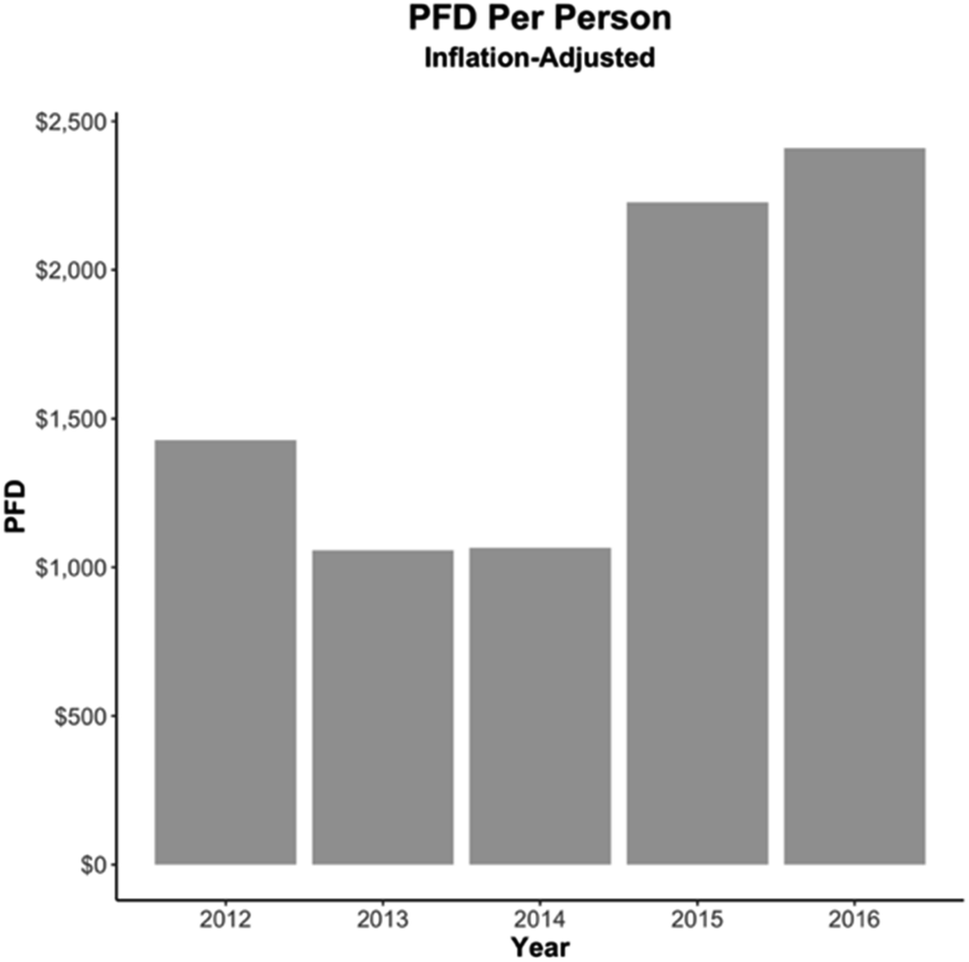 | ||
| Fig. 1 Annual PFD payment during the period of study. | ||
Payments to the water utilities vary monthly and yearly. The utilities record payments in the month they are received, regardless of whether customers pay current, or past bills, or pre-pay. Six utilities recorded $0 in residential customer payments in one or more months for a total of 10 observations which are included in the analysis to avoid bias in the data. The residential collection rate (amount paid over amount billed) ranges from 0% to 545%, and monthly residential payments range from $0 to $59321 with a mean of $10028. Schools and commercial entities are also customers of the water utilities. Monthly school payments range from −$3422, to $26116 and commercial payments range from −$837 to $128300.
The dataset includes residential electricity costs to account for changes in the costs of living in the villages. The electricity data is obtained from the Alaska Energy Authority (AEA) Power Cost Equalization (PCE) database.44 The PCE is a State of Alaska program that subsidizes the first 500 kW h consumed by rural households every month.44 Subsidized rates range from $0.27/kW h to $0.85/kW h with a median of $0.48/kW h, about four times higher than the national average.45 The average monthly residential electricity costs are computed using the following equation:
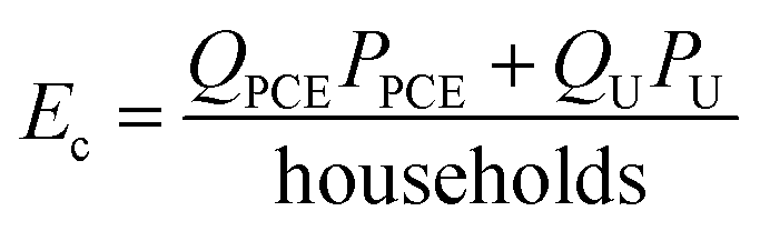 | (1) |
Electricity bills are lagged by a month, with households paying for the previous month's consumption. PPCE is the subsidized price of electricity ($/kW h), QPCE is the amount of subsidized electricity (kW h) consumed by all households in the previous month, PU ($/kW h) is the unsubsidized price of electricity and QU (kW h) is the unsubsidized amount consumed in the previous month. We divide by the number of households to calculate the average per-household cost (Ec). The household electricity costs range from $49 to $897, with an average cost of $177. These costs account for 1.4% to 21% of household wages, with an average burden of 6%.
Empirical approach
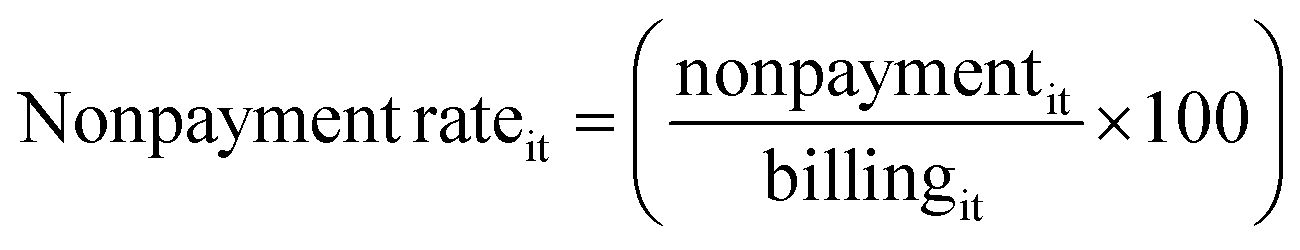
The underlying assumption of this study is that several residential customers struggle to pay their water bills. We start by determining whether the annual and monthly billing amounts exceed payments:| nonpaymentict = billingict − paidict | (2) |
 | (3) |
We study the impact of PFD on residential payments for water and sewer bills using a fixed effects model. Since the PFD is paid in October, we expect that month's residential payments to be higher. A basic model of the fixed effects estimates is:
| yit = β1xit + ai + μit | (4) |
Hence, the fixed effects models the impact of the PFD on residential payments within each village and at each period. The variable a is the fixed effect of each village – a set of unobserved characteristics within each village that may mediate the impact of independent variables like the PFD. To isolate the impact of the PFD, we must control for the variability within each village (individual heterogeneity). The fixed effect transformation controls for individual heterogeneity by time-demeaning the data through differencing where the average of the model over time is subtracted from each period:
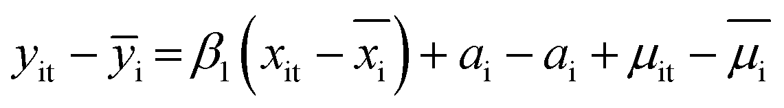 | (5) |
The transformation results in the unobserved characteristics (a) being zeroed out and disappearing from the model. Differencing also zeroes out time-invariant variables such as location and ANCSA corporation.41 Therefore, the changes in residential payments (dependent variable) must be due to the independent variables remaining in the model after differencing, which vary over time.47
We adapt the methodology of Watson et al. (2020)48 and estimate the coefficients for the following empirical model:
| Payit = β0 + β1Mit + β2Yit + β3Pit+ β4Ecit + β5Sit + β6Ct + β7Hit + β8HWit + β9Tit + ai + μit | (6) |
As before, i denotes the villages, and t is the month and year (time period) the observation occurred in. Each utility in the dataset is located in a different village. Pay is the dependent variable and is the total residential payments a utility receives in a time period. Month (M) and year (Y) time effects are included to control for the timing of the PFD and other unexpected events.41 The residential rate (P) controls for changes in the price of water services which could impact residential demand and payments. The household cost of electricity (Ec) is the average household electricity bill and is a proxy for living costs. The model includes payments for water services from schools (S) and commercial entities (C) as indicators of differences in billing and administration within and between utilities. H is the number of households in the village, since water services are provided per household, and HW is the average household wage. Finally, the model includes monthly average temperature (T) data to account for environmental factors, such as a prolonged cold spell that could decrease household income or cause systems to freeze.
The time-fixed effects estimates are calculated about a base month and year. When October is the base month, the coefficients of the other months are the difference in payments received compared to October, so we can quantify the additional payments received. The fixed effect estimates are generated using STATA version 17 (ref. 49) and the user-built xtscc50 and xtt3 (ref. 51) packages. The Hausman test confirms that fixed effects are appropriate (p < 0.01). We use Driscoll-Kraay standard errors since the Breausch-Pagan LM test of independence and modified Wald statistics test are significant (p < 0.01), indicating the presence of cross-sectional dependence and heteroskedasticity.52
The key assumption underlying this empirical approach is that the PFD is the only regular but non-monthly payment to occur in October, which to our knowledge is the case. Nonetheless, we want to account for the possibility that there may be other factors, such as ANCSA dividends, or fuel subsidies in CDQ villages, occurring in October. To do this, we estimate fixed effects for eight models. In Model 1, estimates are generated for the entire panel dataset. To explore whether certain villages with higher variability in residential payments in October bias the fixed effects estimates in Model 1, we group the villages by low (Model 2) and high variation (Model 3). To categorize villages by variation in residential payments, we calculate average October z-score for each village and set the low and high threshold as the median z-score (1.56) across all villages.
We also split the villages by ANCSA corporation and enrollment in a CDQ group to further explore how unknowns may impact the October fixed effects estimates. In Models 4–6 we group villages by ANCSA corporation. Each corporation is independent, and they issue dividends and other assistance at different times. If an ANCSA corporation issues a payment we are unaware of in October, these models should capture that. In Model 4, the villages' ANCSA corporation issues its dividend in April, while in Model 5 the other ANCSA corporation's dividends are issued in February, June and/or December, depending on the year. In Model 6, we aggregate four villages which are enrolled with three different ANCSA corporations to obtain a panel large enough to generate fixed effect estimates. The corporations in this model pay their dividends in March, September, or December. We use a similar approach to explore the possible impact of CDQ groups. Fixed effects estimates are generated in Model 7 for the eleven villages not part of CDQ groups, and in Model 8 for the seven CDQ villages. We aggregate the CDQ villages in a single model as there is insufficient data to generate estimates for each CDQ group.
Lastly, we calculate the share of the PFD captured by water utilities by again, using an approach similar to Watson et al. (2020)48 by estimating fixed effects for the following:
| Payit = β0 + β1PFDTotit + β2PFDTotit2 + ai+ μit | (7) |
Results and discussion
PFD and residential payments
It is clear from the estimated equations (Table 2) that the residential payments in October, when the PFD is issued, are significantly higher than in other months (Fig. 2). This finding holds for the aggregated model (model 1) as well as when villages are disaggregated by the size of the October variance from the average month (models 2 and 3), by when the ANCSA corporate dividend is paid (models 4 to 6) and whether the village is part of a CDQ group (models 7 and 8). These are very robust findings in that the October payments are significantly higher than in any other month for all the eight models considered here, with most p-values 0.01.| What impacts residential payments? | Variation | ANCSA-corporation dividend | CDQ | |||||
|---|---|---|---|---|---|---|---|---|
| (1) All villages | (2) Low | (3) High | (4) April | (5) Feb, June, Dec | (6) March & Sep, Dec | (7) Non-CDQ | (8) CDQ | |
| a ***(p < 0.01), **(p < 0.05), *(p < 0.1). | ||||||||
| Month (base = Oct) | ||||||||
| January | −7210.29*** | −2503.48** | −12056.36*** |
−5221.93*** | −8832.34*** | −14799.47*** |
−5651.47*** | −11691.02*** |
| February | −5403.81*** | −2474.21** | −8330.14*** | −5472.74*** | −6706.68*** | −9248.26*** | −4449.82*** | −8425.25*** |
| March | −4645.08*** | −2532.94** | −7371.76*** | −3718.82*** | −7537.74*** | −8447.74** | −4975.17*** | −6350.37** |
| April | −6291.85*** | −3889.64*** | −8994.70*** | −4444.29*** | −7161.39*** | −12077.63*** |
−5185.84*** | −9467.80*** |
| May | −7456.35*** | −4627.87*** | −10786.18*** |
−6352.41*** | −6708.74*** | −12516.61*** |
−4990.62*** | −12305.77*** |
| June | −6768.12*** | −4143.52*** | −9750.12*** | −6452.40*** | −4688.27*** | −10178.69*** |
−4297.89*** | −11158.17*** |
| July | −6096.36*** | −4248.98*** | −7557.75*** | −5166.73*** | −4400.36** | −6233.08*** | −3753.04*** | −8107.10*** |
| August | −6540.13*** | −4405.28*** | −8007.79*** | −5451.65*** | −4898.85*** | −7298.68*** | −4212.18*** | −8245.85*** |
| September | −6477.64*** | −4703.00*** | −8007.68*** | −5423.59*** | −6351.39*** | −7062.01*** | −4575.36*** | −8089.37*** |
| November | −6742.70*** | −2811.45* | −10439.02*** |
−4589.13*** | −8471.72*** | −11398.28*** |
−5562.15*** | −9427.55*** |
| December | −7033.54*** | −4037.08*** | −10057.66*** |
−5158.61*** | −9582.53*** | −11378.53*** |
−5936.59*** | −9904.33*** |
|
||||||||
| Year (base = 2012) | ||||||||
| 2013 | 1128.10** | 1124.33* | 1558.42*** | 633.91 | 3757.74*** | −519.69 | 1812.95*** | 632.77 |
| 2014 | 1778.43*** | 2440.50*** | 1557.99*** | 300.13 | 5585.84*** | 522.74 | 2970.83*** | 982.35 |
| 2015 | 755.19 | 886.97 | 994.74* | 152.08 | 2385.32** | −163.20 | 1050.76* | 1461.10* |
| 2016 | 692.51* | 988.90 | 970.86* | −366.13 | 1566.12 | −383.17 | 1050.82** | 1124.63 |
|
||||||||
| Public utilities | ||||||||
| Residential (P) | 29.08** | 28.19 | 35.00*** | 11.55 | 38.46 | 47.75** | 28.74** | 42.98** |
| School pay (S) | 0.30*** | 0.52*** | 0.13** | 0.13*** | 0.60*** | 0.09 | 0.48*** | 0.07 |
| Commercial (C) | 0.04** | 0.02 | 0.07* | −0.03 | 0.12* | 0.07* | 0.05 | 0.05 |
| Electr. cost (Ec) | 3.85 | 0.49 | 3.11 | 19.49*** | 0.09 | −8.35 | −1.17 | 10.36** |
|
||||||||
| SocioEcon | ||||||||
| Households (H) | 12.27 | −5.14 | −40.99 | 22.86 | −81.25** | −61.57 | −65.74** | −75.97 |
| Household wage (HW) | −0.01 | 0.84** | −3.12*** | −2.96* | 1.16*** | −5.68*** | 0.56* | −6.50*** |
| Temperature (T) | 18.18 | 82.20* | −53.61 | 111.27** | −107.16 | −193.43 | −37.20 | 31.63 |
| Prob > F | 0.000 | 0.000 | 0.000 | 0.000 | 0.000 | 0.000 | 0.000 | 0.000 |
| Within-R2 | 0.2006 | 0.2029 | 0.3056 | 0.2731 | 0.3431 | 0.2491 | 0.2499 | 0.2941 |
| Observations | 1020 | 510 | 510 | 444 | 336 | 240 | 636 | 384 |
| Villages | 18 | 9 | 9 | 8 | 6 | 4 | 11 | 7 |
 | ||
| Fig. 2 We normalize the monthly revenue from residential payments by dividing each month's average residential revenue by the average residential revenue in October for each model (a)–(h). This results in October always being 1. To convey the differences in residential payments between the models we include the total value of residential payments in October in yellow. | ||
The increase in residential payments differs across villages and months. The average difference in payments between October and other months varies between $3671 (Model 2) and $10058 (Model 6). Taking the average across all the models, we find that October residential payments are $6961 higher (per village). Since the median annual revenue of the utilities in the panel is $168847, the additional residential payments in October account for 2% to 6% of total annual revenue. To extrapolate these results to the all rural water utilities across Alaska, we multiply the range of estimated excess October residential water payments by 200 (∼number of villages) to suggest that the PFD generates between $734200 to $2011600 in additional payments every year.
Our findings complement the existing studies on cash transfers and household consumption. They are consistent with Kueng (2015),19 which found that the PFD increases urban consumption. One difference is that unlike Kueng (2018),18 we found that the impact of the PFD on water and sewer utilities is restricted to October and does not extend to November and December. Other studies have also found that household consumption increases with cash transfers53–55 and households in a UBI pilot program in California spent 10% of the UBI on utility services.21 Lower-income households spend a higher proportion of their cash transfer on non-durable goods such as food and on paying off debt56–59 which is consistent with our results.
Payments by schools and commercial entities
Recall that we included payments for water services from schools (S) and commercial entities (C) as indicators of differences in billing and administration within and between utilities. We theorized that billing practices impact customer payments and would vary by model. A $1 increase in school payments is associated with a statistically significant increase in residential payments between $0.13 (Model 3 and 4, p < 0.05 and p < 0.01) and $0.60 (Model 5, p < 0.01). School payments are not significant in Models 6 and 8. Commercial payments also positively affect residential payments, however, generally with smaller effects. A $1 increase in commercial payments is only associated with an increase in residential payments between $0.04 (Model 1, p < 0.05) and $0.12 (Model 5, p < 0.1) in Models 1,3, 5, and 6 and is not statistically significant in the others. This may be explained by commercial rates being structured differently than rates for residents and schools.Missing payments and delinquency rates
Since customer payments account for almost the entirety of the utilities' revenue, missing payments hinder the ability of utilities to perform maintenance and repairs.33 We estimate that the 18 utilities are missing $264770 in customer payments every year. This works out to $14710 per utility, or approximately one month of revenue ($14070) and an overall delinquency rate of 7%. Residential bills account for 97% of the unpaid amount. Since the PFD is associated with an average increase in payments of $6961, we infer that without the PFD the average unpaid amount would be $21670. Hence, the PFD reduces missing payments by just over 30%.
The value of the unpaid bills and the delinquency rates vary across time and by customer group (Fig. 3 and ESI Table 3†). The 2012–2016 delinquency rate is 11% (median of 14%) for residential customers, 0% for commercial entities and 1% for schools, which indicates that over time, commercial and school bills are paid in full but not residential ones. As expected, residential delinquency rates are lowest in October (p < 0.01), when the residential delinquency rate averages −36% (overpayment), compared to 15% in the other months. Notably, October is the only month when residential delinquency rates are negative. Residential delinquency rates peak November through January and in May (average of 19%). Cash-generating activities vary seasonally,27 which may explain why residential payments vary seasonally. The commercial delinquency rate in October is like the rate in January, April and June (p > 0.1) and it is slightly lower than in the other months (p < 0.1). While we have no explanation for these variations, we hypothesize that they are linked to the businesses cash flow. The schools' October delinquency rate is not significantly different than in other months (p > 0.1).
 | ||
| Fig. 3 Monthly variation in unpaid bills for water services by type of customer. The yellow dots are the month of October. | ||
Residential water rates
The water utilities must balance setting a price their customers are able to pay and generating enough revenue to cover their operating costs. This can be an impossible balancing act. Like other small utilities in the countries, these utilities have a small customer base over which to distribute their high costs.60–62 There are few alternatives to rate revenue. The State of Alaska only sporadically provides funding for operations and maintenance costs and the Indian Health Service is the only federal agency permitted to fund operations costs, but Congress has never appropriated the funding.33Nonetheless, residential water rates only have a moderate effect on residential payments in our models. Water rates are not significant in Models 2, 4, and 5. In the other models, a $1 increase in residential rates is associated with an increase in village payments of $29–$48 (p < 0.5 to p < 0.01). To better investigate the impact of residential rates, we estimate the random effects for the models and report the results in ESI Table 4.† Random effects examine drivers of differences between villages.41 The random effect estimates for residential rates are significant in all the models, indicating that their moderate effect in the fixed effects models may be a statistical anomaly due to the rates remaining relatively constant across the years (ESI Fig. 4†).
Cost of electricity
Electricity costs are included as a proxy for costs of living as there is no other village-level data for this. In our models, electricity is only significant in models 4 and 8. A $1 increase in household electricity expenditure is associated with an approximate increase of $19 in residential payments in Models 4 (p < 0.01) and $10 in Model 8 (p < 0.5). Electricity costs may be a poor indicator of changes in costs of living, or they may not change significantly in the period of study. In the random effects model, the electricity costs account for differences in residential payments in three models (p < 0.05).Water and electricity burden
We hypothesize that the effect of the PFD is linked to the affordability of water bills and costs of living. In rural Alaska, costs are high. In 2020, the average cost of electricity was $0.60/kW h,63 compared to a national average of 0.14/kW h.45 In our panel, households spend between 5% to 50% of their wages just on water, sewer, and electricity, for an average burden of 12%, almost twice the national average for household expenditure on all utilities.64 In this context, it is unsurprising that even the higher-income villages experience an increase in payments with cash transfers, highlighting the extent of the affordability issue across rural Alaska. These problems are expected to worsen as the operating costs of utilities are increasing.32,65Household income and PFD
The PFD represents a substantial proportion of household income. From 2012 to 2016, the PFD accounted for 11.6% of the average annual household income of the 18 villages in the panel. During that same period, the PFD accounted for 4.3% of the average annual household income in Alaska (Fig. 4). The difference is likely because although the villages have different economies, all have high costs of living and few formal employment opportunities.27,66,67 In addition, cash-generating activities often conflict with subsistence, of which it is hard to overstate the importance.28,68–70 | ||
| Fig. 4 PFD as a percentage of annual household income in Alaska and in the dataset (18 villages). | ||
Wages
The impact of wages (earned income) varies by model. Household wages are not statistically significant in the combined model and have a contrasting impact in the other models. In Models 3, 5, and 7, a $1 increase in household wage results in an increase in residential payments between $0.6 (Model 7, p < 0.1) and $1.2 (Model 5, p < 0.01). In models 3, 4, 6, and 8, a $1 increase in household wages is associated with a decrease in residential payments between $3.1 (Model 3, p < 0.01) and $6.5 (model 8, p < 0.01). Again, we refer to the random effects estimate (ESI Table 3†) to better understand the role of household wages. Household wages are only significant in four models and again have opposite signs.The negative effect between household wages and residential payments in some models is somewhat surprising. These results may be due to using wage data, which excludes unearned income (e.g. PFD or social security), or to the assumptions used to decompose the wages to the monthly level. Another reason may be seasonality, although we would expect the time-fixed effects to remove time trends. Nonetheless, we notice that household wages are over $1200 higher in the summer (ESI Table 5†), and there is no significant increase in residential payments. Summer is also an important time for subsistence. We hypothesize that households prioritize subsistence activities, which are intrinsic both to Indigenous ways of life28,69,70 and food security.68 Engaging in subsistence requires purchasing equipment and fuel71,72 and costs vary by village. For example, CDQ villages (Model 8) are coastal villages with a tradition of traveling onto the ocean to fishing,73,74 which may entail higher costs compared to inland villages.
Share of the PFD
We estimate that residential customers spend 1.4–2.6% of their PFD on water services (p < 0.01, Table 3). The average total PFD amount received in each village is $676618, with $9472 (1.4% of PFD payments, Table 3) of that going to the water utility. If only 55% of the population is connected, they would receive $372140 in PFD payments. We find that on average a water utility would receive $9676 (2.6% of PFD, Table 3 payments). Both these figures are slightly higher than the previously estimated average increase in payments of $6961 but are within the previously estimated range of $3671–$10058. The disparity is likely due to the different approaches used.
| What share of each PFD dollar is paid to water utilities? | % of population connected to the water utility | |
|---|---|---|
| 100% | 55% | |
| a ***(p < 0.01), **(p < 0.05), *(p < 0.1). | ||
| PFDTot | 0.014*** | 0.026*** |
| PFDTot2 | −4.63 × 10⁻⁹ | −1.53 × 10⁻⁸ |
| Prob > F | 0.000 | 0.000 |
| Within-R2 | 0.1486 | 0.1486 |
Informal economy
These findings are particularly relevant to communities with a significant informal economy and limited formal employment opportunities. A benefit of UBIs like the PFD is that they reach everyone, including workers in the informal economy.75 Broadly defined, an informal economy is the unreported trade of goods and services that may or may not involve cash exchanges.27,76 The informal economy accounts for a large but unquantified proportion of the rural Alaska economy,27,77,78 30% of the global GDP79 and 8% of the American GDP.76 The ubiquity of the informal economy around the world makes our findings relevant to communities outside of Alaska.Limitations
It is important to consider the limitations of this study. The statistical analysis does not establish a causal relationship between the PFD and increased residential payments. This could be a spurious relationship resulting from their interaction with unaccounted variables.80 Another limitation stems from the lack of household level data. We disaggregate village-level data which may obscures differences in household behavior. Given these data limitations, we cannot control for the impact of outlier households on our results. Taken together, these limitations may explain the inconsistent impact of wages and electricity costs on residential payments. The impact of household wages may be underestimated as the data does not include unearned income and transfer payments can account for a significant proportion of household income.15 Finally, we lack data on the number of households who are customers of the water utility. In addition, the data does not allow us to distinguish between back payments, payments for current bills and pre-payments. Given this, we are unable to estimate some useful metrics, such as how many households are delinquent. These results would also be strengthened by a study of other unrestricted cash transfers, like ANCSA dividends and tax refunds.Conclusion
Our findings suggest that the PFD plays an important role in household water security and helping utilities cover their costs in rural Alaska. We find that, on average, each water utility is missing $14710 annually in payments from all customers. The median residential delinquency rate is 14%. Residential payments increase significantly in October, when the PFD is received by households. October residential payments are on average $6961 higher than in other months. In the panel, the increased payments represent between 2% and 6% of the total revenue of utilities. We estimate that annually the PFD results in $734200 to $2011600 in additional payments across rural Alaska and decreases missing revenue by almost 40%.
The PFD appears to play an important role in both ensuring household access to water services and helping utilities recoup their costs. These findings are contextualized within the discussion of affordability. We find that on average the households in the panel dataset spend 12% of their income on water and electricity, which is almost twice the national average for household expenditure on all utilities. In some villages, we estimate that water and electricity accounts for half of the average household income. This situation is exacerbated by a limited number of cash-generating opportunities. This issue of affordability is not unique to rural Alaska. Across the country, an increasing number of households struggle to pay their utility bills.
In addition to the growing affordability crisis, there are increasing fears of mass unemployment due to AI. Based on the results of this study, we find that the PFD and other UBIs and unrestricted cash transfers may be effective tools to enhance household access to basic services, increasing water security.
Author contributions
Barbara Johnson: conceptualization, methodology, software, data curation, visualization, writing–original draft preparation, writing-review and editing. Dr Allen Molina: data curation, software, visualization, writing-original draft preparation. Dr Mark Herrmann: software, writing-original draft preparation, writing-review and editing. Dr Srijan Aggarwal: methodology, data curation, visualization, supervision, writing-original draft preparation, writing-review and editing.Conflicts of interest
There are no known conflicts to declare.Acknowledgements
This work was supported by a United States Geological Survey (USGS) National Institute for Water Resources (NIWR) graduate student grant # 2019AK014BReferences
- Q. P. Nguyen and D. H. Vo, Artificial intelligence and unemployment: An international evidence, Struct. Chang. Econ. Dyn., 2022, 63, 40–55 CrossRef.
- M. Mutascu, Artificial intelligence and unemployment: New insights, Econ. Anal. Policy, 2021, 69, 653–667 CrossRef.
- A. Korinek, and J. E. Stiglitz, Artificial Intelligence and its Implications for Income Distribution and Unemployment, University of Chicago Press, 2018 Search PubMed.
- D. S. Cardoso and C. J. Wichman, Water affordability in the United States, Water Resour. Res., 2020, 58(12) DOI:10.1029/2022WR032206.
- E. A. Mack and S. Wrase, A burgeoning crisis? A nationwide assessment of the geography of water affordability in the United States, PLoS One, 2017, 12(1) DOI:10.1371/journal.pone.0169488.
- M. Walker, BIG and technological unemployment: Chicken Little versus the economists, J. Eth. Emerg. Tech., 2014, 24, 5–25 CrossRef.
- A. Agrawal, J. Gans and A. Goldfarb, Economic policy for artificial intelligence, Innov. Policy Econ., 2019, 19, 139–159 CrossRef.
- M. S. Kearney and M. Mogstad, Universal basic income (UBI) as a policy response to current challenges, Report, Aspen Institute, 2019, pp. 1–19 Search PubMed.
- J. Mugabi, S. Kayaga, I. Smout and C. Njiru, Determinants of customer decisions to pay utility water bills promptly, Water Policy, 2010, 12, 220–236 CrossRef.
- Y. B. Zaied, M. Kertous, N. B. Cheikh and B. B. Lahouel, Delayed payment of residential water invoice and sustainability of water demand management, J. Clean. Prod., 2020, 276, DOI:10.1016/j.jclepro.2020.123517.
- B. E. Akinyemi, A. Mushunje and A. E. Fashogbon, Factors explaining household payment for potable water in South Africa, Cogent Soc. Sci., 2018, 4(1) DOI:10.1080/23311886.2018.1464379.
- US Census Bureau, American Community Survey 5-year ACS Demographic and Housing Estimates, 2012-2021, https://data.census.gov/table?q=demographics+and+housing+estimates%26tid=ACSDP1Y2021.DP05 Search PubMed.
- E. W. De Barbieri, Purchasing population growth, Ind. LJ, 2022, 98, 575–622 Search PubMed.
- Alaska Department of Revenue, Summary of Dividend Applications & Payments, https://pfd.alaska.gov/Division-Info/Summary-of-Applications-and-Payments, accessed June 2023 Search PubMed.
- M. Berman, Resource rents, universal basic income, and poverty among Alaska's Indigenous peoples, World Dev., 2018, 106, 161–172 CrossRef.
- D. Salehi-Isfahani, B. Wilson Stucki and J. Deutschmann, The Reform of Energy Subsidies in Iran: The Role of Cash Transfers, Emerg. Mark. Finance Trade, 2015, 51, 1144–1162 CrossRef.
- S. B. Patel and J. Kariel, Universal basic income and covid-19 pandemic, Br. Med. J., 2021, 372, 1756–1833, DOI:10.1136/bmj.n193.
- L. Kueng, Excess sensitivity of high-income consumers, Q. J. Econ., 2018, 133, 1693–1751 CrossRef.
- L. Kueng, Expected Permanent Fund Dividends: New Measures Based on a Narrative Analysis and Archival Data, SSRN, 2015 DOI:10.2139/ssrn.2746483.
- Skynova, What would you do on UBI?, https://www.skynova.com/blog/what-would-you-do-on-ubi, accessed 2023 June.
- Stockton Economic Empowerment Demonstration, Preliminary Analysis: SEED's First Year, Report, 2020, https://www.stocktondemonstration.org/s/SEED_Preliminary-Analysis-SEEDs-First-Year_Final-Report_Individual-Pages.pdf Search PubMed.
- L. Eichelberger, S. Dev, T. Howe, D. L. Barnes, E. Bortz, B. R. Briggs, P. Cochran, A. D. Dotson, D. M. Drown, M. B. Hahn, K. Mattos and S. Aggarwal, Implications of inadequate water and sanitation infrastructure for community spread of COVID-19 in remote Alaskan communities, Sci. Total Environ., 2021, 776, 145842, DOI:10.1016/j.scitotenv.2021.145842.
- US Census Bureau, American Community Survey 5-year ACS Demographic and Housing Estimates, https://data.census.gov/table?q=demographics+and+housing+estimates%26tid=ACSDP1Y2021.DP05, accessed January 2023 Search PubMed.
- T. W. Hennessy, T. Ritter, R. C. Holman, D. L. Bruden, K. L. Yorita, L. Bulkow, J. E. Cheek, R. J. Singleton and J. Smith, The relationship between in-home water service and the risk of respiratory tract, skin, and gastrointestinal tract infections among rural Alaska natives, Am. J. Public Health, 2008, 98, 2072–2078, DOI:10.2105/ajph.2007.115618.
- K. A. Hickel, A. Dotson, T. K. Thomas, M. Heavener, J. Hébert and J. A. Warren, The search for an alternative to piped water and sewer systems in the Alaskan Arctic, Environ. Sci. Pollut. Res., 2018, 25, 32873–32880 CrossRef PubMed.
- T. Thomas, K. Hickel and M. Heavener, Extreme water conservation in Alaska: limitations in access to water and consequences to health, Public Health, 2016, 137, 59–61 CrossRef CAS PubMed.
- O. S. Goldsmith, The Remote Rural Economy of Alaska, Institute of Social and Economic Research, University of Alaska Anchorage, 2007 Search PubMed.
- C. B. Stern, PhD thesis, From Camps to Communities: Neets'ąįį Gwich'in Planning and Development in a Pre- and Post-Settlement Context, University of Alaska Fairbanks, 2018 Search PubMed.
- G. Berardi, Schools, settlement, and sanitation in Alaska Native villages, Ethnohistory, 1999, 46, 329–359 Search PubMed.
- Alaska Department of Environmental Conservation, Alaska Water and Sewer Challenge (AWSC), https://dec.alaska.gov/water/water-sewer-challenge/, accessed 2023 January Search PubMed.
- L. Eichelberger, K. Hickel and T. K. Thomas, A community approach to promote household water security: Combining centralized and decentralized access in remote Alaskan communities, Water Security, 2020, 10, 100066, DOI:10.1016/j.wasec.2020.100066.
- M. Rashedin, B. Johnson, S. Dev, E. Whitney, J. Schmidt, D. Madden and S. Aggarwal, Rural Alaska Water Treatment and Distribution Systems Incur High Energy Costs: Identifying Energy Drivers Using Panel Data Analysis for 78 Communities, ACS ES&T Water, 2022, 12, 2668–2676 Search PubMed.
- Alaska Department of Environmental Conservation, A Framework to Assess the Affordability of Residential Water and Sewer Rates in Rural Alaska, Report, 2020, https://dec.alaska.gov/media/21759/alaska-w-and-s-affordability-model-report.pdf Search PubMed.
- Kawerak, Kawerak Inc – Public Coment on BIA Tribal Transportation Program, 2015, https://www.regulations.gov/comment/BIA-2014-0005-0004 Search PubMed.
- ANCSA Regional Association, About the Alaska Native Claims Settlement Act, https://ancsaregional.com/about-ancsa/, accessed 2023 January Search PubMed.
- ANCSA Regional Association, Economic Impacts, https://ancsaregional.com/economic-impacts/, accessed January 2023 Search PubMed.
- Alaska Business, Top 49ers - 2022https://www.akbizmag.com/2022-top49ers/, accessed June 2023 Search PubMed.
- C. Lyons, C. Carothers and J. Coleman, Alaska’s community development quota program: A complex institution affecting rural communities in disparate ways, Marine Policy, 2019, 108, 103560 CrossRef.
- NOAA, The Western Alaska Community Development Quota, Report, NOAA, 2018, https://media.fisheries.noaa.gov/dam-migration/cdq-program-summary-1018.pdf Search PubMed.
- Coastal Villages Region Fund, Annual Report, Report, 2012, https://issuu.com/kk_coastalvillages/docs/2012_annual_report Search PubMed.
- J. M. Wooldridge, Econometric Analysis of Cross Section and Panel Data, The MIT Press, 2010 Search PubMed.
- D. G. Jenkins and P. F. Quintana-Ascencio, A solution to minimum sample size for regressions, PLoS One, 2020, 15, e0229345 CrossRef CAS PubMed.
- Alaska Department of Labor, Employment and Wages Data for All Locations, 2001 to 2016, https://dcra-cdo-dcced.opendata.arcgis.com/datasets/employment-and-wages-2001-to-2016-all-locations, accessed January 2023 Search PubMed.
- Alaska Energy Authority, Power Cost Equalization, Report, 2019, http://www.akenergyauthority.org/Portals/0/Programs/PowerCostEqualization(PCE)/PowerCostEqualFctShtApr2019.pdf?ver=2019-06-19-135649-943 Search PubMed.
- EIA, Electricity Data Browerhttps://www.eia.gov/electricity/data/browser/#/topic/7?agg=0,1%26geo=g%26endsec=vg%26linechart=ELEC.PRICE.US-ALL.A%7EELEC.PRICE.US-RES.A%7EELEC.PRICE.US-COM.A%7EELEC.PRICE.US-IND.A%26columnchart=ELEC.PRICE.US-ALL.A%7EELEC.PRICE.US-RES.A%7EELEC.PRICE.US-COM.A%7EELEC.PRICE.US-, accessed January 2023.
- Visual Crossing, Weather Forecasts & Weather History Data, https://www.visualcrossing.com/weather-data, accessed January 2023 Search PubMed.
- J. H. Stock, and M. W. Watson, Introduction to Econometrics, Pearson, 2007 Search PubMed.
- B. Watson, M. Guettabi and M. Reimer, Universal Cash and Crime, The Review of Economics and Statistics, 2020, 102, 678–689, DOI:10.1162/rest_a_00834.
- StataCorp, Stata Statistical Software: Release 18, StataCorp LLC, College Station, TX, 2023 Search PubMed.
- J. C. Driscoll and A. C. Kraay, Consistent Covariance Matrix Estimation with Spatially Dependent Panel Data, The Review of Economics and Statistics, 1998, 80, 549–560, DOI:10.1162/003465398557825.
- C. Baum, XTTEST3: Stata Module to Compute Modified Wald Statistic for Groupwise Heteroskedasticity, 2001 Search PubMed.
- D. Hoechle, Robust Standard Errors for Panel Regressions with Cross-Sectional Dependence, The Stata Journal, 2007, 7 DOI:10.1177/1536867X0700700301.
- M. Stephens Jr, 3rd of tha month: Do social security recipients smooth consumption between checks?, Am. Econ. Rev., 2003, 93, 406–422 CrossRef.
- J. M. Shapiro, Is there a daily discount rate? Evidence from the food stamp nutrition cycle, J. Public Econ., 2005, 89, 303–325 CrossRef.
- G. Mastrobuoni and M. Weinberg, Heterogeneity in intra-monthly consumption patterns, self-control, and savings at retirement, Am. Econ. J. Econ. Policy, 2009, 1, 163–189 CrossRef.
- O. Coibion, Y. Gorodnichenko, and M. Weber, How Did US Consumers Use Their Stimulus Payments?, Report, National Bureau of Economic Research, 2020, https://www.nber.org/system/files/working_papers/w27693/w27693.pdf Search PubMed.
- K. Li, N. Z. Foutz, Y. Cai, Y. Liang and S. Gao, The impact of covid-19 lockdowns and stimulus payments on spending of us lower-income consumers, PLoS One, 2021, 16(9) DOI:10.1371/journal.pone.0256407.
- C. R. Sahm, M. D. Shapiro and J. Slemrod, Household response to the 2008 tax rebate: Survey evidence and aggregate implications, Tax Policy and the Economy, 2010, 24, 69–110 CrossRef.
- S. R. Baker, R. A. Farrokhnia, S. Meyer, M. Pagel and C. Yannelis, Income, Liquidity, and the Consumption Response to the 2020 Economic Stimulus Payments, Report, National Bureau of Economic Research, 2020, https://www.nber.org/papers/w27097 Search PubMed.
- G. M. Baird, A game plan for aging water infrastructure, J. – Am. Water Works Assoc., 2010, 102, 74–82 CrossRef CAS.
- R. S. Raucher, S. J. Rubin, D. Crawford-Brown and M. M. Lawson, Benefit-cost analysis for drinking water standards: efficiency, equity, and affordability considerations in small communities, Journal of Benefit-Cost Analysis, 2011, 2, 1–24 CrossRef.
- Streamlining Preconstruction Paperwork Workgroup, Overview of Tribal Water Infrastructure Funding Application Processes and Recommended Paperwork Streamlining Opportunities, Report, 2011, https://www.epa.gov/sites/default/files/2015-07/documents/application-processes-recommended-paperwork-streamlining-opportunities.pdf Search PubMed.
- Alaska Energy Authority, Power Cost Equalization Statistical Report FY21, Report, 2022, https://data-aideaaea-soa.hub.arcgis.com/datasets/cc399a0bbbd94a0fa220151b72fa799c_0/about Search PubMed.
- Bureau of Labor Statistics, Consumer Expenditures in 2016, https://www.bls.gov/opub/reports/consumer-expenditures/2016/home.htm, accessed 2023 June Search PubMed.
- Alaska Village Electric Cooperative, the Outlook for Energy Costs in Rural Alaskain 2020, https://avec.org/2020/04/12/the-outlook-for-energy-costs-in-rural-alaska-in-2019/, accessed 2023 January Search PubMed.
- L. Huskey, Alaska's Village Economies, J. Land Resources Envtl. Law, 2004, 24, 435 Search PubMed.
- G. Berardi, Unforgiving Geographies and the Unsettling of Alaska, J. Land Resources Envtl. Law, 2004, 24, 409 Search PubMed.
- Alaska Department of Fish & Game, Food Production and Nutritional Values of Non Commercial Fish and Wildlife Harvests in Alaska, Report, 2019, https://www.adfg.alaska.gov/static/home/subsistence/pdfs/Wild_Harvest_Notebook.pdf Search PubMed.
- A. Salmon, Igyararmiunguunga: Qallemciq Nunaka Man’I Kuicaraamillu.“I Belong to Igiugig”: the Story of My Home on the Kvichak River, Undergraduate Honors Thesis, Dartmouth College, 2008 Search PubMed.
- J. C. Black, Participation in Governance and Well-Being in the Yukon Flats, PhD Thesis, Washington University in St Louis, 2017 Search PubMed.
- T. Brinkman, K. t. B. Maracle, J. Kelly, M. Vandyke, A. Firmin and A. Springsteen, Impact of fuel costs on high-latitude subsistence activities, Ecol. Soc., 2014, 19, 18 CrossRef.
- J. I. Schmidt, B. Johnson, H. P. Huntington and E. Whitney, A framework for assessing food-energy-water security: A FEW case studies from rural Alaska, Sci. Total Environ., 2022, 821, 153355, DOI:10.1016/j.scitotenv.2022.153355.
- R. J. Wolfe, Subsistence-based Economies in Coastal Communities of Southwest Alaska, Report, Alaska Department of Fish & Game, 1983 Search PubMed.
- D. L. Holen, Subsistence and Commercial Fisheries through the Lenses of Culture and Economy in Three Coastal Alaskan Communities, PhD Thesis, University of Alaska Fairbanks, 2017 Search PubMed.
- Gentilini, M. G., J. Rigolini and R. Yemtsov, Exploring Universal Basic Income - A Guide to Navigating Concepts, Evidence, and Practices, Report, World Bank, 2020 Search PubMed.
- C. Elgin, M. A. Kose, F. Ohnsorge, and S. Yu, Understanding Informality, Report, Istanbu: Koç University-TÜSIAD Economic Research Forum (ERF), 2021, DOI:10.2139/ssrn.3916568, https://ssrn.com/abstract=3916568.
- R. J. McLain, Incorporating Understanding of Informal Economic Activity in Natural Resource and Economic Development Policy, US Department of Agriculture, Forest Service, Pacific Northwest Research Station, 2008 Search PubMed.
- G. Kofinas Subsistence hunting in a global economy: Contributions of northern wildlife co-management to community economic development, Making Waves: A Newsletter for Community Economic Development Practitioners in Canada, 1993, 4, pp. 1–7 Search PubMed.
- J. Chacaltana, F. Bonnet and J. M. Garcia, Growth, Economic Structure and Informality, ILO Working Paper, 2022 Search PubMed.
- S. E. Finkel, Causal Analysis with Panel Data, Sage, 1995 Search PubMed.
Footnote |
| † Electronic supplementary information (ESI) available. See DOI: https://doi.org/10.1039/d3va00219e |
| This journal is © The Royal Society of Chemistry 2024 |