DOI:
10.1039/D2AN00456A
(Paper)
Analyst, 2022,
147, 1881-1891
The application of physics-informed neural networks to hydrodynamic voltammetry†
Received
15th March 2022
, Accepted 8th April 2022
First published on 9th April 2022
Abstract
Electrochemical problems are widely studied in flowing systems since the latter offer improved sensitivity notably for electro-analysis and the possibility of steady-state measurements for fundamental studies even with macro-electrodes. We report the exploratory use of Physics-Informed Neural Networks (PINNs) as potentially simpler, and easier way to implement alternatives to finite difference or finite element simulations to predict the effect of flow and electrode geometry on the currents observed in channel electrodes where the flow is constrained to a rectangular duct with the electrode embedded flush with the wall of the cell. Several problems are addressed including the evaluation of the transport limited current at a micro channel electrode, the transport of material between two adjacent electrodes in a channel flow and the response of an electrode where the electrode reaction follows a preceding chemical reaction. The approach is shown to give quantitative agreement in the limits for which existing solutions are known whilst offering predictions for the case of the previously unexplored CE reaction at a micro channel electrode.
1. Introduction
The vast volume of current publications reporting mostly empirical work in the areas of electrocatalysis and electro-analysis testifies to the importance of electrochemistry both in general and to these specific topics, particularly for energy transformation technology, clean (electro-) synthesis and chemical sensing. At the same time the disappointing speed of substantive progress across these areas, which are essential for the continued and enhanced well-being of mankind,1 suggests in place of empiricism a bottom up approach which interplays theory with quantitative experiment2 is needed to secure the discoveries and changes required. In the case of dynamic electrochemistry, essential theory includes descriptions of electron transfer,3–7 mass transport8–10 and interfacial structure.11 Whilst the experimental implications of theory are established for simple chemistry in well-defined electrode geometries, the extension to many of the systems of current interest including mechanistically complex multi-electron processes such as carbon dioxide reduction, nitrogen activation and water splitting, is challenging largely because models once proposed need, so as to be applied to the quantitative analysis of experimental data, to be mathematically described through solution of sets of coupled partial differential equations with often complicated boundary conditions. This is typically addressed via simulation using finite element (FE) or finite difference (FD) methods12,13 which are time-consuming and require significant expertise and experience to accurately implement. The era of machine learning may, however, offer the experimentalist a generic and easy route to solving the equations with minimal programming and allowing the rigorous exploration of a much wider and diverse range of mechanistic hypotheses than hitherto possible via the use of Physics-Informed neural networks.
Physics-Informed neural networks (PINNs), were introduced in 2018 by Rassi to provide data driven solution and discovery of partial differential equations (PDEs). They have found extensive use for example in fluid dynamics, including incompressible laminar flow,14 turbulent flow15 and oceanographic studies.16 Other examples of the use of PINNs include pricing of financial derivatives,17 epidemiological models,17 battery lifetime estimations,18 and modelling of wind turbine main bearing fatigue.19 The abundance of recent publications describing diverse uses have proven the potential of PINN's but to the best of authors’ knowledge, the application of convective-diffusion informed PINN in general or specifically to mechanistic or analytical electro-chemistry is lacking, which can be possibly explained by a recent report,20 asserting the difficulty of training PINN to accommodate convective-diffusion and diffusion-reaction models with relatively fast mass transport and/or chemical kinetics.20 Nevertheless encouraged by the curriculum learning suggested by Krishnapriyan et al.,20 in this paper we solve the convective-diffusion equation for channel electrodes of different geometries, addressing a range of problems of interest to electrochemists and analysts including in the presence of fast coupled chemical kinetics.
A channel (or tubular) electrode21,22 comprise an electrode embedded in the wall of a rectangular duct (or circular tube) through which solution flows. Measurements can be made at steady-state where the variation of flow rate give a convenient controllable handle on the voltammetric timescale akin to the use of electrode size in microelectrode voltammetry23,24 so allowing the study of electrode reaction mechanisms. Further the geometry is compatible with spectro-electrochemical measurements.25 In additional and most importantly, the channel electrode is the basis of the electroanalytical detectors of high sensitivity, the use of which have grown rapidly with the adoption of microfluidic techniques, flow injection analysis26,27 and liquid chromatography28,29 into major analytical activities.30,31 In fundamental electrochemistry, channel electrodes, partly due to their non-uniformly accessibility, are sensitive in distinguishing different but similar mechanisms, including CE, EC, ECE, DISP, etc.21 Double channel electrodes consist of an upstream electrode and a downstream electrode in the channel wall, separated by insulating material but linked via flow. The two electrodes can form a generator-collector or generator-generator array or be used as a single combination. Applications of channel electrodes includes characterization of electrolytic processes at the surface of porous silicon electrodes,32 electrochemical electron paramagnetic spectroscopy (ESR),33 droplet detection in microfluidic devices34 and ion detection at the liquid/liquid interface.35
Simulation of channel electrodes, conventionally employs finite difference36 and/or finite element methods,30,37 both requiring bespoke home-written programs12 based on discretization of simulation space, in the absence of access to expensive commercial software, which also use these approaches, to obtain solutions. These requirements reduce the accessibility and hence extent of application of these methods.38 Thus, we propose a discretization-free simulation using PINNs, to predict the steady state transport limited currents at the channel electrode particularly as a function of the flow rate and electrode geometry. Three scenarios are investigated, including the single microband channel electrode, the double microband channel electrode and single microband channel electrode coupled with preceding first-order reversible chemical kinetics (CE reaction). The TensorFlow implementation is available at https://github.com/nmerovingian/PINN-Hydrodynamic-Voltammetry for the readers.
2. Theory
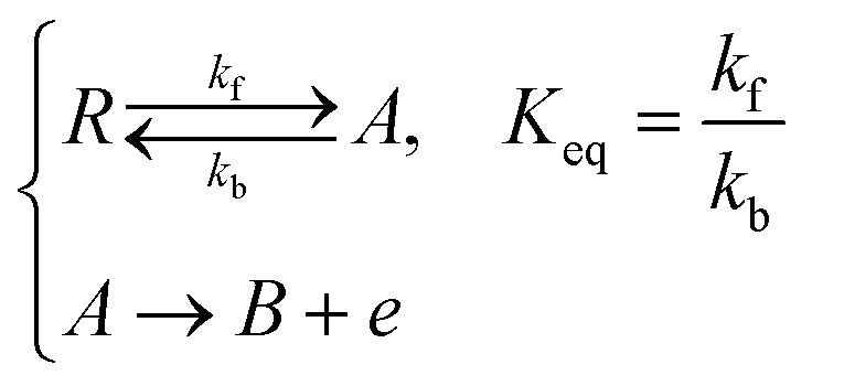
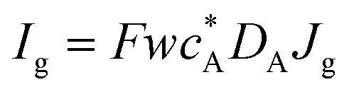
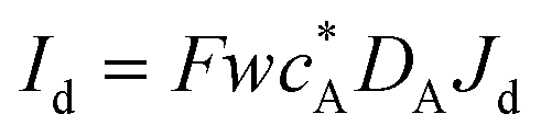
Three specific channel electrode problems are explored using PINNs in this paper. The first addresses the transport limited current arising from a simple one electron reaction, assumed to be an oxidation, at a channel microband electrode:where A and B are stable solution species flowing in the channel. The second problem is that of the double channel electrode working in generator-detector mode where the electrochemical reaction on the two electrodes are:| | 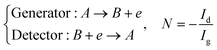 | (2) |
where Id and Ig are the currents of the detector and generator electrode respectively and N the collection efficiency of the double channel electrode where the case of both electrodes being of microband geometry is addressed. The third problem is that of preceding chemical reaction (a so-called CE reaction39) at a channel electrode where:| |  | (3) |
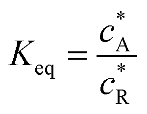
where A/B is the electrochemical redox couple and R is electrochemically inert. kf, kb and Keq are the forward reaction rate constant, reverse reaction rate constant and equilibrium constant of the preceding chemical reaction, respectively.
In all cases sufficient supporting electrolyte is presumed present so that the transport is exclusively via diffusion and forced convection. In this article, the simulation results are compared with previously reported analytical expression and/or experimental results where applicable.
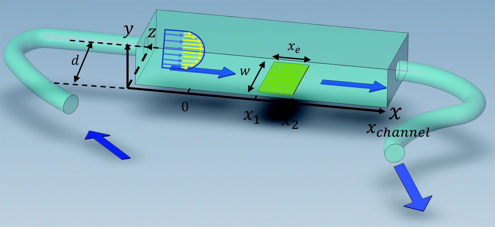
Solution flows through a cell such as shown in Fig. 1, which contains a rectangular electrode of length xe, width w. The distance xchannel represents the length of the flow cell which is simulated. As discussed below the distances, x1 and x2 (measured from the coordinate origin to the upstream edge or to the downstream edge of the electrode) define the position of the electrode within the PINN simulations. The distance x1 allows for axial diffusion upstream of the electrode whilst a distance xchannel − x2 is included in the simulation again to account for axial diffusion effects. The channel has a width of d and height of 2h.
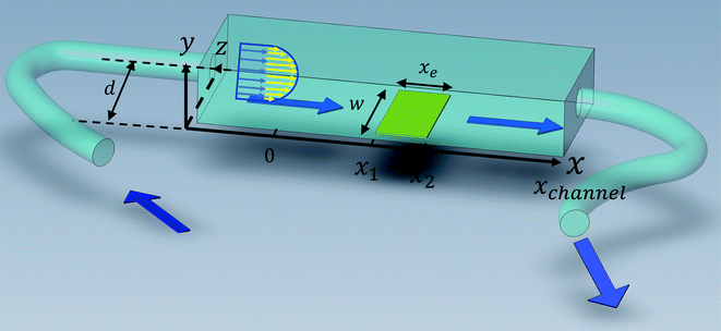 |
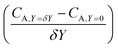
| | Fig. 1 A schematic illustration of single microband channel electrode. Parabolic velocity profile is allowed to developed before x = 0 and x = 0 is the start of simulation. The yellow arrows show the velocity profile of laminar flow. x1 and x2 are coordinates along x-axis measured to the upstream and downstream edge of channel and xchannel is the length of the flow cell. The height and width of flow cell is 2h and d along y and z axes respectively with x = 0 at the coordinate origin. The upstream and downstream lengths are denoted as xa and xb and the length and width of electrode are xe and w, respectively (see text). | |
The flow cell is usually designed that the flow pattern over the electrode is laminar and thus well-defined over the range of flow rates employed. Laminar or turbulent flow is usually characterized via the Reynold numbers where:
| |  | (4) |
and
v0 is the solution velocity at the center of channel and
ν is the kinematic viscosity of the solution. Re is usually experimentally kept below 2000 to avoid turbulent flow, which is more difficult to model. The steady-state flow is assumed to be fully developed at the upstream edge of the simulation which requires a lead-in length
xlead-in large enough to allow establishment of steady-state parabolic velocity profile (‘Poiseuille flow’) caused by the friction between the solution and the cells:
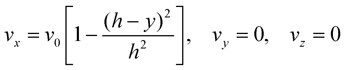
The fully developed laminar flow is described as:
| |  | (6) |
where
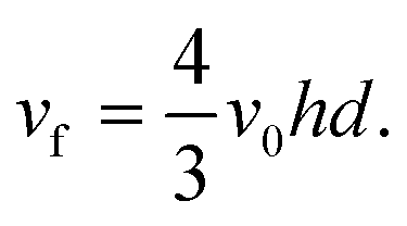
h is the half-height of the cell. The volume flow rate is:
| |  | (7) |
A similar parabolic profile is established across the diameter of tubular electrodes.21
3.1. Simulation of steady state limiting currents at single microband channel eectrodes
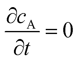
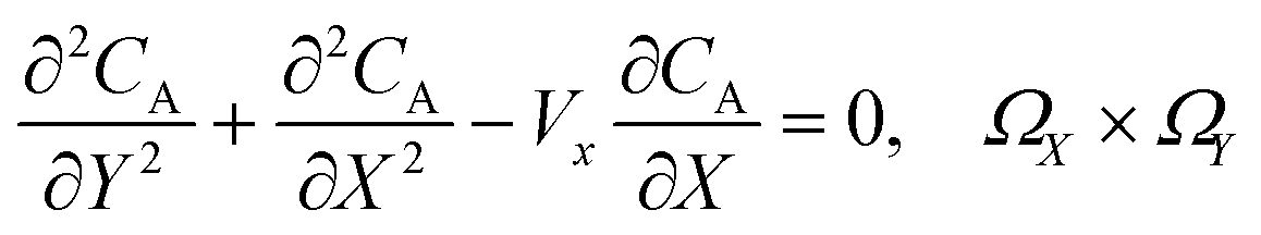
The mass transport equation for the channel electrode is:| |  | (8) |
where ∇2 is the Laplacian operator. Note that the flow rate in y and z directions is zero (vy = vz = 0) and at steady state  . Since the electrode width is usually much larger than the length, transverse diffusion in the z-direction can be neglected so reducing the simulation to a two-dimensional problem. Thus, the convective-diffusion mass transport at steady state simplifies to
| | 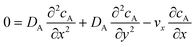 | (9) |
where DA is the diffusion coefficient of species A.
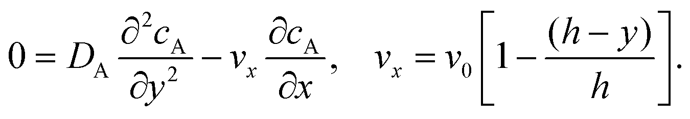
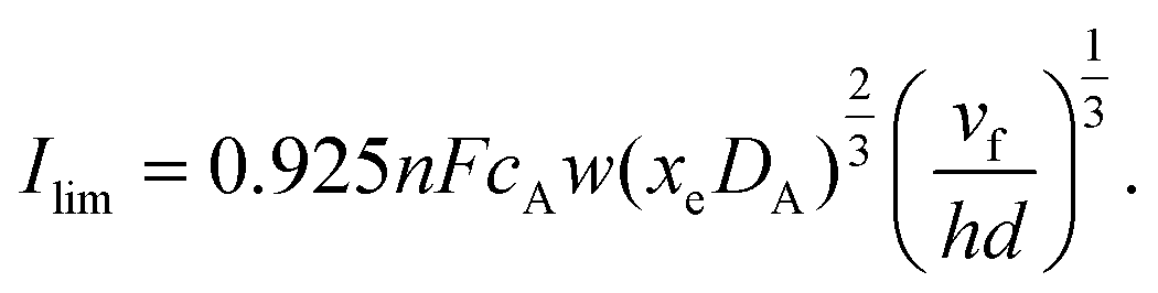
To facilitate an approximate analytical solution to the problem Levich10 further simplified by first neglecting axial diffusion which is a good approximation for macroelectrodes but not for microelectrodes40 and second by introducing the Lévêque approximation41 which linearizes the flow profile close to the electrode leading to:
| | 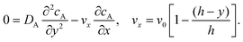 | (10) |
These simplifications allow derivation of the following approximate analytical expression for the transport limited current:
| | 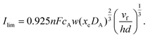 | (11) |
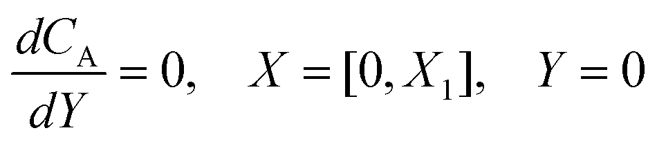
For the PINN simulation (see below for details) eqn (9) is solved subject to the following boundary conditions:
| | 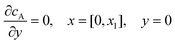 | (12.1) |
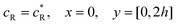
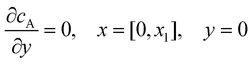
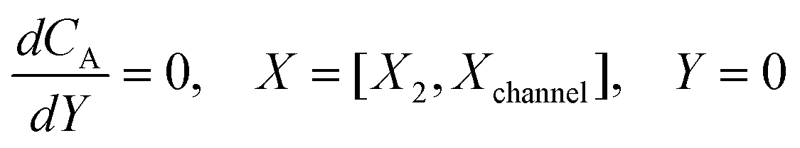
| | | cA = 0, x = [x1,x2], y = 0 | (12.2) |
| |  | (12.3) |
| |  | (12.4) |
| |  | (12.5) |
where

is the bulk concentration of
A at the inlet of channel where
B is not present.
Eqn (12.1, 12.3 and 12.5) represents the no-flux boundary conditions on the surface of insulating materials.
Eqn (12.2) enforces the zero concentration of
A on the surface of electrode due to the application of a high overpotential for the oxidation of A.
3.2. Simulation of a double microband channel electrode
Fig. 2 shows a schematic diagram of a double channel electrode where five distances are used to define the simulation space and the electrode geometry: x = 0 is the start of the simulation, x1 and x2 are the upstream and downstream coordinates of the generator electrode; x3 and x4 are the coordinates of the extremities of the detector electrode. xg = x2 − x1 and xd = x4 − x3 are the length of the generator and detector electrodes respectively. Note that the gap between the two electrodes, xb = x3 − x2, is a key parameter in controlling the collection efficiency.42,43
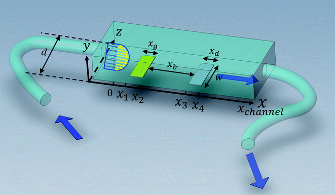 |
| | Fig. 2 A schematic illustration of double microband channel electrode. Parabolic velocity profile is allowed to developed before x = 0 and x = 0 is the start of simulation. The yellow arrows show the velocity profile of laminar flow. x1 and x2 are the upstream and downstream coordinates for generator electrode (golden) and x3 and x4 are upstream and downstream coordinates of detector electrode (metallic color). The height and width of flow cell is 2h and d along y and z axes respectively with x = 0 at the coordinate origin. The length of upstream, gap and downstream distances are denoted as xa, xb and xc respectively and the length of generator and detector electrode is xg and xd, respectively (see text). | |
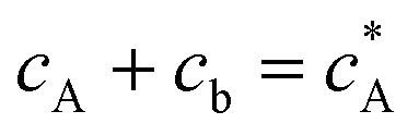
If species A and B in Fig. 2 are assumed to have identical diffusion coefficients at all points of space, then it can be shown that  . In this way the problem is reduced to just one species. Accordingly, the problem is formulated considering only the mass transport of A. The boundary conditions for double microband channel electrode specifies different concentration at the surface of the generator and detector electrodes.
| |  | (13.1) |
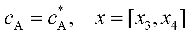
| | | cA = 0, x = [x1,x2], y = 0 | (13.2) |
| |  | (13.3) |
| |  | (13.4) |
| |  | (13.5) |
| |  | (13.6) |
| |  | (13.7) |
Eqn (13.1, 13.3, 13.5 and 13.7) correspond to no flux boundary conditions at the insulating wall of the channel electrode. The electrochemical reactions on the generator and detector electrodes are represented by eqn (13.2) and (13.4) respectively. Mass transport from upstream of channel electrode is represented by eqn (13.7).
3.3. Simulation of single channel electrode with CE reaction
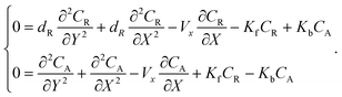
The mass transport equation for a channel electrode with coupled preceding chemical reaction at steady state is:| | 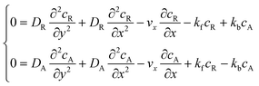 | (14) |
where DR is the diffusion coefficient for reactant R. Pre-equilibrium is assumed at x = 0 and in bulk solution for the preceding chemical reaction where  and
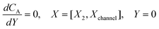
and  . The following boundary conditions describe the problem for calculating the transport limited current due to the reduction of A:
| |  | (15.1) |
| | | cA = 0, x = [x1,x2], y = 0 | (15.2) |
| |  | (15.3) |
| |  | (15.4) |
| |  | (15.5) |
The boundary conditions for the reactant, R, which is electrochemically inactive, are:
| |  | (16.1) |
| |  | (16.2) |
| |  | (16.3) |
3.4. Dimensionless parameters
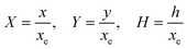
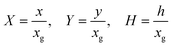
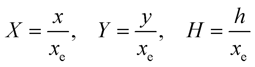
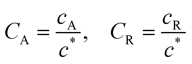
To solve the PDEs using PINN, dimensionless parameters (see Table 1) are pivotal to circumvent the expanding/diminishing gradient problem44 while increasing the generalizability of the models.12 By removing dependence on the electrode length, xe, diffusion coefficient, D, and bulk concentration, c*, the dimensionless results can be converted back to dimensional ones with any set of parameters. By definition, the dimensionless diffusion coefficient of A is always unity and not appear explicitly in the dimensionless mass transport equations. Without preceding chemical reaction, the dimensionless bulk concentration of species A is  ; with preceding chemical reaction and chemical equilibrium in the upstream solution,
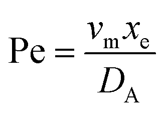
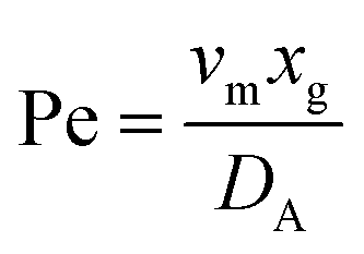
 . Using the length of electrode, xe, for a single channel electrode (and the length of generator electrode, xg, for double channel electrode) as a characteristic dimension and the Peclet number, Pe, reflects the relative influence of mass transport by convection and diffusion:
| |  | (17) |
where vm is the mean flow velocity given by  . The dimensionless form of mass transport equation, for single and double microband channel electrode is,
| | 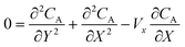 | (18) |
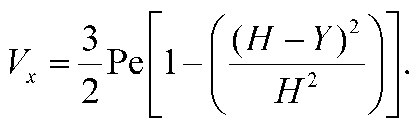
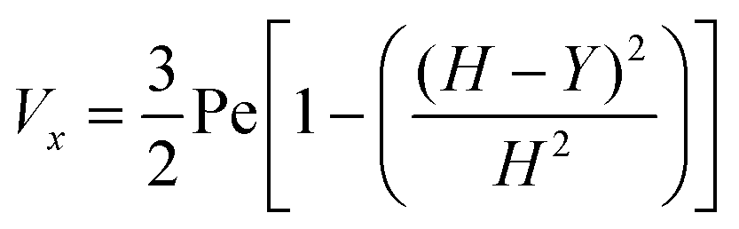
where (Table 1) the dimensionless flow rate, Vx, is:| |  | (19) |
Table 1 Table of conversions to dimensionless parameters. xe is the length of electrode for single microband channel electrode and xg is the length of generator electrode for double channel electrode. Dj stands for diffusion coefficient of any species j
| |
Single microband channel electrode |
Single microband channel electrode with CE reaction |
Double microband channel electrode |
| Spatial coordinate |
|

|
|
| Concentration |

|

|

|
| Diffusion coefficient |

|
| Peclet number |

|

|

|
| Velocity flow rate |

|
| First order chemical reaction |
N/A |

|
N/A |
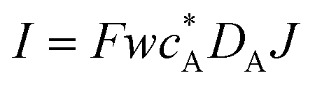
| Current |

|
I = Fwc*DAJ |

|

|
For channel electrode coupled with CE mechanics, the mass transport equation can be written as:
| |  | (20) |
3.5. PINN simulation
PINN simulation of the steady state mass transport with a single microband channel electrode requires prediction of concentration profile CA(X,Y) where X and Y are dimensionless coordinates. CA(X,Y) can be described as a combination of convective-diffusion equation and boundary conditions:| | 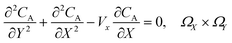 | (21.1) |
| |  | (21.2) |
| | | CA = 0, X = [X1,X2] | (21.3) |
| |  | (21.4) |
| |  | (21.6) |
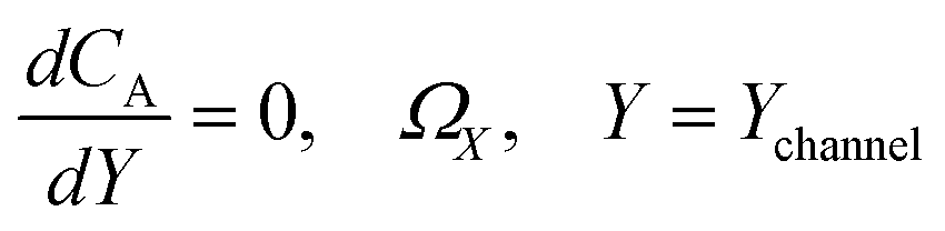
where ΩX ∈ [0,Xchannel], ΩY ∈ [0,Ychannel], and represent the two-dimensional spatial domain for simulation. Xchannel is the dimensionless simulation length in the X direction. While Xe is always equal to one by definition, X1 is set between 0.1 and 0.5 to allow diffusion upstream. Xchannel is thus between 1.2 and 2.0 to allow diffusion downstream. The faster the convection (high Pe), the less significant the contribution of axial diffusion and the smaller the Xchannel. Xchannel is chosen around 10 to 20 so that the boundary on the opposite side of electrode is less affected by the interfacial reaction(s). Eqn (21.1) represents the PDE to be solved using PINN; eqn (21.2) and (21.4) are the no-flux boundary conditions on the insulating surface. Eqn (21.6) describes the no-flux boundary condition at the outer boundary of simulation and is unperturbed by electrochemical reaction on the microband channel electrode. The electrochemical reaction on electrode surface is enforced by eqn (21.3) as the surface concentration of A is zero. Finally, eqn (21.5) enforces the boundary condition at the upstream of channel electrode, which should always be the bulk concentration of species A.
When neural networks are constrained by physical laws like the convective-diffusion equation above in eqn (21), they are said to be physical-informed. Unlike conventional supervised learning with neural network, which predicts C(X,Y) by feeding known concentrations corresponding to known spatial coordinates, PINN has only the knowledge of the physical equation and the boundary conditions. PINNs are trained by enforcing the physical laws with sets of collocation points, each set represents a physical constraint for PINN to satisfy. For example, to satisfy eqn (21.1),  collocation points
  are generated with a uniform random distribution on the ΩX × ΩY spatial domain to predict concentration,
  , while satisfying the physical constraint by minimizing the mean square error (MSE) of physical constraints:
| |  | (23) |
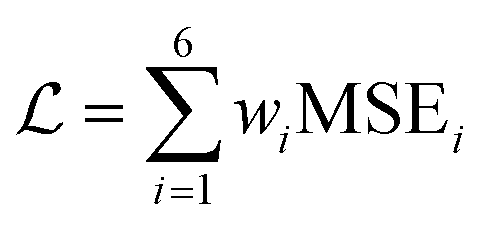
Calculation and optimization of PINN benefits from automatic differentiation (AD) commonly available in neural network frameworks, hence avoiding discretization and mesh setup. To satisfy the six equations of channel electrode, the overall loss of PINN is a linear combination of six MSE functions:
| |  | (23) |
where
wi is the weight of each MSE functions to accommodate errors which may have different magnitudes. During training, the overall loss is minimized by the Adam optimizer
45 (learning rate = 10
−3) and a hyperbolic tangent (tanh) is used as the activation function for its superior ability to approximate analytic functions.
46 The performance of the PINN depends on the number of collocation points,
47 and in this article

is set to 10
6 or 2 × 10
6 to satisfy both convergence and computer memory requirements. When the Peclet number, Pe > 10, curriculum learning (training stepwise from low Pe to high Pe) is used to assist convergence.
20
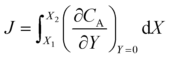
After training, a concentration profile at ΩX × ΩY is obtained. The flux on the surface of electrode is calculated as:
| | 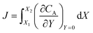 | (24) |
where

can be approximated as
.
Note that to predict the concentration of the two species in the CE reaction, two neural networks, each predicting one species, are integrated in the PINN. Details for implementation of double channel electrode and channel electrode with CE reaction is reported in the ESI.†
3.6. Simulation method
The simulation programs were written in Python and the neural networks were implemented using TensorFlow. The simulations were run using a Nvidia V100 GPU and 12 allocated CPU cores using the Advanced Research Computing (ARC) facility at the University of Oxford. The implementation is available at https://github.com/nmerovingian/PINN-Hydrodynamic-Voltammetry. The computational time is mentioned in the ESI.†
4. Results and discussion
In the following, first, PINN is applied to a single channel electrode and the predictions are compared with experimental results as a function of volume flow rate, vf. Second, a PINN prediction of the collection efficiency of a double channel electrode is made as a function of the electrode lengths and gap. The results are compared with limiting analytical expressions derived under the Lévêque approximation in the presence of axial diffusion. Third, PINN predictions of the steady state flux for a CE reaction at a single microband channel electrode are investigated.
4.1. Single microband channel electrode
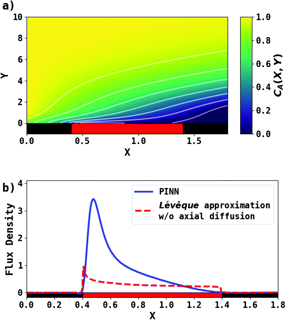
First, PINN simulation was conducted by setting Pe = 2.9. Fig. 3 presents the PINN prediction of steady state concentration profile and flux densities at the channel electrode. The concentration profiles show a progressive build-up of electrogenerated depletion in the direction of flow whilst this extends to a limited extent upstream of the electrode as a result of axial back-diffusion. Downstream of the electrode, the depletion spreads out into the bulk of the solution and gradually the local concentrations tend towards the upstream bulk value as convection replenishes the depletion. The flux density at the channel electrode, as shown in Fig. 3b, is not uniform. Note that in the limit of the Lévêque approximation and the neglect of axial diffusion, the flux scales as the inverse cube root of the distance from the upstream edge of the electrode which is approximately the case for the PINN results with the deviations attributed to the two approximations.
 |
| | Fig. 3 PINN prediction of transport-limited current at microband electrode when Pe = 2.9. (a) Concentration profile at steady state. (b) Flux density at steady state for the channel electrode using PINN without simplification (blue line); flux density predicted by PINN using Lévêque approximation and neglecting axial diffusion (red dashed-line). Red square represents the electrode and black squares are the insulating material. | |
To facilitate comparison with literature experimental results, the dimensionless PINN simulations were converted to dimensional values with the following parameters, 2h = 0.05 cm, w = 0.364 cm, d = 0.6 cm, D = 2.3 × 10⁻⁵ cm2 s−1, and  .36 Two electrode lengths, 4 μm and 11 μm were considered and the diffusion coefficients of all species were assumed to be 2.3 × 10⁻⁵ cm2 s−1. These diffusion coefficients correspond to ferrocene/ferrocenium redox couple in acetonitrile solution.36,48
To test the ‘convergence’ of the PINN, Fig. 4 illustrates the steady state flux predicted as a function of number of collocation points,  , for the case xe = 11 μm and vf = 0.004 cm3 s−1. It is seen that when
  , the steady state current converges to ca. 1.4 μA. For the simulations reported below, in Fig. 3 and Fig. 5, the value of
  was applied.
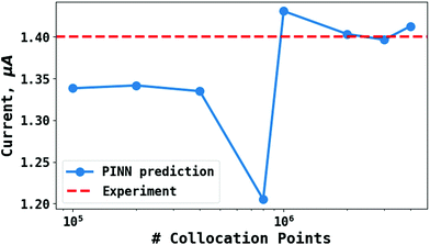 |
| | Fig. 4 PINN prediction of steady state current (blue line with marker) at 11 μm electrode and vf = 0.004 cm3 s−1 as a function of number of collocation points,  and compared with experimental results (red-dash line). and compared with experimental results (red-dash line). | |
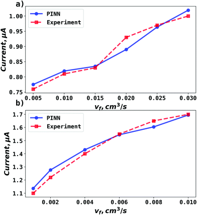 |
| | Fig. 5 Compare PINN prediction with experiment for oxidation of ferrocene at different electrode length. (a) Electrode length, xe = 4 μm. (b) Electrode length, xe = 11 μm. | |
PINN simulation of channel electrode was validated by comparing predictions for the ferrocene oxidation at the channel electrode with the experimental data36 which reports the effect of the volume flow rate on the limiting current for the two channel electrodes of different lengths given above: from 0.005 to 0.03 cm3 s−1 for 4 μm electrode (Pe = 2.90 to 17.37) and 0.001 to 0.01 cm3 s−1 (Pe = 1.59 to 15.94) for 11 μm electrode. Fig. 5 presents the PINN predicted steady state current and experimental current as a function of volume flow rate, vf. Good agreement with experimental results is observed as the maximum difference from experimental currents is less than 0.05 μA, suggesting that PINN can quantitatively predict the steady state current for microband channel electrodes under conditions where both diffusions, axial and normal, as well as convection contribute to the mass transport.
PINN simulations were attempted for simplified models in which the axial diffusion was turned off and/or the Lévêque approximation made in place of eqn (10). In Fig. 3b, the red-dashed line illustrates the flux density with Lévêque approximation and neglecting axial diffusion. Compared with the solid blue line representing PINN prediction without approximations, the red-dashed line shows a lower flux density and a sharper peak in the flux at the upstream edge of electrode, showing the greater relative contribution of convection when axial diffusion is assumed to be absent. It is interesting to note that the PINN solution was more easily successful with the physically realistic model whereas it was quantitatively challenged by the two approximations previous used to enable analytical mathematical approaches.
4.2. Double microband channel electrode
We consider the case of a double microband channel electrode which employs a generator-detector setup,49 in which a downstream detector electrode reduces the electro-generated product, B, from the electro-oxidation of A at an upstream generator electrode. The ratio of the detector electrode current relative to the generator electrode current is termed the collection efficiency, N, which for a stable species undergoing transport is controlled by the geometry of the double channel electrode and the flow rate.
To explore these parameters, we made PINN prediction while keeping the length of both the generator and the detector electrode identical, with the dimensionless gap Xb between the electrodes, varied from  to 1 and Pe fixed at 100. The upstream simulation space is enforced by setting
  and the downstream space by fixing
  . The simulation distance in Y direction is Ychannel = 2.5Xchannel. The number of collocation points, for the simulations shown in Fig. 6 and 7 was
  .
.
 |
| | Fig. 6 PINN prediction of double channel electrode at steady state by varying Xb from  to 1 with a step size of to 1 with a step size of  while the length of generator and detector electrode are equal. (left) Concentration profile at steady state. Generator electrode, detector electrode and insulating material are represented with red, green and black boxes. (right) Flux density at each electrode. Red line and blue line are for generator and detector electrode respectively. while the length of generator and detector electrode are equal. (left) Concentration profile at steady state. Generator electrode, detector electrode and insulating material are represented with red, green and black boxes. (right) Flux density at each electrode. Red line and blue line are for generator and detector electrode respectively. | |
 |
| | Fig. 7 Compare PINN prediction of collection efficiency (N) with Matsuda/Braun equation as a function of dimensionless gap distance Xb. | |
The concentration profiles and flux densities predicted by the PINN are shown in Fig. 6. The concentration profiles show a plume of electrogenerated material flowing downstream and being partially but not completely consumed at the detector electrode. The electrogenerated material extends upstream of the generator electrode where it is carried by axial diffusion against the flow.
The plots of the flux density on the generator electrode show two maxima. The upstream peak resembles that observed above for a single channel electrode and again reflects the high flux delivered convectively and diffusively in this region. The second (downstream peak) is attributed to axial back diffusion against the flow leading to upstream transport of some A following regeneration from B at the detector electrode (eqn (2)). With increasing gap distance, the flux density in the second peak in the generator flux decrease relatively to the first peak because the ‘positive feedback’ from the detector electrode decreases. In addition, note that a longer gap length facilitates the diffusion of electrochemically generated B away from surface of electrode, leading to reduced flux density at the detector electrode.
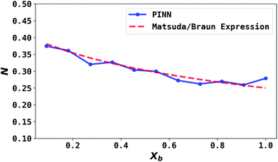
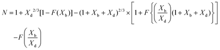
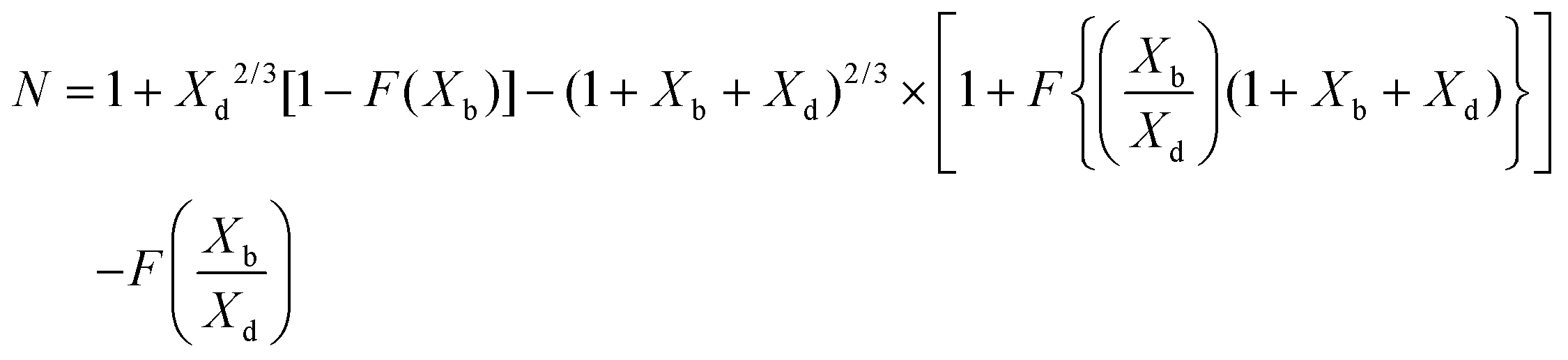
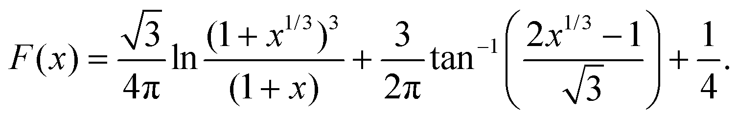
To validate the PINN prediction, the predicted collection efficiency was compared with analytical expressions. Matsuda and Braun43,50,51 have developed approximate analytical expressions for the collection efficiency of a double channel electrode as:
| |  | (25) |
where
Xb and
Xd are the dimensionless gap and detector electrode length respectively. The function
F is tabulated by Albery and Bruckenstein
42 as:
| |  | (26) |
The collection efficiency predicted by PINN is compared with the predictions of the Matsuda/Braun expression in Fig. 7 and a good agreement is observed between the two, suggesting that PINN can quantitatively simulate the mass transport of a double microband electrode and generate a good estimate of the collection efficiency.
4.3. Channel electrode with CE reaction
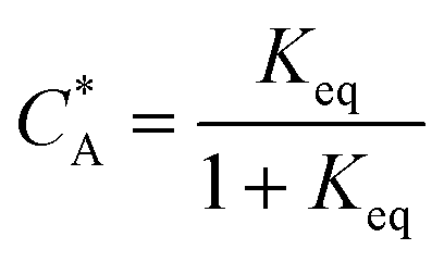
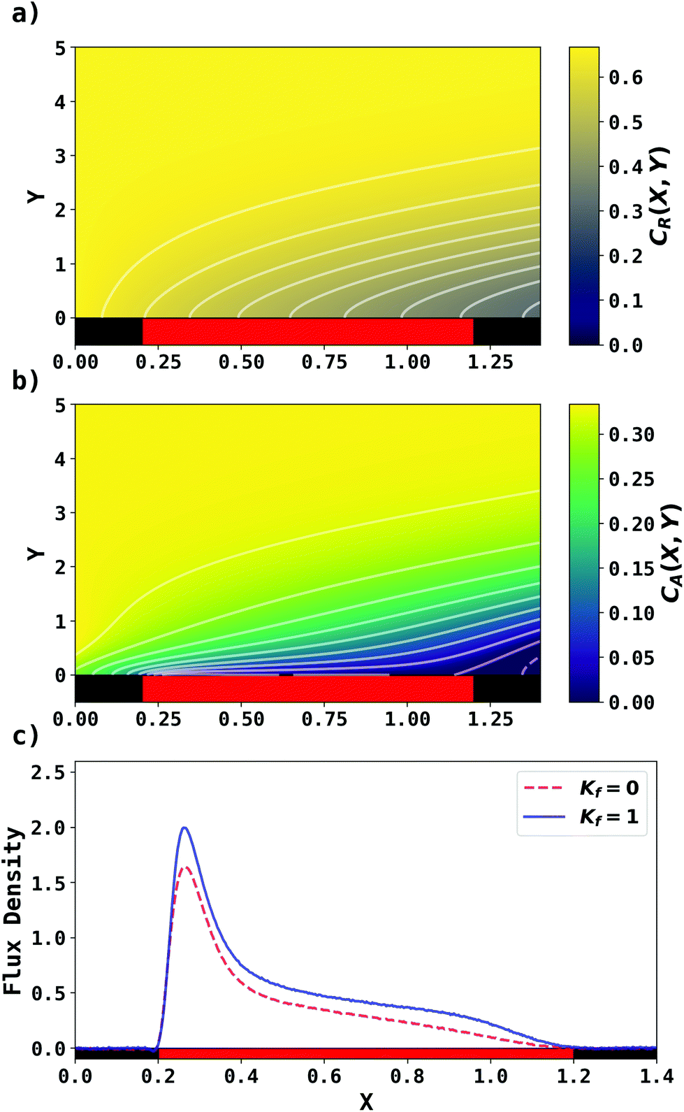
As a third paradigm case, PINN simulations of a microband channel electrode assuming xe = 11 μm with CE reaction are performed with increasing dimensionless forward reaction rate constants, from Kf = 0 to Kf = 100 while fixing Keq = 0.5. Hence, the dimensionless concentrations of R and A in bulk equilibrated solution, prior to entering the flow cell and upstream of the electrode are  and
and  respectively and
  . Two flow rates are considered: Pe = 1.59 and 6.38, and the corresponding volume flow rates are vf = 0.001 cm3 s−1 and 0.004 cm3 s−1. The number of collocation points are set to
  . Fig. 8 shows the concentration profiles of A and R and the flux density of a PINN simulation when Kf = 1 and Pe = 1.59 Fig. 8a illustrates the depletion of R near the surface of electrode, to generate A, as the subsequent removal of A pushes the chemical equilibrium towards product; Fig. 8b presents the concentration profile of A, showing depletion of A along the flow direction and mass transport upstream due to axial back-diffusion. The pattern of concentration profile is like Fig. 3a, but the concentration gradients differ and result in different flux densities. From Fig. 8c, the flux density when Kf = 1 is higher than Kf = 0, reflecting the extra current contribution from the preceding chemical reaction generating extra A for consumption at the electrode.
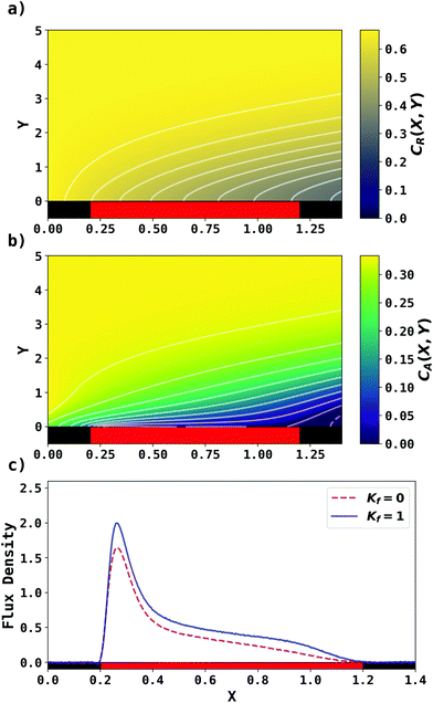 |
| | Fig. 8 PINN prediction of channel electrode coupled with CE reaction, when Kf = 1, Keq = 0.5 and Pe = 1.59. (a and b) Concentration profile of R and A respectively. (c) Flux density of electrochemical reaction of A when Kf = 0 and Kf = 1. | |
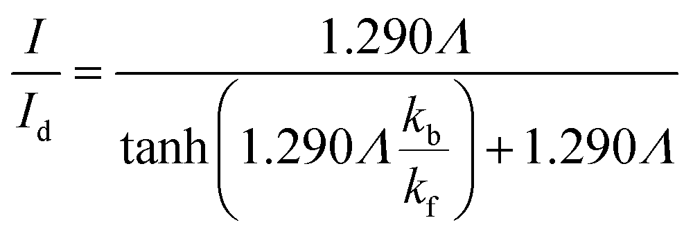
Matsuda et al.52 developed an approximate analytical expression relating the diffusion-controlled current with the kinetic current by neglecting axial diffusion:
| |  | (27) |
where
Id is the diffusion-limited current assuming that the bulk dimensionless concentration

and ∧ is a dimensionless parameter reflecting kinetic, thermodynamic and mass transport parameters derived assuming the diffusion coefficients of all species are equal to that of A:
| | 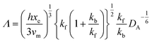 | (28) |
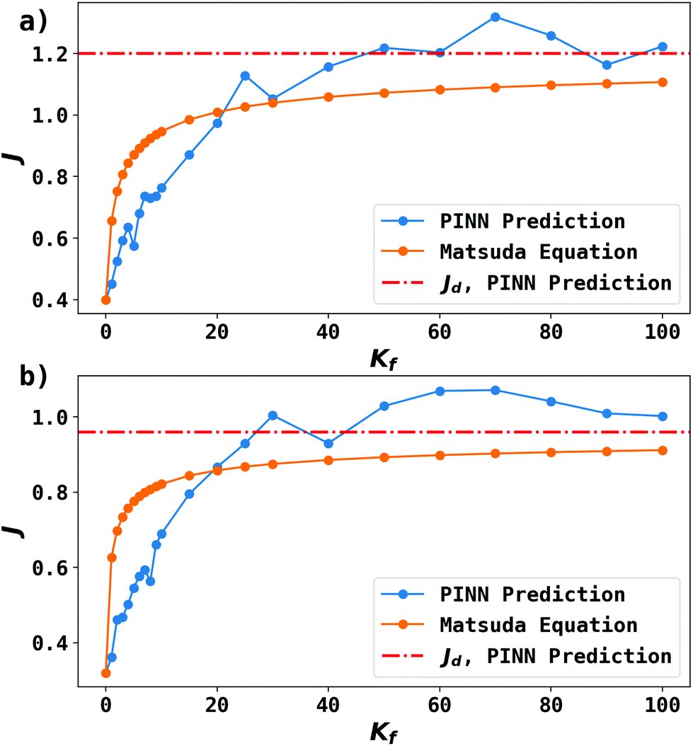
Fig. 9 shows the PINN prediction of transport limited currents as a function of Kf at Keq = 0.5 and two different Pe: (a) 6.38, (b) 1.59. The PINN predictions (blue line with marker) were benchmarked with the Matsuda equation (orange line with marker) and Fig. 9 suggests that the two lines approach the diffusion limited current (red dash-dot line) with increasing Kf. As expected increasingly fast homogeneous kinetics leads to increased currents as more A is made available for reaction on the voltammetric timescale. However, the PINN prediction suggests that in comparison with the Matsuda equation, faster homogeneous kinetics are generally required to access the same currents in the kinetically controlled regime consistent with the fact that the electrode modelled is of microelectrode dimensions and so experiences a shorter voltammetric timescale than the Matsuda equation designed for macroelectrodes. On the other hand, the increased rate of mass transport leads to the establishment of the full diffusion-controlled limit for lower values of Kf. The mathematical derivations of eqn (27 and 28) are at the limits of analytical theory and require the adoption of severe approximations. It is evident that PINNs have the potential to make predictions via physically more realistic models.
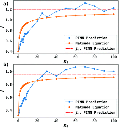 |
| | Fig. 9 PINN prediction of kinetic flux (orange line with marker) as a function of dimensionless forward reaction rate constant at fixed Keq and comparison with flux predicting by Matsuda equation (blue line with marker). Red dash-dot line represents the mass transport limiting current when  . (a) Keq = 0.5, Pe = 6.38, (b) Keq = 0.5, Pe = 1.59. . (a) Keq = 0.5, Pe = 6.38, (b) Keq = 0.5, Pe = 1.59. | |
5. Conclusions
In summary, we have implemented PINNs to solve three problems in hydrodynamic voltammetry: transport limited currents at single microband channel electrodes, the collection efficiency of a double microband channel electrode and the kinetically controlled currents expected at a channel electrode for a CE reaction. The resulting steady-state currents were compared with experiments or analytical expression where available, proving that PINNs is a rapid and simple to implement alternative to FD and FE simulations for solving electroanalytical convective-diffusion problems including those with coupled homogeneous chemical kinetics. In the latter case we facilitated PINN solution for the prediction of the concentration of two species via the cooperation of two embedded neural networks in the PINN. We have also demonstrated that PINNs can be applied to convection-diffusion problems with fast mass transport (high Pe number), using curriculum learning to accelerate convergence. Together with our previous paper on diffusion only voltammetry,53 the work on hydrodynamic voltammetry establishes the basis of PINN simulation for the application of PINNs in electrochemistry and electro-analytical chemistry, being an easier and/or cheaper alternative to finite element or finite difference method.
Conflicts of interest
There are no conflicts to declare.
Acknowledgements
Haotian Chen and Richard Compton would like to acknowledge the use of the University of Oxford Advanced Research Computing (ARC) facility in carrying out this work (https://dx.doi.org/10.5281/zenodo.22558). Haotian Chen thanks Lady Margaret Hall for a 2020/2021 postgraduate scholarship award.
References
-
Q. Chang, China lifts 770 million rural people out of poverty: white paper, https://en.people.cn/n3/2021/0414/c90000-9838854.html, (accessed Feburary 18, 2020).
-
Scientific method
, https://www.britannica.com/science/scientific-method, (accessed Feburary 17, 2022).
- J. A. V. Butler, Trans. Faraday Soc., 1924, 19, 729–733 RSC.
- T. Erdey-Grúz and M. Volmer, Z. Phys. Chem., 1930, 150, 203–213 CrossRef.
- R. A. Marcus, J. Chem. Phys., 1956, 24, 966–978 CrossRef CAS.
- R. A. Marcus, J. Chem. Phys., 1957, 26, 867–871 CrossRef CAS.
- N. S. Hush, J. Chem. Phys., 1958, 28, 962–972 CrossRef CAS.
- A. Fick, Ann. Phys., 1855, 170, 59–86 CrossRef.
- A. Fick, London, Edinburgh Dublin Philos. Mag. J. Sci., 1855, 10, 30–39 CrossRef.
-
V. G. Levich, Physicochemical hydrodynamics, 1962 Search PubMed.
- A. Frumkin, Z. Phys., 1926, 35, 792–802 CrossRef CAS.
-
R. G. Compton, E. Laborda, E. Kaetelhoen and K. R. Ward, Understanding voltammetry: simulation of electrode processes, World Scientific London, 2nd edn, 2020 Search PubMed.
-
D. Britz and J. Strutwolf, Digital simulation in electrochemistry, Springer, 2005 Search PubMed.
- C. Rao, H. Sun and Y. Liu, Theor. Appl. Mech. Lett., 2020, 10, 207–212 CrossRef.
- X.-D. Bai and W. Zhang, Comput. Fluids, 2022, 235, 105266 CrossRef.
- Y. Huang, Y. Tang, H. Zhuang, J. VanZwieten and L. Cherubin, Front. Artif. Intell., 2021, 4, 780271 CrossRef PubMed.
- Y. Bai, T. Chaolu and S. Bilige, Nonlinear Dyn., 2022, 107, 3655–3667 CrossRef.
- M. Aykol, C. B. Gopal, A. Anapolsky, P. K. Herring, B. van Vlijmen, M. D. Berliner, M. Z. Bazant, R. D. Braatz, W. C. Chueh and B. D. Storey, J. Electrochem. Soc., 2021, 168, 030525 CrossRef CAS.
- Y. A. Yucesan and F. A. Viana, Int. J. Progn. Health Manag., 2020, 11 Search PubMed , http://papers.phmsociety.org/index.php/ijphm/article/view/2594.
- A. Krishnapriyan, A. Gholami, S. Zhe, R. Kirby and M. W. Mahoney, Adv. Neural Inf. Process. Syst., 2021, 34, 26548–26560 Search PubMed.
- R. G. Compton and P. R. Unwin, J. Electroanal. Chem. Interfacial Electrochem., 1986, 205, 1–20 CrossRef CAS.
- J. A. Cooper and R. G. Compton, Electroanalysis, 1998, 10, 141–155 CrossRef CAS.
- J. A. Alden, M. A. Feldman, E. Hill, F. Prieto, M. Oyama, B. A. Coles, R. G. Compton, P. J. Dobson and P. A. Leigh, Anal. Chem., 1998, 70, 1707–1720 CrossRef CAS PubMed.
- J. Alden and R. Compton, Anal. Chem., 2000, 72(5), 198 A–203 A CrossRef CAS PubMed.
- B. A. Coles and R. G. Compton, J. Electroanal. Chem. Interfacial Electrochem., 1983, 144, 87–98 CrossRef CAS.
-
J. Ruzicka and E. H. Hansen, Flow injection analysis, John Wiley & Sons, 1988, vol. 104 Search PubMed.
- J. Ruzicka, Anal. Chem., 1983, 55, 1040A–1053A CAS.
- D. A. Roston, R. E. Shoup and P. T. Kissinger, Anal. Chem., 1982, 54, 1417A–1434A CAS.
- D. A. Roston and P. T. Kissinger, Anal. Chem., 1982, 54, 429–434 CrossRef CAS.
- C. Renault, M. J. Anderson and R. M. Crooks, J. Am. Chem. Soc., 2014, 136, 4616–4623 CrossRef CAS PubMed.
- H. Wang, E. Rus and H. D. Abruña, Anal. Chem., 2010, 82, 4319–4324 CrossRef CAS PubMed.
- J. Booth, R. G. Compton, J. A. Cooper, R. A. Dryfe, A. C. Fisher, C. L. Davies and M. K. Walters, J. Phys. Chem., 1995, 99, 10942–10947 CrossRef CAS.
- A. J. Wain, R. G. Compton, R. Le Roux, S. Matthews, K. Yunus and A. C. Fisher, J. Phys. Chem. B, 2006, 110, 26040–26044 CrossRef CAS PubMed.
- S. Liu, Y. Gu, R. B. Le Roux, S. M. Matthews, D. Bratton, K. Yunus, A. C. Fisher and W. T. Huck, Lab Chip, 2008, 8, 1937–1942 RSC.
- S. S. Hill, R. A. W. Dryfe, E. P. L. Roberts, A. C. Fisher and K. Yunus, Anal. Chem., 2003, 75, 486–493 CrossRef CAS PubMed.
- R. G. Compton, A. C. Fisher, R. G. Wellington, P. J. Dobson and P. A. Leigh, J. Phys. Chem., 1993, 97, 10410–10415 CrossRef CAS.
- C. Amatore, N. Da Mota, C. Lemmer, C. Pebay, C. Sella and L. Thouin, Anal. Chem., 2008, 80, 9483–9490 CrossRef CAS PubMed.
- T. Holm, J. A. Diaz Real and W. Mérida, J. Electroanal. Chem., 2019, 842, 115–126 CrossRef CAS.
- A. Testa and W. Reinmuth, Anal. Chem., 1961, 33, 1320–1324 CrossRef CAS.
-
R. G. Compton and C. E. Banks, Understanding voltammetry, World Scientific, London, 3rd edn, 2018 Search PubMed.
-
A. Lévêque, Les lois de la transmission de chaleur par convection, Dunod, 1928 Search PubMed.
- W. J. Albery and S. Bruckenstein, Trans. Faraday Soc., 1966, 62, 1920–1931 RSC.
- H. Matsuda, J. Electroanal. Chem. Interfacial Electrochem., 1968, 16, 153–164 CAS.
-
F. M. Rohrhofer, S. Posch and B. C. Geiger, arXiv preprint arXiv:2105.00862, 2021.
-
D. P. Kingma and J. Ba, arXiv preprint arXiv:1412.6980, 2014.
- T. De Ryck, S. Lanthaler and S. Mishra, Neural Netw., 2021, 143, 732–750 CrossRef PubMed.
-
R. Leiteritz and D. Pflüger, arXiv preprint arXiv:2112.05620, 2021.
- Y. Wang, E. I. Rogers and R. G. Compton, J. Electroanal. Chem., 2010, 648, 15–19 CrossRef CAS.
- E. O. Barnes, G. E. Lewis, S. E. Dale, F. Marken and R. G. Compton, Analyst, 2012, 137, 1068–1081 RSC.
- H. Gerischer, I. Mattes and R. Braun, J. Electroanal. Chem., 1965, 10, 553–567 CAS.
- R. Braun, J. Electroanal. Chem. Interfacial Electrochem., 1968, 19, 23–35 CrossRef CAS.
- K. Tokuda, K. Aoki and H. Matsuda, J. Electroanal. Chem. Interfacial Electrochem., 1977, 80, 211–222 CrossRef CAS.
- H. Chen, E. Kätelhön and R. G. Compton, J. Phys. Chem. Lett., 2022, 13, 536–543 CrossRef CAS PubMed.
|
| This journal is © The Royal Society of Chemistry 2022 |
Click here to see how this site uses Cookies. View our privacy policy here. 
 Open Access Article
 This Open Access Article is licensed under a
  a,
Enno
Kätelhön
b and
Richard G.
Compton
a,
Enno
Kätelhön
b and
Richard G.
Compton


 . Since the electrode width is usually much larger than the length, transverse diffusion in the z-direction can be neglected so reducing the simulation to a two-dimensional problem. Thus, the convective-diffusion mass transport at steady state simplifies to
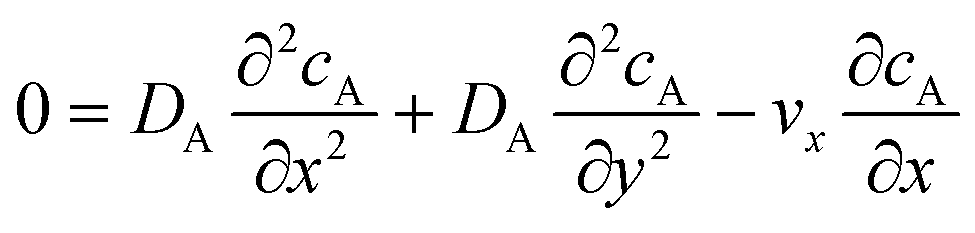


 is the bulk concentration of A at the inlet of channel where B is not present. Eqn (12.1, 12.3 and 12.5) represents the no-flux boundary conditions on the surface of insulating materials. Eqn (12.2) enforces the zero concentration of A on the surface of electrode due to the application of a high overpotential for the oxidation of A.

 . In this way the problem is reduced to just one species. Accordingly, the problem is formulated considering only the mass transport of A. The boundary conditions for double microband channel electrode specifies different concentration at the surface of the generator and detector electrodes.


 and
and 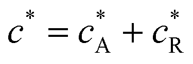 . The following boundary conditions describe the problem for calculating the transport limited current due to the reduction of A:


 ; with preceding chemical reaction and chemical equilibrium in the upstream solution,
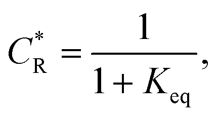
 . Using the length of electrode, xe, for a single channel electrode (and the length of generator electrode, xg, for double channel electrode) as a characteristic dimension and the Peclet number, Pe, reflects the relative influence of mass transport by convection and diffusion:
 . The dimensionless form of mass transport equation, for single and double microband channel electrode is,
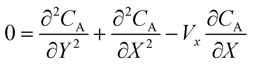


 collocation points
  are generated with a uniform random distribution on the ΩX × ΩY spatial domain to predict concentration,
  , while satisfying the physical constraint by minimizing the mean square error (MSE) of physical constraints:
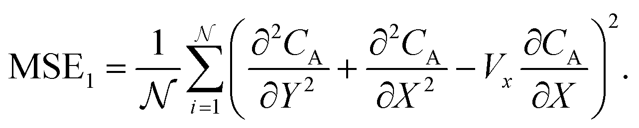
 is set to 106 or 2 × 10⁶ to satisfy both convergence and computer memory requirements. When the Peclet number, Pe > 10, curriculum learning (training stepwise from low Pe to high Pe) is used to assist convergence.20
 can be approximated as
  .
.
 .36 Two electrode lengths, 4 μm and 11 μm were considered and the diffusion coefficients of all species were assumed to be 2.3 × 10⁻⁵ cm2 s−1. These diffusion coefficients correspond to ferrocene/ferrocenium redox couple in acetonitrile solution.36,48
 , for the case xe = 11 μm and vf = 0.004 cm3 s−1. It is seen that when
  , the steady state current converges to ca. 1.4 μA. For the simulations reported below, in Fig. 3 and Fig. 5, the value of
  was applied.
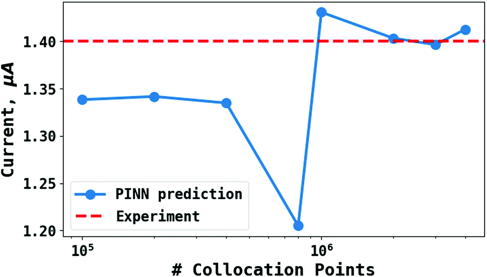
 and compared with experimental results (red-dash line).
 to 1 and Pe fixed at 100. The upstream simulation space is enforced by setting
  and the downstream space by fixing
  . The simulation distance in Y direction is Ychannel = 2.5Xchannel. The number of collocation points, for the simulations shown in Fig. 6 and 7 was
  .
.
 to 1 with a step size of
  while the length of generator and detector electrode are equal. (left) Concentration profile at steady state. Generator electrode, detector electrode and insulating material are represented with red, green and black boxes. (right) Flux density at each electrode. Red line and blue line are for generator and detector electrode respectively.
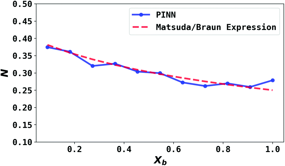
 and
and  respectively and
  . Two flow rates are considered: Pe = 1.59 and 6.38, and the corresponding volume flow rates are vf = 0.001 cm3 s−1 and 0.004 cm3 s−1. The number of collocation points are set to
  . Fig. 8 shows the concentration profiles of A and R and the flux density of a PINN simulation when Kf = 1 and Pe = 1.59 Fig. 8a illustrates the depletion of R near the surface of electrode, to generate A, as the subsequent removal of A pushes the chemical equilibrium towards product; Fig. 8b presents the concentration profile of A, showing depletion of A along the flow direction and mass transport upstream due to axial back-diffusion. The pattern of concentration profile is like Fig. 3a, but the concentration gradients differ and result in different flux densities. From Fig. 8c, the flux density when Kf = 1 is higher than Kf = 0, reflecting the extra current contribution from the preceding chemical reaction generating extra A for consumption at the electrode.
 and ∧ is a dimensionless parameter reflecting kinetic, thermodynamic and mass transport parameters derived assuming the diffusion coefficients of all species are equal to that of A:
 . (a) Keq = 0.5, Pe = 6.38, (b) Keq = 0.5, Pe = 1.59.