
Electroanalytical profiling of cocaine samples by means of an electropolymerized molecularly imprinted polymer using benzocaine as the template molecule†
Renata A.
Grothe
 a,
Alnilan
Lobato
a,
Bassim
Mounssef
Jr.
a,
Nikola
Tasić
a,
Ataualpa A. C.
Braga
a,
Adriano O.
Maldaner
b,
Leigh
Aldous
c,
Thiago R. L. C.
Paixão
*a and
Luís Moreira
Gonçalves
*a
a,
Alnilan
Lobato
a,
Bassim
Mounssef
Jr.
a,
Nikola
Tasić
a,
Ataualpa A. C.
Braga
a,
Adriano O.
Maldaner
b,
Leigh
Aldous
c,
Thiago R. L. C.
Paixão
*a and
Luís Moreira
Gonçalves
*a
aDepartamento de Química Fundamental, Instituto de Química, Universidade de São Paulo (USP), Avenida Prof. Lineu Prestes, 748, Cidade Universitária, São Paulo – SP, 05508-000, Brazil. E-mail: trlcp@iq.usp.br
bInstituto Nacional de Criminalística, Polícia Federal Brasileira (PFB), Q7, L23, Asa Sul, Brasília – DF, 70610-200, Brazil. E-mail: lmgoncalves@iq.usp.br
cDepartment of Chemistry, King's College of London, Britannia House, 7 Trinity Street, London, SE1 1DB, UK
First published on 12th January 2021
Abstract
The analysis of ‘cutting’ or additive agents in cocaine, like benzocaine (BZC), allows police analysts to identify each component of the sample, thus obtaining information like the drugs’ provenience. This kind of drug profiling is of great value in tackling drug trafficking. Electropolymerized molecularly imprinted polymers (e-MIPs) on portable screen-printed carbon electrodes (SPCEs) were developed in this study for BZC determination. The MIPs’ electropolymerization was performed on a carbon surface using the anaesthetic BZC as the template molecule and 3-amino-4-hydroxybenzoic acid (3,4-AHBA) as the functional monomer. The build-up of this biomimetic sensor was carefully characterized by cyclic voltammetry (CV) and optimized. Cyclic voltammetric investigation demonstrated that BZC oxidation had a complex and pH-dependent mechanism, but at pH 7.4 a single, well-defined oxidation feature was observed. The BZC-MIP interactions were studied by computer-aided theoretical modeling by means of density functional theory (DFT) calculations. The electroanalytical methodology was effectively applied to artificial urine samples; BZC molecular recognition was achieved with a low limit of detection (LOD) of 2.9 nmol L−1 employing square-wave voltammetry (SWV). The e-MIPs were then used to ‘fingerprint’ genuine cocaine samples, assisted by principal component analysis (PCA), at the central forensic laboratory of the Brazilian Federal Police (BFP) with a portable potentiostat. This electroanalysis provided proof-of-concept that the drugs could be voltammetrically ‘fingerprinted’ using e-MIPs supported by chemometric analysis.
1. Introduction
The analysis of ‘contaminants’ in drugs allows police experts to establish a profile of seized products, creating a sort of ‘fingerprint’ of each sample. This is of great importance for law enforcement agencies, as it makes it possible to compare and confirm that different samples have the same origin, allowing experts to better tackle continental and world trafficking.1 Significantly, some of the adulterants used to ‘volume boost’ narcotics are even more dangerous than the intended active ingredient.2 Benzocaine (BZC, ethyl 4-aminobenzoate) is a local anaesthetic that acts momentarily upon application, ceasing the stimulation and conductivity of nerve receptors, thus causing a loss of perception and relieving local pain stimuli.3,4 More specifically, BZC blocks sodium channels and, consequently, reduces an action potential in cell membranes to cause this lack of sensitivity.5 BZC is one of the most widely accepted short-duration topical anaesthetic drugs, is commonly used in dentistry, and applied through mucous membranes.6 It is also used as a topical pain reliever, and active ingredient in sore throat medicines7 and in ear wax removing remedies.8 However, in recent years BZC has been increasingly used as an adulterant during volume-boosting of street-cocaine samples,9,10 given its widespread availability as a white powder, and its cocaine-like numbing of gums. It is also finding increasing use as a functional additive in “legal highs” (i.e. commercial products for human use with confirmed psychoactive effects), such as the so-called ‘plant feeders’ or ‘bath salts’.11,12,100A literature survey demonstrated extremely few studies have reported on the electroanalysis of BZC (Table 1),3,13–15 in various types of samples. There is only one report on molecularly imprinted polymers (MIPs) for BZC quantification: Sun et al. developed molecularly imprinted microspheres via aqueous-suspension polymerization with methacrylic acid as the functional monomer. The microspheres were then used in a molecularly imprinted solid-phase extraction system to extract BZC in human serum and fish tissue, prior to BZC analysis and quantification by high-performance liquid chromatography with UV spectrophotometric detection (HPLC-UV).16 This means that, to the best of the authors‘ knowledge, so far electropolymerized MIPs (e-MIPs) have not been developed for BZC detection and quantification.
| Electroanalytical technique | Electrode | LOD/μmol L−1 | LOQ/μmol L−1 | Matrix | Ref. |
|---|---|---|---|---|---|
| ABS – acetate buffer solution; BDDE – boron-doped diamond electrode; BRB – Britton–Robinson buffer; cap-b-MWCNT-BPPGE – capsaicin modified bamboo-like multiwalled carbon nanotube modified basal plane pyrolytic graphite electrode; CPE – carbon paste electrode; CV – cyclic voltammetry; DME – dropping mercury electrode; DPAdSV – differential pulse adsorptive stripping voltammetry; DPV – differential pulse voltammetry; Nf – nafion; p-CMCPE: p-chloranil modified carbon paste electrode; PBS – phosphate buffer solution; PT – polythiophene; PtE – platinum electrode; TiO2-GO/CPE – titanium dioxide – graphene oxide/carbon paste electrode. | |||||
| SWV | GCE-MIP | 0.0029 | 0.0098 | Artificial urine | This work |
| SPCE-MIP | 0.059 | 0.20 | PBS, pH 7.4 | ||
| Bromatometry | Helical PtE | — | — | HCl, pH 1 | 91 |
| SWV | BDDE | — | — | BRB, pH 1.6 | 84 |
| Bromatometry | PtE | — | — | H2SO4, pH 1 | 92 |
| DPAdSV | Nafion-GCE | 0.0024 | 0.0080 | BRB, pH 2 | 61 |
| SWV | Cap-b-MWCNT-BPPGE | 2.5 | — | BRB, pH 1 | 93 |
| p-CMCPE | 4.3 | ||||
| DPV | Miniaturized BDDE | 0.08 | — | BRB, pH 4 | 13 |
| SWV | 0.1 | ||||
| Amperometry | CPE | 0.19 | — | BRB, pH 4 | 94 |
| SWV | Graphite | — | — | HCL, pH 1 | 64 |
| SWV | GCE, Pt | — | — | PBS, pH 6.8 | 95 |
| CV | GCE, Pt, Au | — | — | PBS, pH 4 and pH 8 | 96 |
| SWV | TiO2-GO/CPE | 0.25 | 0.83 | BRB, pH 2 | 14 |
| Polarography | DME | 5.6 | 1.8 | PBS, pH 4 | 3 |
| Amperometry | SPCE | 0.030 | 0.091 | PBS, pH 7 | 15 |
| Amperometry | GCE | 0.06 | 0.30 | ABS, pH 4.8 | 97 |
| CV | PT/GCE/Nf | 0.50 | — | PBS, pH 7 | 98 |
| DPV | 0.05 | ||||
MIPs have been used for a wide range of purposes and applications, from targeted drug delivery through to aiding chromatographic separations, purifications, and various means of sensing.9,17–24 Amongst the various synthetic routes for preparing MIPs, the synthetic electrochemical approach has emerged as advantageous due to the simplicity of preparation protocols, pronounced sensitivity, reproducibility of the molecularly-imprinted film, facile application, rapid analysis, low-cost, and resulting chemical and mechanical stability.4,23,25–27 Typically, an electropolymerized MIP (or e-MIP) is produced on the electrode surface by electropolymerization of functional monomer(s) in the presence of a template molecule; the latter is typically the desired analyte.23,28 Upon the formation of the polymer/template composite layer, the template is removed, and the resulting 3D architecture consists of a polymer with distributed pores which are complementary in size and shape to the analyte molecules. Such pores are prone to hosting and pre-concentrating the analyte, by chemical bonding or adsorption.99 Analytes pre-concentrated this way can be detected and quantified via various electrochemical techniques, such as cyclic voltammetry (CV), electrochemical impedance spectroscopy (EIS) or square-wave voltammetry (SWV).21,29–33 Research on e-MIPs has been fertile, these last years have seen improvements like the use of nanomaterials,34,35 recurring to computational studies to better understand polymerization and e-MIP–analyte interactions,23,28,36 the use of epitopes (a similar concept to dummy-MIP) for large molecules37 and bacteria,38 among other interesting developments.26,39–41
Police laboratories around the world mostly use chromatographic methodologies with various detectors for precise identification of BZC;42,43 spectrophotometric methodologies are used for an in situ approach, often using Raman44 or Infrared45 spectroscopy. In this work, the authors have developed an e-MIP sensing strategy based on the electropolymerization of 3-amino-4-hydroxybenzoic acid (3,4-AHBA) on a carbon surface in the presence of the BZC template. The goal was to demonstrate the proof-of-concept of applying an electroanalytical methodology – with its advantages of simplicity, low-cost, portability, and sensitivity – to identify BZC in biological fluids like urine and illicit samples. The latter is of extreme importance to support police forces gathering valuable data, such as seized drugs’ provenance. This identification helps identify cocaine routes, which is essential to coordinate intergovernmental response. For example, most cocaine arriving in Brazil is produced in Colombia, Peru and Bolivia,46 often passes through the Paraguayan border, then goes to North-American and European markets.47 While the e-MIP platform was successful for the selective quantification of BZC in synthetic urine, more complex results were obtained when analyzing genuine cocaine samples seized by the Brazilian Federal Police (BFP). The platform resolved multiple voltammetric features that addressed multiple adulterants and contaminants; when combined with principle component analysis (PCA) the e-MIP platform was able to discriminate various cocaine-based street samples swiftly. This is the first known application of voltammetry and MIPs in the discrimination analysis of genuine narcotics.
2. Materials and methods
2.1. Chemicals
All commercial reagents were of analytical grade and were used without further purification. All aqueous solutions were prepared using ultrapure water with resistivity not less than 18.2 MΩ cm at 298 K. The functional monomer 3,4-AHBA and BZC (ethyl 4-aminobenzoate) were purchased from Sigma Aldrich (St. Louis, USA). Sulfuric acid (H2SO4), sodium hydroxide, and chloroform were purchased from CAQ (Diadema, Brazil). Phosphate buffer solution (PBS), pH value of 7.4, was prepared with disodium hydrogen phosphate heptahydrate (Na2HPO4·7H2O) and sodium dihydrogen phosphate monohydrate (NaH2PO4·H2O), both purchased from Neon Commercial (São Paulo, Brazil). The universal buffer solution consisted of (0.04 mol L−1 of CH3COOH, 0.06 mol L−1 of H3PO4, and 0.04 mol L−1 of H3BO3). The precise composition of the synthetic urine was as follows: 976 mL of 0.02 mol L−1 hydrochloric acid solution (HCl), 1.9 mL of 0.25 mol L−1 ammonia solution (NH3), 14.1 g of sodium chloride (NaCl), 2.8 g of potassium chloride (KCl), 17.3 g of urea (CH4N2O), 0.6 g of calcium chloride (CaCl2), and 0.43 g of magnesium sulphate (MgSO4).2.2. Equipment
CV, SWV, and EIS were performed using a AUT86702 system operated by the software Nova v2.1.4 (Metrohm, Herisau, Switzerland). A portable PalmSens4 system operated by the software PSTrace 5.7 (PalmSensBV, Houten, Netherlands) was used in the BFP location. The electrochemical system comprised of 3 mm diameter glassy carbon working electrode (GCE), graphite rod counter electrode, and a silver/silver chloride reference electrode (Ag|AgCl) in a saturated KCl solution, all from Metrohm. Screen-printed carbon electrodes (SPCE, DropSens, DRP-110) with carbon working (d = 4.0 mm) and auxiliary electrodes and a silver (Ag) pseudo-reference electrode were used.A scanning electron microscope (SEM, Model JEOL JSM-7401F, Japan) was employed to observe the surface structure of the MIP film on the SPCE. The SEM micrographs of the MIP film before and after use and the blank SPCE were observed at a magnification of 10![[thin space (1/6-em)]](https://www.rsc.org/images/entities/char_2009.gif) 000×. The acceleration voltage was 2 kV, working distance was kept at 8.0 mm, the sample chamber pressure was 9.53 × 10⁻⁵ Pa.
000×. The acceleration voltage was 2 kV, working distance was kept at 8.0 mm, the sample chamber pressure was 9.53 × 10⁻⁵ Pa.
2.3. Preparation of the electropolymerized MIP
Before the electropolymerization, the electrode was electrocleaned in 0.5 mol L−1 aqueous sulfuric acid by running 10 CV cycles from the lower vertex potential of 0 V to the upper vertex potential of +1.5 V vs. Ag|AgCl, with a scan rate of 100 mV s−1. The electrocleaning curves are presented in Fig. S1 in the ESI.†The e-MIP development process is demonstrated visually in Fig. 1. The electropolymerization in the monomer/analyte solution was performed by running 10 CV cycles in the potential range from 0 to +1.5 V (Fig. S2 in the ESI†). The solution was prepared by the dissolution of 3,4-AHBA in PBS at room temperature, followed by heat-assisted (65 °C) dissolution of BZC. The ratios between monomer and analyte in solutions were 1:3, 1:4, 1:5, 1:6, and 1:7, respectively, while the concentration of the functional monomer was kept at 0.5 mmol L−1. The non-imprinted polymer (NIP) sensor was prepared using the same polymerization conditions however without the template molecule. To remove the BZC after electropolymerization, the electrodes were subjected to 10 CV cycles in the potential range from −0.5 to +1.5 V in PBS with a scan rate of 200 mV s−1 (Fig. S3 in the ESI†).
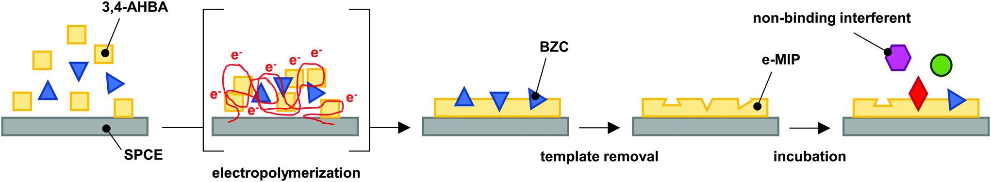 | ||
| Fig. 1 Schematics of the e-MIP development, adapted from literature.26 | ||
2.4. Electrochemical SWV measurements
Electrochemical measurements were performed by SWV after electrode incubation for 30 minutes at ambient temperature in 10 mL of BZC solutions of different concentrations. The supporting electrolyte was 0.04 mol L−1 PBS. SWV was performed in the potential range from +0.5 to +1.5 V, at a frequency of 25 Hz, pulse amplitude of 20 mV, and step potential of 2.5 mV.The functionality of the fabricated MIP sensor was additionally investigated by performing tests on synthetic human urine samples spiked with BZC (0.010–0.50 μmol L−1). Incubation was performed in urine samples diluted with PBS in the ratio of 1:10 for 30 minutes, followed by SWV detection of BZC. Recovery tests were performed on solutions with BZC concentrations of 0.02, 0.25, and 0.5 μmol L−1. Cocaine samples were diluted in PBS before analysis, no other sample pre-treatment was required.
All measurements were performed at room temperature (ca. 25 °C).
2.5. Cocaine samples
Samples in the BFP were analyzed as follows: infrared spectroscopy (FTIR/ATR – Nicolet iS10 model, equipped with a SMART iTR accessory) and classical spot tests were used to establish the cocaine form (base or hydrochloride salt). Quantification analyses were carried out in an Agilent Technologies 6890N gas chromatograph with a flame ionization detector, using an Agilent Technologies 7683B Series autosampler. The chromatographic conditions were: injection volume: 1.0 μL; split ratio 50:1; column: RXi-1MS Methyl Siloxane, 25 m × 200 μm (i.d.) × 0.33 μm film thickness; oven temperature program: 150 °C for 2 min, 40 °C min−1 to 315 °C for 4.5 min; injection port temperature: 280 °C; FID temperature: 320 °C; carrier gas flow rate: 1.0 mL min−1 (helium). The major components cocaine, cis- and trans-cinnamoylcocaine and pharmaceutical cutting agents/adulterants (BZC, phenacetin, caffeine, lidocaine, levamisole, hydroxyzine, procaine, and diltiazem) were quantified using a GC-FID method.48
The data set was composed of 7 seized samples of cocaine hydrochloride and freebase originated from seizures performed by the BFP in different parts of Brazil in 2014. All samples were sent to the Forensic Chemistry Lab at the National Institute of Criminalistics in Brasília, to be analysed in the context of the PeQui Project.49 The samples’ composition is shown in Table S1 in the ESI.†
2.6. Theoretical simulation
Monte Carlo simulation was performed using the DICE program.50 Initial parametrization of the BZC and 3,4-AHBA molecules was made with the use of the LigParGen web server,51–53 and dihedral non-bonded interactions were later reparametrized according to the potential energy curves of a rigid scan of their rotations obtained by DFT single-point calculations, at the B3LYP54,55/6-31G(d,p)56,57 level of theory and D3(BJ) dispersion correction,58,59 as implemented in the Gaussian'09 suite.602.7. Chemometric analysis
Chemometrical analyses were performed using unsupervised methods, called principal component analysis (PCA). It was performed using Statistica 13.0 (Dell, USA) software. To achieve an analysis in which all the information from the SWV (current values from each voltammogram obtained in the analysis of each of the contaminant standards) was used. PCA was the character not to discard any samples or features (variables, the current values for the voltammogram). Instead, it reduces the overwhelming number of dimensions by constructing principal components (PCs). PCs describe variation and account for the varied influences of the original characteristics, the projection of the PC's necessary information. Such results, or loadings, can be traced back from the PCA plot to determine what produces the differences among clusters. Additionally, the Score Plot displays a plot of this projection in the PCs. Using this plot is possible to assign and compare the relative contributions between sample groups.3. Results and discussion
3.1. Electrochemical oxidation of BZC
It has been known for more than a decade that BZC is electrochemically active;61 however, there is limited information in the literature concerning its electrochemical oxidation mechanism. Chemical oxidation of BZC has previously been reported to result in a radical cation via single electron oxidation at the aniline-like group, R-NH2; under acidic conditions nucleophilic attack by an un-oxidized BZC, followed by proton loss, resulted in the ortho-dibenzocaine dimer,62 whereas under alkaline conditions subsequent oxidation and attack by OH− was suggested to result in conversion of R-NH2 to R-NO2.3 Direct electrochemical oxidation of BZC at poly-hematoxylin films at pH 12.2 was also suggested to convert R-NH2 to R-NO2, followed by electrochemical destruction >2 V,63 whereas oxidation at graphite of solid particles of BZC resulted in quasi-reversible voltammetry at pH 2, suggested to be one-electron oxidation to the radical cation at R-NH2.64 Therefore, an initial study of BZC's voltammetric behaviour was conducted, using a GCE in a standard electrochemical cell.An initial study of 100 μmol L−1 BZC in PBS (pH 7.4, Fig. S4 in the ESI†) demonstrated one pronounced oxidation peak; no corresponding reduction feature was observed over the range of investigated scan rates (from 10 to 200 mV s−1). The peak currents (ip) were proportional to the square root of the scan rate, suggesting a diffusion-controlled process,65 with ip (in μA) = (5.3 ± 0.3)v0.5 (in V0.6s−0.5) − (0.25 ± 0.06), r2 = 0.993 (inlay of Fig. S4 in the ESI†).65 Moreover, the slope of the logarithm of the scan rate vs. the logarithm of peak current (0.43) is close to 0.5, which is expected for diffusion-limited systems.66–68
Next, the voltammetric oxidation of BZC was investigated in the pH range 1.0–12.0, using a universal buffer solution as supporting electrolyte (Fig. S5 in the ESI†). As can be observed in Fig. S5,† the single oxidation feature at pH 7 separated into two distinct oxidation processes from pH ≤ 5, whereas pH ≥ 11 a secondary, very significant oxidation process appeared. The latter observation is consistently with the reported electrochemical destruction of BZC at pH 12.2,63 whereas the former is consistent with more stable radical cation intermediates being reported pH < 7.62,64 Oxidation to a radical cation, followed by secondary oxidation of a dibenzocaine dimer62 at a higher potential is consistent with these observations. Conversely, the oxidation of R-NH2 to R-NO2 is also multistep process, passing through R-NHOH and R-NO intermediates,63 and this could explain the two features observed at pH ≤ 5. While further detailed analysis is required to identify the precise mechanism(s), the single oxidation peak observed at pH 7.4 PBS in Fig. S4† is suggested to correspond to an overlap of a number of distinct electrochemical and chemical processes. Nevertheless, since oxidation of BZC in PBS at 50 mV s−1 resulted in a well-defined, single oxidation peak, these conditions were taken forward for the direct electroanalytical quantification of BZC.
3.2. Development of the e-MIP
The electropolymerization process to make a BZC-templated MIP was then performed by running multiple CVs cycles in an optimized solution containing 3,4-AHBA and BZC (Fig. S2†), as monomer and template, respectively. The absence of the reduction peak in the reverse scan shows that the process is irreversible. Furthermore, a significant drop of current corresponding to the main oxidation peak (peak potential at ca. +0.99 V) was observed during the second scanning cycle, suggesting considerable efficiency of the polymerization process, and pronounced surface coverage. The current reduction trend continues with the number of cycles, and converged to zero, meaning that the surface was fully saturated with a non-conductive polymer film. BZC was also likely completely oxidized during the electropolymerization process; however, while scanning in the presence of BZC alone could not form a MIP, the presence of 3,4-AHBA did result in a BZC-selective MIP after template removal (as shown later). The procedure for the template removal from the MIP was performed by running multiple CV scans in PBS with subsequent SWV measurement to ensure that no BZC remained within the molecularly imprinted cavities (cf. Fig. S7 in the ESI†). The electrochemical removal of the template is, in general, faster than solvent elution, that may take several hours.69The overall process of the MIP sensor development was studied by way of CV (Fig. 2A) and EIS (Fig. 2B) after each fabrication step, using 2.0 mmol L−1 [(Fe(CN)6)]3− and 0.1 mol L−1 KCl solution as the test solution. The expected reversible voltammetric features of [(Fe(CN)6)]3−(ref. 65) were observed at the bare GCE. However, upon the formation of BZC-templated 3,4-AHBA-derived polymer layer (or MIP) on the GCE's surface, the current significantly decreased and the redox processes were completely removed. However, a non-imprinted polymer (NIP) layer achieved by polymerizing 3,4-AHBA in the absence of BZC retained much of the [(Fe(CN)6)]3− voltammetric features. Therefore, the NIP was non-electroactive whereas the MIP was completely insulating; it is not clear to authors why this occurs but one of the reasons may be the considerably lower thickness of NIP compared to MIP (as it will be showed subsequently); the presence of BZC therefore assists in the goal of forming a MIP, namely, to make it insulating relative to all molecules except the template. The potential non-innocent role of BZC in the film formation (e.g. beyond templating) does require further, more detailed investigation. Then, when incubating the MIP with 100 μmol L−1 BZC and scanning >+0.6 V resulted in the oxidation of BZC, indicating the MIP was successfully excluding non-specific molecules like [(Fe(CN)6)]3−, but displayed the desired voltammetric response to BZC. In the EIS analysis, the bare GCE displayed the expected lowest resistance when compared to the MIP after polymerization, after the template removal and after incubation.
 | ||
| Fig. 2 Monitoring of the sensor fabrication protocol: (A) CVs from −0.2 to +0.6 V at a scan rate of 10 mV s−1 using 2.0 mmol L−1 of [(Fe(CN)6)]3− in 0.1 mol L−1 KCl in PBS: bare GCE, GCE-MIP after electropolymerization, GCE-MIP after template removal by the means of multicycle CV, GCE-MIP after incubation with 100 μmol L−1 BZC buffer solution, GCE-NIP, and GCE-NIP after “incubation” with 100 μmol L−1 BZC buffer solution. (B) EIS measurements were performed at the fixed potential of +0.14 V, in the frequency range of 0.1 MHz to 0.1 Hz and AC amplitude of 20 mV, using the probe solution consisting of 5.0 mmol L−1 of [(Fe(CN)6)]3− in 0.5 mol L−1 KCl in water: bare GCE, GCE-MIP after electropolymerization, GCE-MIP after template removal by the means of multicycle CV, GCE-MIP after incubation with 50 μmol L−1 BZC buffer solution. | ||
The sensor fabrication protocol was subjected to a systematic optimization of its experimental variables, namely template concentration, number of the CV cycles, applied scan rate during the electropolymerization, and incubation time (Fig. S8 in the ESI†). The main criteria to pick the optimal conditions were the peak current's intensity obtained during the sensor testing by means of SWV after incubation with 30 μmol L−1 BZC in buffer, along with the resolution of the obtained signal. Initially, a template/functional monomer ratio study was performed, which showed the best signal was achieved by a high ratio of BZC, the 3,4-AHBA/BZC ratio of 1:6 was the optimum of all tested; 1:6 ratio was a considerably better than 1:5 and 1:7, and much better than 1:3 and 1:4. Similarly, a scan rate study showed that the optimal value was achieved in a very narrow range, with the best peak current value obtained for the sensor electropolymerized being 10 cycles at 50 mV s−1 (other scan rates tested were 10, 25, 75 and 100 mV s−1). The study on the number of cycles for electropolymerization demonstrated one of the main benefits of the proposed method, i.e. a drastic reduction of the average fabrication time in comparison to bulk or precipitation polymerization. As expected, the increase in the number of the cycles led to a significant increase in the peak currents up to 20 cycles (following the testing of 5 and 10 cycles), but a diminishing signal was observed after 20 cycles. For the sake of the experiment's overall time reduction, further analyses were performed only with 10 electropolymerization cycles, considering the already considerable high values of peak current obtained by 10 scans. Finally, an incubation time study was performed, which showed an exponential rise of the peak currents during incubation times from 5 to 15 minutes before reaching a signal saturation between 15- and 30-minute incubation time.
3.3. Theoretical studies
To further rationalize the e-MIP's interaction with the target molecules and interferents, a combined Monte Carlo-Quantum Chemistry protocol for a realistic simulation of the e-MIP's synthesis was also developed. Taking as an initial premise the widely assumed hypothesis that the molecular imprinting process is driven by the formation of the pre-polymerization complex between the analyte and the building monomers in solution,70–73 the analyte-monomer interaction between the BZC and the 3,4-AHBA was simulated in a water solution with a Monte Carlo methodology. This method allows one to take advantage of the ergodic character of equilibrium systems to survey the conformational space of the pre-polymerization complex, sampling not only the most likely conformation, but also relative populations of different conformers which may have a significant role in the total ability of the 3,4-AHBA polymer to selectively bind to BZC molecules, as well as its relative behaviour to the interferents. It was later tested the most stable of the obtained cavities against the procaine molecule, the second-best binder to the polymer.The production simulation consisted of 585000 steps run in an isothermic-isobaric ensemble, often called a NPT (constant Number of atoms, pressure and temperature) ensemble, after a 230000 steps thermalization. The first 30000 thermalization steps were made with rigid molecules, while in the subsequent 800000 steps only the water molecules were kept rigid. It was later considered the last 385000 steps for the survey of the pre-polymerization process. A box simulating the polymer–water interface, with the BZC molecule at the frontier between the systems – representing the interaction of the molecule with polymer cavities which would not entrap it after polymerization – was built using 1 BZC molecule, 489 3,4-AHBA molecules and 5079 water molecules. Configurations containing the first solvation shell were extracted from a total of 7700 configurations – one for each 50 simulation steps. It was observed that the first solvation shell contained a maximum of 6 3,4-AHBA monomers interacting directly with the BZC molecule, and from the total of 7700 configurations this was the case for 935 configurations. These were then chosen for a clustering analysis according to a hierarchical clustering method based on the unweighted pair group method with arithmetic mean (UPGMA),74 from which we obtained a total of 31 configurations clustered by a distance of 7.5 Angstroms in a distance matrix of the root-mean-square deviation (RMSD) of the atomic coordinates (all coordinates obtained are displayed as ESI†).
These 31 cavities had their geometry optimized using Grimme's GFN2-xTB method.75 This and all subsequent calculations were performed with the ORCA 4.0 package76,77 and the SMD implicit solvent model, with water as solvent.78 The total RMSD difference of the resulting cavities was then analysed and 10 cavities, within a maximum RMSD of 5.3 Angstroms from one another were finally chosen for a higher-level optimization and bond energy evaluation at the BP8679/def2-SVP80 level of theory and RI approximation81,82 and D3(BJ) dispersion. All of them had their minimum stationary points confirmed by frequency calculations (zero imaginary frequencies), which also provided the thermal corrections needed for the evaluation of their enthalpies. The real prevalence of these 10 cavities in the polymer was evaluated according to their formation energies, that is, the difference between the final enthalpy of the complex between BZC and six 3,4-AHBA monomers and the sum of the enthalpies of the same molecules as obtained by a relaxed optimization at the same level of theory. Only 2 of those cavities were found to have significant Boltzmann populations, being within a 1 kcal mol−1 difference from one another regarding their formation enthalpy in the presence of the BZC molecule. Those 2 cavities were finally tested against the procaine molecule by a relaxed optimization and the same level of theory. The images were produced with the VMD program83 and the results are shown in Fig. S9 in the ESI† and Fig. 3. Fig. S9† displays the 8 cavities that were not tested against the procaine molecule, to increase the formation energy, while Fig. 3 displays the two most stable cavities along with their procaine-bound counterparts. The most stable cavity, J-B (Fig. 3) has formation energy of 111.6 kcal mol−1, and is 0.7 kcal mol−1 stabler than cavity I-B. One would expect from these energy differences that cavity I would have less than a third of the cavity J population, and cavity J would dominate selectivity. One may observe that four types of interactions are present in the cavities: hydrogen bonding between the 3,4-AHBA monomers, hydrogen bonding between the monomers and the BZC's amine group π–π stacking between the monomers and the monomers and the BZC molecule. Formation enthalpy initially increases as the number of hydrogen bonds between the monomers increase. Cavities A-D show an increasing packing of the monomers around the BZC molecule along with the formation of multiple hydrogen bonds between 3,4-AHBA's hydroxyl, carboxyl and amine groups, leading to progressively increasing stability. As one may see, the most stable cavities in Fig. S9,† cavities F–H, show a common feature: two hydrogen bonds between the monomers’ and BZC's amine groups, and the alignment between the BZC's and 3,4-AHBA's aromatic systems, resulting in π–π stacking. In Fig. 3, the two most stable cavities differ in two aspects. Cavity J, the most stable, has three BZC-monomer hydrogen bonds, and BZC is part of a three-layer stacking with two other monomers, instead of just one as in cavity I. One may observe that the cavity J offers only slightly more stability to the procaine molecule than to the BZC, in agreement with the experimental trends. The procaine molecule shows a much larger affinity for the less abundant I cavity, which is less rigid and allows for better accommodation of the procaine's aromatic system, which must be distorted in the J cavity. One should further take notice of the cavities’ structural integrity. All the main interactions between monomers and the procaine's primary amine and aromatic groups and the monomers are maintained even with a thoroughly relaxed optimization with both BZC and procaine, strongly suggesting the cavities are real structural minima of the pre-polymerization complex.
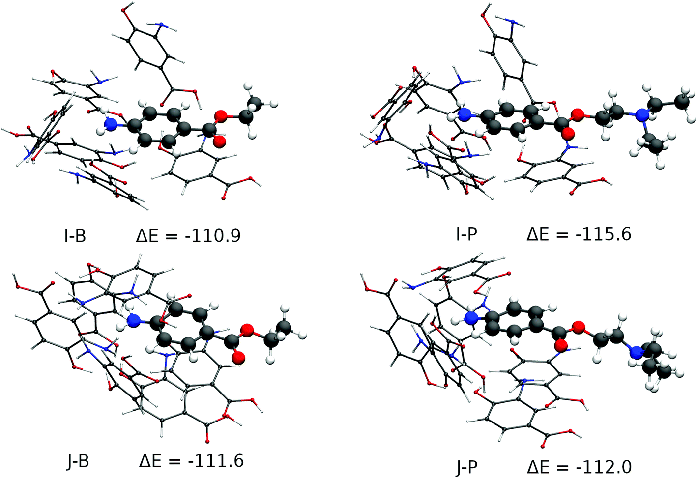 | ||
| Fig. 3 Top left: second most stable cavity formed around BZC; top right: when BZC is substituted by procaine; bottom left: most stable of all cavities formed around BZC; bottom right: when BZC is substituted by procaine (energies in kcal mol−1). B stands for BZC and P stands for procaine. | ||
According to theoretical simulation the driving force behind the MIP's selectivity appears then to be an arrangement of 3,4-AHBA monomers, bound between themselves by strong hydrogen bonds and also by π–π stacking, in such a manner that two interactions with BZC are maximized: hydrogen bonds to its amine group, and stacking with its aromatic system, which extends to the ester group. The best and most abundant cavity in these conditions would be J, which is slightly selective to procaine – procaine being 0.4 kcal mol−1 more stable in the cavity than BZC. Secondary cavities such as I, which have only two aromatic systems stacked and two hydrogen bonds with the amine group, have even stronger selectivity towards procaine, but much smaller populations in the pre-polymerization complex, and close selectivity to both BZC and procaine by the MIP as a whole will be dominated by energy differences in the dominant J cavity (Fig. 3). The combined Monte Carlo-Quantum Chemistry protocol is shown to be capable of accounting for the diversity of phenomena in the realistic MIP formation environment, and as such, for the rational design of MIPs for other targets, which are under investigation.
3.4. Analytical application
Having understood the MIP selectivity a bit more, the optimized GCE-MIP sensor was then tested for the electroanalytical quantification of BZC. This GCE-MIP sensor gave a linear response up to 100 μmol L−1 BZC, although there was some background noise when the measurements were in the nA level, the calibration curve had the following analytical parameters: r2 of 0.9991, ip (μA) = (192 ± 3) [BZC] (nmol L−1) + (2.8 ± 0.2), and coefficient of variation of 7.9% (Fig. 4). The slope of the calibration curve was around 100 times large than the corresponding NIP: ip (μA) = (2.0 ± 0.2) [BZC] (nmol L−1) + (0.01 ± 0.01). Additionally, the developed GCE-MIP sensors were subjected to repeatability and reproducibility studies, both were based on deviations in peak current, by dividing the standard deviation by the average. A repeatability value of 5% was obtained by intra-day analysis (n = 5) of a 100 μmol L−1 BZC solution using the same sensor. A reproducibility value of 9% was determined by inter-day measurements (n = 5) of a 100 μmol L−1 BZC solution, each time by using a newly fabricated GCE-MIP device. In both cases the incubation time was limited to 20 minutes. The e-MIP appears to deteriorate overnight if kept in a desiccator. Thus, stability would be an important issue to tackle when making the technology transfer from the central police laboratory to other location, like airport customs or international borders.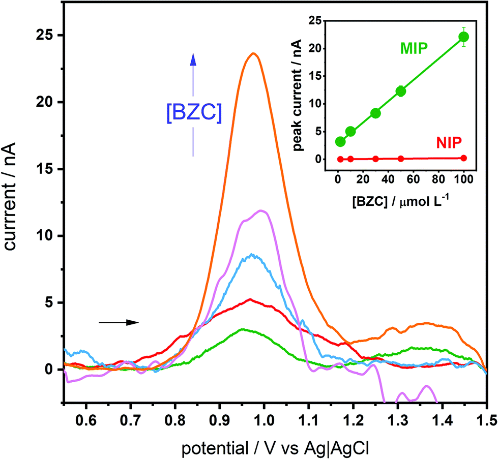 | ||
| Fig. 4 SWVs of BZC in PBS (2, 10, 30, 50 and 100 μmol L−1), detected using the optimized GCE-MIP sensing device (potential range from +0.5 to +1.5 V, at a frequency of 25 Hz, pulse amplitude of 20 mV and step potential of 2.5 mV, baseline correction with moving average level 2). Inlay: the corresponding calibration curve and the calibration curve for the NIP. | ||
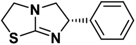
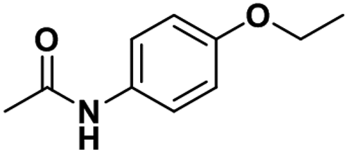
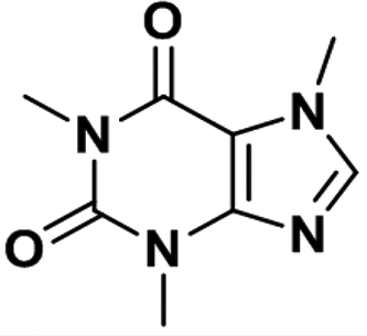
The selectivity of the optimized GCE-MIP device was then investigated, comparing BZC to seven structurally similar heterocyclic compounds, namely caffeine, phenacetin, levamisole, lidocaine, aminopyrine, procaine and hydroxyzine. It is worth mentioning that some of these compounds are also commonly used as the “cutting” additives in street-distributed drug samples, like BZC. For this purpose, 30 μmol L−1 solutions of each analyte in PBS were used, while the incubation time was kept at 45 minutes. This study's obtained results are presented in Table 2, including the so-called selectivity factor (α), which was calculated by dividing the BZC peak current by the interferent's peak current. Firstly, it can be observed that the peak potentials corresponding to the possible interferents vary when compared to the BZC peak potential. Additionally, based on α, only hydroxyzine and procaine could significantly compromise BZC analysis and yield a positive result. However, taking into consideration that their peak potentials are shifted towards different potentials than BZC, one should be able to differentiate their signal from a pure BZC signal. The similar affinity for BZC and hydroxyzine compounds is related to the main driving forces in the formation of the pre-polymerization complex: hydrogen bonding to the BZC's amine group and π–π stacking between BZC's aromatic system and the 3,4-AHBA monomers. In fact, hydroxyzine is the compound with the largest affinity for the polymer, and it has a chlorine replacing the amine group playing a double role: while it is able to also accept hydrogen bonds from the polymer, it is also able to direct electron density towards the aromatic system, contributing to its interaction with the stacked monomers. On the other hand, the aminopyrine molecule is the fourth with the largest affinity, just below BZC itself. It has no group analogue to BZC's amine but features a pyrazolone attached to the benzene ring that is able to interact with it by hyperconjugation, maintaining a planarity similar to the carboxyl-benzene system in BZC and thus also allowing for π–π stacking with the 3,4-AHBA monomers. It is interesting to note, and even analytically exploitable, that the compounds peaks’ potentials are different with the GCE-MIP that those obtained with a bare SPCE 2 or a boron-doped diamond electrode (BDDE).84 In particular, with the GCE-MIP it seems more possible to distinguish BZC (+0.92 V) from procaine (+0.97 V), whereas with the BDDE both had a peak potential of +1.1 V, and with the bare SPCE both had a peak potential of +0.9 V. Additionally, with the GCE-MIP lidocaine has a peak potential of +0.87, which with the SPCE would be difficult to differentiate.
| Compound | Structure | Peak potential/V | Peak current/μA | α |
|---|---|---|---|---|
| Hydroxyzine |
|
0.83 ± 0.03 | 0.67 ± 0.02 | 0.94 |
| Procaine |
|
0.89 ± 0.03 | 0.67 ± 0.02 | 0.94 |
| BZC |
|
0.96 ± 0.03 | 0.63 ± 0.02 | 1.0 |
| Aminopyrine |
|
0.94 ± 0.03 | 0.48 ± 0.02 | 1.3 |
| Lidocaine |
|
0.87 ± 0.03 | 0.23 ± 0.02 | 2.7 |
| Levamisole |
|
0.92 ± 0.03 | 0.21 ± 0.02 | 3.0 |
| Phenacetin |
|
0.84 ± 0.03 | 0.19 ± 0.02 | 3.3 |
| Caffeine |
|
0.97 ± 0.03 | 0.07 ± 0.02 | 9 |
The optimized GCE-MIP sensor was applied in the detection of BZC in spiked synthetic urine samples, with a concentration range from 0.010 to 0.50 μmol L−1 (Fig. S10 in the ESI†), resulting in an excellent linear relationship between BZC concentration and current, with r2 of 0.997. The analysis of BZC in urine can be of clinical relevance, including in cases of cocaine consumption.85 The limit of detection (LOD) and limit of quantification (LOQ) were calculated as three and ten times the standard deviation of the intercept/slope, respectively, giving a LOD of 2.9 nmol L−1 and LOQ of 9.8 nmol L−1. To the best of the authors’ knowledge this is the one of the lowest LODs reported for the electroanalytical quantification of BZC so far, only a work by Reddy and co-workers achieved the detection of a slightly lower concentration,61 as shown comparatively in Table 1.
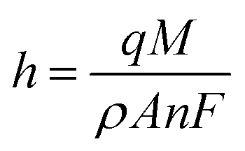
Subsequently, to develop a portable e-MIP sensing platform for use in the swift profiling of drugs in the BFP's laboratory, the GCE was replaced with disposable screen-printed carbon electrodes (SPCE). The optimized conditions were then employed to form the MIP on the surface of these SPCE, which yielded similar voltammetric responses as observed on the GCE. The surface of the sensor was further characterized by scanning electron microscopy (SEM) (Fig. 5). Given the inherent roughness of the bare SPCE there were no observable differences between the MIP, NIP and the bare SPCE. This suggests that the formed polymeric film is very thin, which is consistent with the calculated film thicknesses of 77 ± 3 nm for the MIP and 33 ± 3 nm for the NIP. These film thicknesses were estimated according to the following equation:86,87
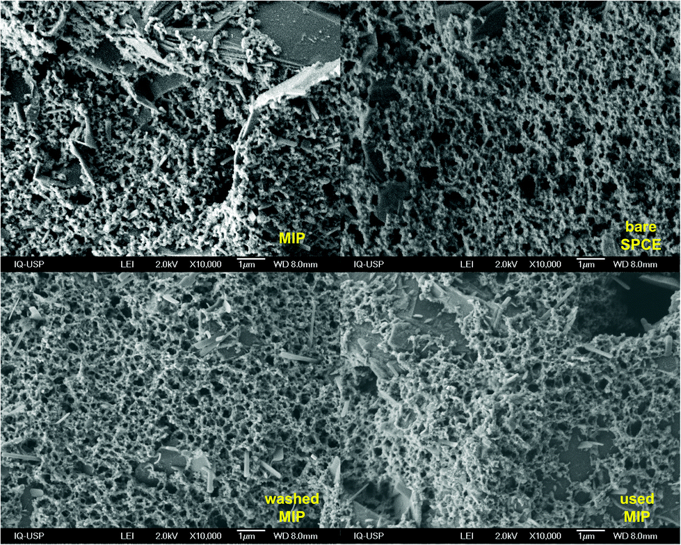 | ||
| Fig. 5 SEM micrographs of SPCE with and without MIP film. | ||
The SCPE-MIPs were next employed for analysis of 7 seized “cocaine” samples. These samples were known to include different quantities of BZC and cocaine (both from almost none to above 50% m m−1 concentrations), as well as several interferences used in the selectivity studies, such as phenacetin, caffeine, aminopyrine and lidocaine, and a range of unknown components (Table S1 in ESI†). SWV profiling of the 7 samples was achieved with the SPCE-MIPs using the samples dissolved in PBS (15 mg L−1). As can be seen in Fig. 6, each of the seven samples produced numerous distinguishable voltammetric signals; these numerous features prevented the voltammetric quantification of BZC or cocaine, though both their signal was detected. However, voltammetric fingerprinting of the various interferences indicated these were present in the SWV using the e-MIP.
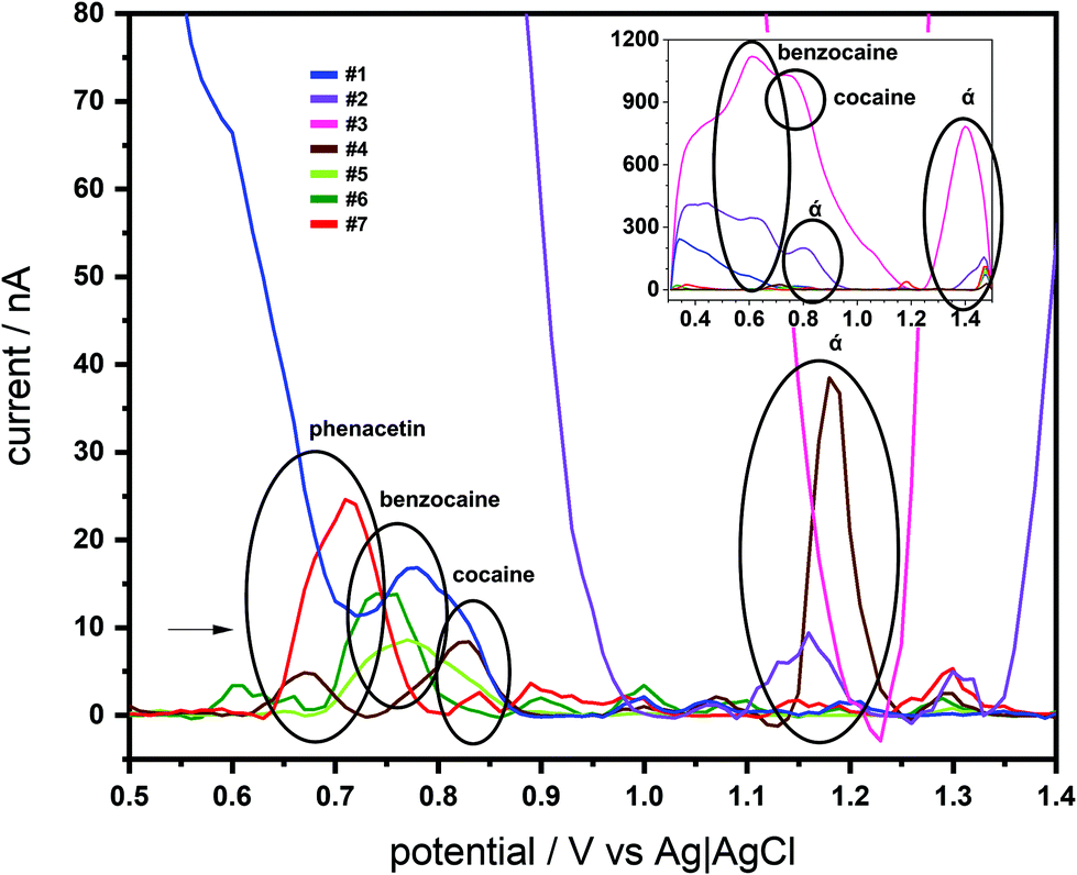 | ||
| Fig. 6 Electrochemical profile of the samples acquired by the BFP measured in the SPCE-MIP device through SWV of each sample in PBS (potential range from +0.5 to +1.5 V, at a frequency of 25 Hz, pulse amplitude of 20 mV and step potential of 2.5 mV). | ||
Since the voltammetric information was a lot of data to be interpreted, PCA was used to evaluate the possibility, as a proof-of-concept, of discriminating the know contaminants in the cocaine samples. Hence, all the current values of the SWV recorded were used in this discrimination procedure. To obtain a better discrimination, it is normally used in the literature more than 70% of total variance explained (sum of percentage of information described in the PCs). Hence, the proposed work used 3 PCs to obtain 81.8%, indicating a large amount of original information described in the discrimination process. From Fig. 7 (the score plot of the proposed discrimination using PCA), it is possible to see that the location of the contaminants is in different regions of the 3D plots. BZC is separated in the positive quadrant of the PC1 and PC2 and distinguished from procaine using the PC3 information. Additionally, the aminopyrine is the only adulterant in the PC2 positive region and PC1 negative region. The hydroxyzine is the only contaminant in the negative area of the PC1 positive and PC2 negative quadrant. Lidocaine, levamisole, caffeine, and phenacetin reported in the PC1 negative – PC2 negative quadrant and PC3 component discriminated caffeine and phenacetin from lidocaine levamisole. The discrimination between these two groups, lidocaine and levamisole and caffeine and phenacetin, could be more complicated than voltammetric behaviour. Still, some dual detection devices could be used to add more information to the discrimination process.89 Hence, the result demonstrates proof-of-concept that SPCE-MIP SWV could be employed as a rapid forensic fingerprinting analysis of narcotics.
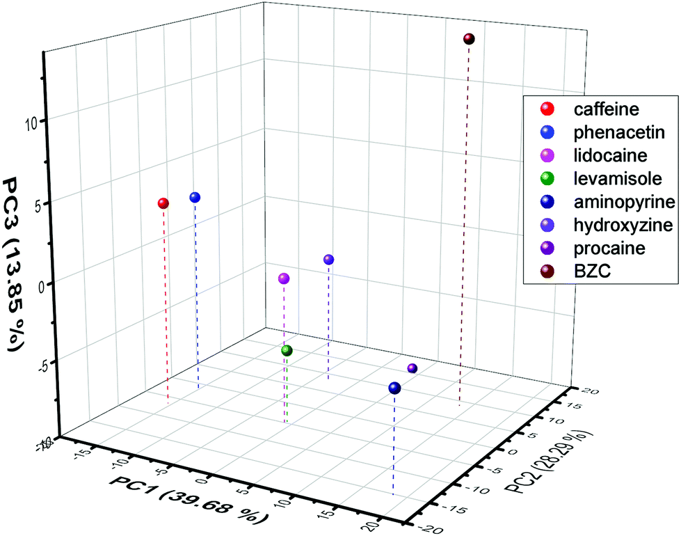 | ||
| Fig. 7 PCA score plot obtained from the SWV current values extracted from each electrochemical experiment performed for each contaminant. | ||
The last Scientific Working Group for the Analysis of Seized Drugs (SWGDRUG) recommendations90 divide the analytical methods for drugs into 3 categories with different levels of selectivity: A – “Selectivity through structural Information” (e.g. mass spectrometry); B – “selectivity through chemical and physical characteristics” (e.g. UV-Vis spectroscopy); and C – “selectivity through general or class information” (e.g. spot tests). Then, two combinations of techniques are accepted as the minimum suitable identification, using (1) A+(A or B or C), and (2) B+B+(B or C). At the moment, electrochemical techniques are not part of the options. The authors advocate that a properly validated electroanalytical methodology should be included in the category B, since it can provide specific electrochemical information to identify forensic analytes; the results presented here represent a significant step in this direction.
4. Conclusions
An e-MIP sensor was developed by electropolymerization of the monomer 3,4-AHBA on a carbon surface in the presence of BZC. Experimental parameters affecting the sensor's performance were studied and optimized. DFT theoretical studies were performed to better understand the interactions between the MIP and the analytes. Results confirmed the suitability of the proposed sensor for the swift electroanalytical determination of the template BZC in human urine, showing it as a promising tool for medical and forensic analysis. Proof-of-principle was also demonstrated on how this system can help the in situ rapid identification of seized drugs’ provenience. Future work should be focused on creating a long-time stable e-MIP associated with a robust software to be used by less qualified users.Author contributions
Conceptualization: NT, AACB, AOM, TRLCP, and LMG; data curation: AL, BMJ, NT, AACB, LA, TRLCP, and LMG; formal analysis: RAG, AL, BMJ, NT, AACB, LA, TRLCP, and LMG; funding acquisition: AACB, TRLCP, and LMG; investigation: RAG, AL, BMJ, NT; methodology: RAG, AL, BMJ, NT, AACB, LA, TRLCP, and LMG; project administration: AACB, AOM, TRLCP, and LMG; resources: AACB, AOM, TRLCP, and LMG; supervision: AACB, AOM, TRLCP, and LMG; validation: RAG, AL, NT; visualization: AL, NT, LMG; writing – original draft: AL, BMJ, NT, LMG; writing – review & editing: RAG, AL, BMJ, NT, AACB, AOM, LA, TRLCP, and LMG.Conflicts of interest
All authors declare no conflicts of interest.Acknowledgements
This work was supported by Fundação de Amparo à Pesquisa do Estado de São Paulo (FAPESP – 2019/05569-8, 2018/14425-7, 2019/11214-8, 2018/ 08782-1, 2018/13922-7, 2014/25770-6, and 2015/01491-3), Conselho Nacional de Desenvolvimento Científico e Tecnológico (CNPq – 117865/2019-2, 465768/2014-8, and 309715/2017-2), and Coordenação de Aperfeiçoamento de Pessoal de Nível Superior (CAPES – 001, 3359/2014 Pró-Forenses Edital 25/2014). Authors would like to thank Professor Maria del Pilar Taboada Sotomayor (UNESP, Araraquara – SP, Brazil) for the kind gift of 3,4-AHBA for the initial experiments.References
- E. De Rycke, C. Stove, P. Dubruel, S. De Saeger and N. Beloglazova, Biosens. Bioelectron., 2020, 169, 112579 CrossRef CAS.
- M. de Jong, N. Sleegers, J. Kim, F. Van Durme, N. Samyn, J. Wang and K. De Wael, Chem. Sci., 2016, 7, 2364–2370 RSC.
- S. Plotycya, O. Strontsitska, S. Pysarevska, M. Blazheyevskiy and L. Dubenska, Int. J. Electrochem., 2018, 2018, 1–10 CrossRef.
- L. Shaw and L. Dennany, Curr. Opin. Electrochem., 2017, 3, 23–28 CrossRef CAS.
- D. E. Becker and K. L. Reed, Anesth. Progr., 2006, 53, 98–109 CrossRef.
- D. G. A. Gondim, A. M. Montagner, I. C. Pita-Neto, R. J. D. S. Bringel, F. A. L. Sandrini, E. F. C. Moreno, A. M. Sousa and A. B. Correia, Int. J. Dent., 2018, 2018, 1–5 CrossRef.
- G. Kagan, L. Huddlestone and P. Wolstencroft, J. Int. Med. Res., 1982, 10, 443–446 CrossRef CAS.
- G. T. Kluemper, D. G. Hiser, M. K. Rayens and M. J. Jay, Am. J. Orthod. Dentofacial Orthop., 2002, 122, 359–365 CrossRef.
- M. O. Salles, W. R. Araujo and T. R. L. C. Paixão, J. Braz. Chem. Soc., 2016, 27, 54–61 CAS.
- T. R. Fiorentin, M. Fogarty, R. P. Limberger and B. K. Logan, Forensic Sci. Int., 2019, 295, 199–206 CrossRef CAS.
- J. P. Smith, J. P. Metters, C. Irving, O. B. Sutcliffe and C. E. Banks, Analyst, 2014, 139, 389–400 RSC.
- S. D. Brandt, H. R. Sumnall, F. Measham and J. Cole, Drug Test. Anal., 2010, 2, 377–382 CrossRef CAS.
- S. Pysarevska, L. Dubenska, S. Plotycya and Ľ. Švorc, Sens. Actuators, B, 2018, 270, 9–17 CrossRef CAS.
- M. A. Mohamed, S. A. Atty, H. A. Merey, T. A. Fattah, C. W. Foster and C. E. Banks, Analyst, 2017, 142, 3674–3679 RSC.
- R. M. F. de Lima, M. D. de Oliveira Silva, F. S. Felix, L. Angnes, W. T. P. dos Santos and A. A. Saczk, Electroanalysis, 2018, 30, 283–287 CrossRef CAS.
- H. Sun, J.-P. Lai, F. Chen and D.-R. Zhu, Anal. Bioanal. Chem., 2015, 407, 1745–1752 CrossRef CAS.
- L. Andersson, B. Sellergren and K. Mosbach, Tetrahedron Lett., 1984, 25, 5211–5214 CrossRef CAS.
- G. Wulff, D. Oberkobusch and M. Minárik, React. Polym., Ion Exch., Sorbents, 1985, 3, 261–275 CrossRef CAS.
- P. S. Sharma, A. Pietrzyk-Le, F. D'Souza and W. Kutner, Anal. Bioanal. Chem., 2012, 402, 3177–3204 CrossRef CAS.
- J. J. BelBruno, Chem. Rev., 2019, 119, 94–119 CrossRef CAS.
- J. G. Pacheco, P. Rebelo, F. Cagide, L. M. Gonçalves, F. Borges, J. A. Rodrigues and C. Delerue-Matos, Talanta, 2019, 194, 689–696 CrossRef CAS.
- G. A. Ruiz-Córdova, S. Khan, L. M. Gonçalves, M. I. Pividori, G. Picasso and M. D. P. T. Sotomayor, Talanta, 2018, 181, 19–23 CrossRef.
- R. A. S. Couto, S. S. Costa, B. Mounssef, J. G. Pacheco, E. Fernandes, F. Carvalho, C. M. P. Rodrigues, C. Delerue-Matos, A. A. C. Braga, L. M. Gonçalves and M. B. Quinaz, Sens. Actuators, B, 2019, 290, 378–386 CrossRef CAS.
- R. R. Pupin, M. V. Foguel, L. M. Gonçalves and M. D. P. T. Sotomayor, J. Appl. Polym. Sci., 2019, 137, 48496 CrossRef.
- M. M. Pedroso, M. V. Foguel, D. H. S. Silva, M. D. P. T. Sotomayor and H. Yamanaka, Sens. Actuators, B, 2017, 253, 180–186 CrossRef CAS.
- L. M. Gonçalves, Curr. Opin. Electrochem., 2021, 25, 100640 CrossRef.
- A. Lobato, E. A. Pereira and L. M. Gonçalves, Talanta, 2021, 221, 121546 CrossRef CAS.
- R. A. S. Couto, B. Mounssef, F. Carvalho, C. M. P. Rodrigues, A. A. C. Braga, L. Aldous, L. M. Gonçalves and M. B. Quinaz, Sens. Actuators, B, 2020, 316, 128133 CrossRef CAS.
- I. Benachio, A. Lobato and L. M. Gonçalves, J. Mol. Recognit., 2021, e2878 Search PubMed.
- A. Merkoçi and S. Alegret, Trends Anal. Chem., 2002, 21, 717–725 CrossRef.
- A. H. A. Hassan, S. L. Moura, F. H. M. Ali, W. A. Moselhy, M. D. P. T. Sotomayor and M. I. Pividori, Biosens. Bioelectron., 2018, 118, 181–187 CrossRef CAS.
- S. Khan, A. Wong, M. V. B. Zanoni and M. D. P. T. Sotomayor, Mater. Sci. Eng., C, 2019, 103, 109825 CrossRef CAS.
- A. Adumitrăchioaie, Int. J. Electrochem. Sci., 2018, 2556–2576 CrossRef.
- D. Fauzi and F. A. Saputri, Int. J. Appl. Pharm., 2019, 1–6 CAS.
- R. Gui, H. Guo and H. Jin, Nanoscale Adv., 2019, 1, 3325–3363 RSC.
- Y. Zhang, W. Huang, X. Yin, K. A. Sarpong, L. Zhang, Y. Li, S. Zhao, H. Zhou, W. Yang and W. Xu, React. Funct. Polym., 2020, 157, 104767 CrossRef CAS.
- J. Drzazgowska, B. Schmid, R. D. Süssmuth and Z. Altintas, Anal. Chem., 2020, 92, 4798–4806 CrossRef CAS.
- A. Kushwaha, J. Srivastava, A. K. Singh, R. Anand, R. Raghuwanshi, T. Rai and M. Singh, Biosens. Bioelectron., 2019, 145, 111698 CrossRef CAS.
- F. W. Scheller, X. Zhang, A. Yarman, U. Wollenberger and R. E. Gyurcsányi, Curr. Opin. Electrochem., 2019, 14, 53–59 CrossRef CAS.
- R. D. Crapnell, A. Hudson, C. W. Foster, K. Eersels, B. van Grinsven, T. J. Cleij, C. E. Banks and M. Peeters, Sensors, 2019, 19, 1204 CrossRef CAS.
- A. A. Lahcen and A. Amine, Electroanalysis, 2019, 31, 188–201 CrossRef CAS.
- K. Vinkovic, N. Galic and M. G. Schmid, J. Liq. Chromatogr. Relat. Technol., 2018, 41, 6–13 CrossRef CAS.
- M. C. A. Marcelo, T. R. Fiorentin, K. C. Mariotti, R. S. Ortiz, R. P. Limberger and M. F. Ferrão, Anal. Methods, 2016, 8, 5212–5217 RSC.
- J. C. Carter, W. E. Brewer and S. M. Angel, Appl. Spectrosc., 2000, 54, 1876–1881 CrossRef CAS.
- N. V. S. Rodrigues, E. M. Cardoso, M. V. O. Andrade, C. L. Donnici and M. M. Sena, J. Braz. Chem. Soc., 2013, 24, 507–517 CrossRef CAS.
- USDoS, International Narcotics Control Strategy Report - Bureau for International Narcotics and Law Enforcement Affairs, 2020 Search PubMed.
- J. C. Cueto, BBC news, http://www.bbc.com/portuguese/brasil-51699219, 2020.
- É. D. Botelho, R. B. Cunha, A. F. C. Campos and A. O. Maldaner, J. Braz. Chem. Soc., 2014, 25, 611–618 Search PubMed.
- J. J. Zacca, É. D. Botelho, M. L. Vieira, F. L. A. Almeida, L. S. Ferreira and A. O. Maldaner, Sci. Justice, 2014, 54, 300–306 CrossRef.
- H. M. Cezar, S. Canuto and K. Coutinho, J. Chem. Inf. Model., 2020, 60, 3472–3488 CrossRef CAS.
- L. S. Dodda, J. Z. Vilseck, J. Tirado-Rives and W. L. Jorgensen, J. Phys. Chem. B, 2017, 121, 3864–3870 CrossRef CAS.
- L. S. Dodda, I. Cabeza de Vaca, J. Tirado-Rives and W. L. Jorgensen, Nucleic Acids Res., 2017, 45, W331–W336 CrossRef CAS.
- W. L. Jorgensen and J. Tirado-Rives, Proc. Natl. Acad. Sci. U. S. A., 2005, 102, 6665–6670 CrossRef CAS.
- C. Lee, W. Yang and R. G. Parr, Phys. Rev. B: Condens. Matter Mater. Phys., 1988, 37, 785–789 CrossRef CAS.
- A. D. Becke, J. Chem. Phys., 1993, 98, 5648–5652 CrossRef CAS.
- W. J. Hehre, R. Ditchfield and J. A. Pople, J. Chem. Phys., 1972, 56, 2257–2261 CrossRef CAS.
- M. M. Francl, W. J. Pietro, W. J. Hehre, J. S. Binkley, M. S. Gordon, D. J. DeFrees and J. A. Pople, J. Chem. Phys., 1982, 77, 3654–3665 CrossRef CAS.
- S. Grimme, J. Antony, S. Ehrlich and H. Krieg, J. Chem. Phys., 2010, 132, 154104 CrossRef.
- S. Grimme, S. Ehrlich and L. Goerigk, J. Comput. Chem., 2011, 32, 1456–1465 CrossRef CAS.
- M. J. Frisch, G. W. Trucks, H. B. Schlegel, G. E. Scuseria, M. A. Robb, J. R. Cheeseman, G. Scalmani, V. Barone, B. Mennucci, G. A. Petersson, H. Nakatsuji, M. Caricato, X. Li, H. P. Hratchian, A. F. Izmaylov, J. Bloino, G. Zheng, J. L. Sonnenberg, M. Hada, M. Ehara and D. J. Fox, Gaussian 09, (Revision D.01), Gaussian Inc., Pittsburgh, USA, 2009 Search PubMed.
- T. M. Reddy, K. Balaji and S. R. J. Reddy, Croat. Chem. Acta, 2006, 79, 253–259 CAS.
- B. Marjanović, I. Juranić, G. Ćirić-Marjanović, I. Pašti, M. Trchová and P. Holler, React. Funct. Polym., 2011, 71, 704–712 CrossRef.
- A. Samide, B. Tutunaru, G. Bratulescu and C. Ionescu, J. Appl. Polym. Sci., 2013, 130, 687–697 CrossRef CAS.
- Š. Komorsky-Lovrić, N. Vukašinović and R. Penovski, Electroanalysis, 2003, 15, 544–547 CrossRef.
- N. Elgrishi, K. J. Rountree, B. D. McCarthy, E. S. Rountree, T. T. Eisenhart and J. L. Dempsey, J. Chem. Educ., 2018, 95, 197–206 CrossRef CAS.
- C. Batchelor-McAuley, L. M. Gonçalves, L. Xiong, A. A. Barros and R. G. Compton, Chem. Commun., 2010, 46, 9037–9039 RSC.
- L. M. Gonçalves, C. Batchelor-Mcauley, A. A. Barros and R. G. Compton, J. Phys. Chem. C, 2010, 114, 14213–14219 CrossRef.
- E. M. Tavares, A. M. Carvalho, L. M. Gonçalves, I. M. Valente, M. M. Moreira, L. F. Guido, J. A. Rodrigues, T. Doneux and A. A. Barros, Electrochim. Acta, 2013, 90, 440–444 CrossRef CAS.
- S. Khan, S. Hussain, A. Wong, M. V. Foguel, L. M. Gonçalves, M. I. Pividori and M. D. P. T. Sotomayor, React. Funct. Polym., 2018, 122, 175–182 CrossRef CAS.
- B. Zhang, X. Fan and D. Zhao, Polymers, 2018, 11, 17 CrossRef.
- Y. Han, L. Gu, M. Zhang, Z. Li, W. Yang, X. Tang and G. Xie, Comput. Theor. Chem., 2017, 1121, 29–34 CrossRef CAS.
- X. Li, Y. He, F. Zhao, W. Zhang and Z. Ye, RSC Adv., 2015, 5, 56534–56540 RSC.
- L. S. Fernandes, P. Homem-de-Mello, E. C. de Lima and K. M. Honorio, Eur. Polym. J., 2015, 71, 364–371 CrossRef CAS.
- H. M. Cezar, Clustering Trajectory, https://github.com/hmcezar/clustering-traj (accessed November 2020) Search PubMed.
- C. Bannwarth, S. Ehlert and S. Grimme, J. Chem. Theory Comput., 2019, 15, 1652–1671 CrossRef CAS.
- F. Neese, Wiley Interdiscip. Rev.: Comput. Mol. Sci., 2012, 2, 73–78 CAS.
- F. Neese, Wiley Interdiscip. Rev.: Comput. Mol. Sci., 2018, 8, e1327 Search PubMed.
- A. V. Marenich, C. J. Cramer and D. G. Truhlar, J. Phys. Chem. B, 2009, 113, 6378–6396 CrossRef CAS.
- J. P. Perdew, Phys. Rev. B: Condens. Matter Mater. Phys., 1986, 33, 8822–8824 CrossRef.
- F. Weigend and R. Ahlrichs, Phys. Chem. Chem. Phys., 2005, 7, 3297–3305 RSC.
- F. Weigend, Phys. Chem. Chem. Phys., 2006, 8, 1057–1065 RSC.
- E. Valeyev, Libint - a library for the evaluation of molecular integrals of many-body operators over Gaussian functions, http://libint.valeyev.net (accessed November 2020) Search PubMed.
- W. Humphrey, A. Dalke and K. Schulten, J. Mol. Graphics, 1996, 14, 33–38 CrossRef CAS , 27–8.
- J. M. Freitas, D. L. O. Ramos, R. M. F. Sousa, T. R. L. C. Paixão, M. H. P. Santana, R. A. A. Muñoz and E. M. Richter, Sens. Actuators, B, 2017, 243, 557–565 CrossRef CAS.
- C. D. McKinney, K. F. Postiglione and D. A. Herold, Clin. Chem., 1992, 38, 596–597 CrossRef CAS.
- E. Mathieu-Scheers, S. Bouden, C. Grillot, J. Nicolle, F. Warmont, V. Bertagna, B. Cagnon and C. Vautrin-Ul, J. Electroanal. Chem., 2019, 848, 113253 CrossRef CAS.
- S. A. Zaidi, Electrochim. Acta, 2018, 274, 370–377 CrossRef CAS.
- R. F. Alves, D. L. Franco, M. T. Cordeiro, E. M. de Oliveira, R. A. F. Dutra and M. D. P. T. Sotomayor, Sens. Actuators, B, 2019, 296, 126681 CrossRef.
- W. A. Ameku, W. R. de Araujo, C. J. Rangel, R. A. Ando and T. R. L. C. Paixão, ACS Appl. Nano Mater., 2019, 2, 5460–5468 CrossRef CAS.
- SWGDRUG, Scientific working group for the analysis of seized drugs (SWGDRUG) recommendations - swgdrug.org/approved, 2019 Search PubMed.
- P. Surmann, B. Peter and C. Stark, Anal. Bioanal. Chem., 1996, 356, 192–196 CrossRef CAS.
- I. F. Abdullin, N. N. Chernysheva and G. K. Budnikov, J. Anal. Chem., 2002, 57, 629–631 CrossRef CAS.
- R. T. Kachoosangi, G. G. Wildgoose and R. G. Compton, Electroanalysis, 2008, 20, 2495–2500 CrossRef CAS.
- H. Dejmkova, V. Vokalova, J. Zima and J. Barek, Electroanalysis, 2011, 23, 662–666 CAS.
- T. G. Silva and T. R. L. C. Paixão, in 2017 ISOCS/IEEE International Symposium on Olfaction and Electronic Nose (ISOEN), IEEE, 2017, pp. 1–3 Search PubMed.
- G. Dutu, C. Cristea, B. Ede, V. Harceaga, A. Saponar, E.-J. Popovici and R. Sandulescu, Farmacia, 2011, 59, 147–160 CAS.
- M. Jadach, A. Błazewicz and Z. Fijalek, Acta Pol. Pharm., 2012, 69, 397–403 CAS.
- R. Ramkumar and M. V. Sangaranarayanan, ChemistrySelect, 2019, 4, 9776–9783 CrossRef CAS.
- R. L. Mesa, J. E. L. Villa, S. Khan, R. R. A. Peixoto, M. A. Morgano, L. M. Gonçalves, M. D. P. T. Sotomayor and G. Picasso, Nanomaterials, 2020, 10(12), 2541 CrossRef CAS.
- R. A. S. Couto, L. M. Gonçalves, F. Carvalho, J. A. Rodrigues, C. M. P. Rodrigues and M. B. Quinaz, Crit. Rev. Anal. Chem., 2018, 48(5), 372–390 CrossRef CAS.
Footnote |
| † Electronic supplementary information (ESI) available. See DOI: 10.1039/d0an02274h |
| This journal is © The Royal Society of Chemistry 2021 |