
 Open Access Article
 This Open Access Article is licensed under a Creative Commons Attribution-Non Commercial 3.0 Unported Licence
Intermolecular background decay in RIDME experiments†
Katharina
Keller
a,
Mian
Qi
b,
Christoph
Gmeiner
a,
Irina
Ritsch
a,
Adelheid
Godt
b,
Gunnar
Jeschke
 a,
Anton
Savitsky
c and
Maxim
Yulikov
*a
a,
Anton
Savitsky
c and
Maxim
Yulikov
*a
aLaboratory of Physical Chemistry, Department of Chemistry and Applied Biosciences, ETH Zurich, Vladimir-Prelog-Weg 2, 8093 Zurich, Switzerland. E-mail: maxim.yulikov@phys.chem.ethz.ch
bFaculty of Chemistry and Center for Molecular Materials (CM2), Bielefeld University, Universitätsstraße 25, 33615 Bielefeld, Germany
cPhysics Department, Technical University Dortmund, Otto-Hahn-Straße 4a, 44227, Dortmund, Germany
First published on 20th March 2019
Abstract
The relaxation-induced dipolar modulation enhancement (RIDME) technique allows the determination of distances and distance distributions in pairs containing two paramagnetic metal centers, a paramagnetic metal center and an organic radical, and, under some conditions, also in pairs of organic radicals. The strengths of the RIDME technique are its simple setup requirements, and the absence of bandwidth limitations for spin inversion which occurs through relaxation. A strong limitation of the RIDME technique is the background decay, which is often steeper than that in the double electron electron resonance experiment, and the absence of an appropriate description of the intermolecular background signal. Here we address the latter problem and present an analytical calculation of the RIDME background decay in the simple case of two types of randomly distributed spin centers each with total spin S = 1/2. The obtained equations allow the explaination of the key trends in RIDME experiments on frozen chelated metal ion solutions, and singly spin-labeled proteins. At low spin label concentrations, the RIDME background shape is determined by nuclear-driven spectral diffusion processes. This fact opens up a new path for structural characterization of soft matter and biomacromolecules through the determination of the local distribution of protons in the vicinity of the spin-labeled site.
1. Introduction
Pulse dipolar EPR spectroscopy (PDS) is a valuable tool for the study of macromolecular structures and conformational changes therein.1–4 The PDS technique is designed to detect the magnetic dipolar interaction within pairs of paramagnetic species from which the spin–spin distances and distance distributions can be extracted. This approach finds application particularly in structural biology. The experiments are typically performed in vitro at low temperatures with frozen glassy buffer/cryoprotectant mixtures, but they can also be conducted with frozen cells,5–8 or in vitro at ambient temperatures.9,10Site-directed spin labelling is used to attach paramagnetic moieties at specific sites in diamagnetic biomacromolecules.11–14 Different types of spin labels and matching PDS experiments are available. For organic radical-based spin labels, typically, the four pulse double electron–electron resonance (DEER) technique,15–18 the double-quantum coherence (DQC) technique19,20 or the single-frequency technique for refocusing (SIFTER)21 is applied.
In cases of spin labels with broad EPR spectra, as in the case of most of the metal ion-based spin labels, there are two main types of PDS techniques to consider:
(i) First, the DEER experiment can be performed with broad-band frequency-modulated pulses.22–24 This requires an experimental setup with an arbitrary waveform generator (AWG) and a broadband resonator, as well as a microwave bridge with a high power output. Such setups became only available over the last few years. Yet, in quite a few cases the ratio between the EPR spectral width and bandwidth of broadband pulses is still unfavorable, so that the necessary frequency offset in two-frequency PDS experiments, such as DEER, is difficult to achieve.
(ii) Alternatively, a version of the RIDME experiment25,26 can be used. In this experiment, the inversion pulse is substituted by spin flips of the coupling partner due to the longitudinal relaxation process. This experiment has a virtually infinite ‘pump bandwidth’ and works irrespective of the resonance frequency offset between the two spins.
Over the last four years, several studies have reported on RIDME with pairs of paramagnetic metal centers,27–31 or pairs of an organic radical and a paramagnetic metal center.32–37 These studies demonstrated the overall good performance of the RIDME technique for such systems. To appropriately analyze the RIDME data in practically important cases, it is necessary to correctly discriminate between the so-called intramolecular form factor contribution and the intermolecular background contribution. While this step is rather well understood for the DEER technique,4,38 no systematic RIDME background study has been reported so far. In this work we report on such a RIDME background analysis for frozen solutions of paramagnetic metal complexes.
The key contributions to the RIDME background decay come from electron–electron and electron–nuclear spectral diffusion processes. To analyze these processes, two main approaches have been described. The first one utilizes the “many small steps” diffusion-like model of the evolution of the spin packet.39 This approach leads to a version of the one-dimensional diffusion equation over the frequency coordinate. It is well suited, for instance, in the hole-burning experiments, to describe the transfer of non-equilibrium polarization through the EPR spectrum due to the electron–electron flip-flops, which include the excited spins. This approach is, however, not suited to describe the small changes of the local field due to the changes of the directions of the surrounding spins, in case that the detected spins do not flip. Furthermore, this description is not applicable to the electron–nuclear spectral diffusion process. The second approach, more appropriate for the RIDME background problem, assumes a number of instantaneous jumps of the B spins, which can lead to a change of the A-spin precession frequency of any physically feasible magnitude. In the work by Klauder and Anderson40 the main principles of such an approach have been defined and good results were obtained for short evolution times, where a homogeneous Markov process can be assumed. Later, Mims critically discussed the results of the study by Klauder and Anderson and made calculations for the other limiting case of long evolution times with large average numbers of B-spin flips.41 Following these studies, Hu and Hartmann42 described a generally applicable approach and performed general-case calculations for the free induction decay, as well as for the two- and three-pulse echo sequence.
The present paper is organized as follows: first, in the Theoretical section, following the approach of Hu and Hartmann, we derive an analytic equation for the spectral diffusion terms in the RIDME experiment under the assumption of mono-exponential longitudinal relaxation of B spins for an S = 1/2 system. Then we discuss the main properties of the derived expressions, the consequences of non-mono-exponential longitudinal relaxation and the corrections that would appear for high-spin paramagnetic centers. After describing the experimental procedures, we present relaxation data and RIDME background measurements on complexes of the paramagnetic Gd(III) ions under different conditions (RIDME background data for Mn(II) and Cu(II) are given in the ESI†). We compare the experimental trends with the qualitative predictions of the simplified theoretical model. We conclude by discussing the observed dependencies and relating them to the practical aspects of RIDME measurements on spin-labeled macromolecules.
2. Theoretical background
In Fig. 1 the five-pulse version of the RIDME pulse sequence is shown, which was introduced by Milikisyants et al.26 to circumvent the detection dead time of the original three pulse RIDME experiment.25 The first pulse creates electron coherence on the on-resonant spins (A-spins) and the second pulse refocuses the transverse magnetization of the A-spins at time t = 2d1 forming a primary spin echo. The first π/2 pulse of the mixing block stores half of the electron coherence along the z-direction in the form of polarization grating. Spectral diffusion processes erase parts of the polarization grating during the mixing time Tmix. The second π/2-pulse of the mixing block flips the stored magnetization back into the transverse plane, where it is then detected after a final refocusing π pulse. | ||
| Fig. 1 Illustration of the 5-pulse RIDME sequence and timings (d1, t1, Tmix, and d2). The mixing block is incremented by t. The position of the primary echo PE (PE) and refocused virtual echo (RVE) is indicated. The sign factor s(t) describes phase accumulation during the experiment. | ||
To derive an analytic expression for the RIDME background for SA = SB = 1/2 species we follow the approach of Hu and Hartmann42 with some necessary adaptions. A qualitative discussion for the S > 1/2 case will follow after the derivation.
We consider a reference frame rotating with the Larmor frequency of the A-spins so that the time evolution of the spin-packet magnetization is described by the dipolar term in the spin Hamiltonian. Note that the Larmor frequencies of A and B spins are assumed to be sufficiently different for B spins not being excited by the pulses. This is a good approximation in the RIDME experiment, since it is mostly applied to the systems where at least on spin type exhibits a broad EPR spectrum. In such a case the overlap of the resonance frequencies of A and B spins within the excitation bandwidth of the microwave pulses would have low probability, which can be neglected in the calculations. We can, thus, assume that B spins stay along the external field, so that for an isolated A–B spin pair we obtain for the RIDME signal:
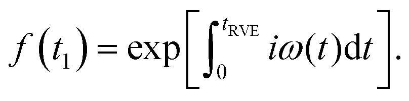 | (1) |
 | (2) |
The remaining simbols in this equation depict fundamental constants, such as vacuum permeability μ0, and g-values and electron or nuclear magnetons for A and B spins (gA,B, βA,B). To describe the time evolution in eqn (1), we introduce a sign factor s(t) of phase accumulation, which is chosen as +1 right after the primary (π/2)-pulse. This factor changes its sign at every refocusing (π)-pulse, and is zero during the RIDME mixing block, where the magnetization is along z and does not accumulate phase. For the refocused virtual echo we have s(t) = +1 for t < d1, s(t) = −1 for d1 < t < 2d1 + t1, s(t) = 0 for 2d1 + t1 < t < 2d1 + t1 + Tmix, s(t) = −1 for 2d1 + t1 + Tmix < t < 2d1 + d2 + Tmix, and s(t) = +1 for 2d1 + d2 + Tmix < t < 2d1 + 2d2 + Tmix. This is schematically shown in blue in Fig. 1. The refocusing condition  is fulfilled, meaning that phase accumulation due to both the resonance offset and the dipole–dipole coupling cancels. Furthermore, we have to analyze the case, when B-spins spontaneously flip at any time point t′ during the transverse evolution of the A spin. This is described by an additional factor h(t1,t) which starts at the value +1 at the beginning of the time evolution and changes its sign each time, when the B spin flips. After these additions, eqn (1) changes to
 | (3) |
We need to consider only the contribution of ωd to ω, since the B-spin flips affect only the sign of this contribution and we have already shown that s(t) cancels all other contributions. The many-spin solution is obtained, if we multiply the contributions from all B spins:
 | (4) |
To describe the macroscopic ensemble, we have to average eqn (4) over all spatial positions of the B-spins (r and θ), as well as over all possible realizations of the h(t) processes:
 | (5) |
 becomes small quickly for λ < 1 and k > 1. In fact, for λ < 0.5 all probabilities for k = 3, 4,… can be neglected to a good approximation, and the cases with k = 2 can be considered as a ‘weak perturbation’. For example, at λ = 0.5 we have PB(0) ≈ 0.606, PB(1) ≈ 0.303, PB(2) ≈ 0.076, and PB(3) ≈ 0.013. At λ = 0.2 we have PB(0) ≈ 0.819, PB(1) ≈ 0.164, PB(2) ≈ 0.016, and PB(3) ≈ 0.001.
Second, we assume for the moment that during the first Hahn echo block of duration 2d1, which is much shorter than T1,B in most cases, no B-spin flips occur. Thus, we only consider B-spin flips in the time period from the primary Hahn echo until the refocused virtual echo, which is used for detection of the RIDME signal. The consequence of including the first Hahn echo block into the calculations is discussed at the end of this section.
Let us first discuss the mixing block of length Tmix. We can compress the mixing block into a single point in the time evolution diagram (see Fig. 1), indicating that during this time s(t) = 0 and that no dipolar phase accumulation takes place. If the B spin flips an odd number of times during the mixing time Tmix, this corresponds to the inversion of the sign of the dipolar frequency. The probability of an odd number of flips can be computed as:42
 | (6) |
In eqn (6) the flip rate W has to be related to the longitudinal relaxation time as T1,B = 1/2W. If the number of B-spin flips is even, then no sign change for the dipolar frequency occurs. The probability of such an event is equal to
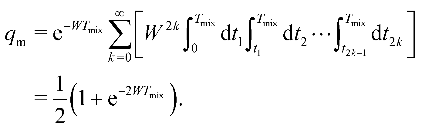 | (7) |
Additionally, let the probability be q when no B-spin flips occur during the transverse evolution time, and the probability be p when one B-spin flip occurs during this time. We can approximately write that p = λ/(1 + λ) and q = 1/(1 + λ).
Thus, we need to consider four different cases. Case 1 corresponds to the situation when no B-spin flips occur during the transverse evolution of A spins, and an even number of B-spin flips occurs during the mixing time Tmix. The probability of this event is P1 = q·qm. Case 2 corresponds to no B-spin flips during the transverse evolution of A spins, and an odd number of B-spin flips during the mixing time. The probability of this event is P2 = q·pm. Case 3 has one B-spin flip during the transverse evolution time, and an even number of B-spin flips during the mixing block, with P3 = p·qm, and, finally, case 4 has one B-spin flip during the transverse evolution and an odd number of B-spin flips during the mixing block, with the probability P4 = p·pm.
We now compute the absolute values of the trajectory integrals of the form
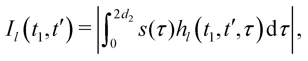 | (8) |
 | (9) |
The integration, according to eqn (9), results in the following correspondences: Ī1 = 0, Ī2 = 2t1, Ī3 = d2, and Ī4 = d2(1 − 2t1/d2 + 2t12/d22). Let us now return to the derivation of the RIDME background function F(t1). We can assume that every B spin has the same homogeneous spatial probability distribution, and the same relative probabilities for the four different cases of the stochastic evolution hl(t). We can, thus, rewrite the function F(t1) for a large number N of B spins as a product of N single-pair space-time averages of an identical form:
 | (10) |
Since the very large number of B spins is considered, we can conclude that, according to the central limit theorem, the average number Nl of the A–B pairs evolving according to the case l would be equal to Nl = PlN, and the fluctuations around these numbers will be statistically very small. We can thus rewrite eqn (10) in the form
 | (11) |
Each individual term Fl(t1) can be rewritten as:
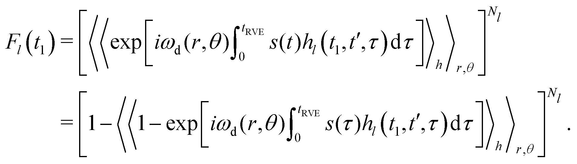 | (12) |
In the original work,42 Hu and Hartmann demonstrated that spatial averaging results in

Using our previously derived results for the time evolution averaging (eqn (9)), we can, thus, write for each case Fl(t1)

| Fl(t1) = exp[−Δω1/2PlĪl]. | (13) |
Here we used the abbreviation
 | (14) |
 | (15) |
We can now write explicitly all exponential terms
 | (16) |
 | (17) |
They can be separated into terms, which depend on the time t1, where the mixing block starts,
 | (18) |
 | (19) |
If we assume d2 ≪ T1,B, then for the non-varying factor F0 we arrive at the same equation as for the two-pulse echo decay in the original work of Hu and Hartmann: F0 = F2p(d2) = exp(−Δω1/2d22/T1,B).
We finally arrive at a compact representation of the RIDME background contribution due to spectral diffusion in the A–B spin system, which can be written as follows:
F(t1) = F0![[thin space (1/6-em)]](https://www.rsc.org/images/entities/char_2009.gif) exp[−Δω1/2(αt1 + βt12)]. exp[−Δω1/2(αt1 + βt12)]. | (20) |
The value Δω1/2 is defined above, and the factors α and β are defined as
 | (21) |
 | (22) |
If we consider the case of a DEER experiment in the presence of random flips of the B spins, the derivation of the background function F(t) would be similar. However, the pump pulse in DEER is rather short in time and we can neglect any spontaneous B-spin flips during the pump pulse. The inversion probability of the pump pulse λp would in this case substitute the probability of the odd number of B-spin flips during the RIDME mixing block. If we substitute in the above equations pm by λp and qm by 1 − λp, we, thus, obtain the equation for the background shape in the DEER case. This equation would, however, neglect the instantaneous diffusion due to the microwave pulses at the detection frequency. The combined action of the instantaneous and spectral diffusion was considered for the cases of some standard pulse sequences.43 For the RIDME background signal, it is feasible to assume that spectral diffusion is the major factor.
Eqn (20)–(22) allow us to discuss some general properties of the RIDME background function: first, both linear and quadratic terms in the exponent scale in the same way upon increasing the ratio Tmix/T1,B. When Tmix ≪ T1,B, the α and β coefficients are small, and depend approximately linearly on Tmix. They monotonically grow with increasing Tmix and reach limiting values α∞ = (T1,B − d2)/(T1,B + d2) and β∞ = 1/(T1,B + d2), when Tmix ≫ T1,B. Second, the coefficients α and β depend in different ways on d2 and T1,B. When d2 increases for given values of Tmix and T1,B, both α and β decrease, and the relative magnitude of the linear term in the exponent gets weaker as compared to the quadratic term. As a consequence, changing the length of the measured RIDME trace affects the shape of the background function. As we discuss in the following sections, this effect is, indeed, experimentally observed in regimes when T1 and Tm times of the paramagnetic species differ by less than an order of magnitude. If we reduce T1,B, for example, by increasing the measurement temperature, with constant values of Tmix/T1,B and d2, then the linear-term coefficient α decreases, while the quadratic-term coefficient β increases. Third, both the linear and the quadratic term in the exponent are proportional to the concentration of the paramagnetic species via the factor Δω1/2. Fourth, the quadratic terms in the exponent appear only in case 4, when B-spin flips occur both during the mixing block and during the transverse evolution of the A spins. When 2d2 ≪ T1,B, the RIDME background decay in the present model turns almost perfectly exponential.
It is worth mentioning once again that these equations are rather accurate only up to the value d2 = T1,B/2. The apparent problem that the term T1,B − d2 becomes negative at d2 > T1,B is then of no concern, since this happens outside of the validity range. At such lengths of the RIDME experiment, more than a single B-spin flip needs to be considered during the transverse evolution of A spins, and, thus, the equations need to be modified. For the complexes studied in this work, at a temperature of 30 K and, for long traces, even sometimes at 20 K, our assumptions do not always hold (see Table S2 in the ESI†).
The above calculations can be extended to the case of the full 5-pulse RIDME experiment, which would then include the dependency on the first interpulse delay of the primary echo block, d1. The derivation is lengthier than that detailed here, due to more possible spin–flip pathways. However, the final result has the same form as eqn (19)–(22), namely,
 | (23) |
| F5p(t1) = F5p,0exp[−Δω1/2(α5pt1 + β5pt12)], | (24) |
 | (25) |
 | (26) |
Importantly, the relative contribution of the mono-exponential versus the Gaussian decay is larger for longer d1 at the same d2. Of course, since we assume zero or one B-spin flip during the transverse evolution time 2(d1 + d2), the ratio (d1 + d2)/T1,B must be small and, accordingly, the mentioned effect must be weak. If the value d1 in eqn (25) and (26) increases with all other parameters being constant, then the coefficient α5p stays unchanged, neglecting contributions which scale with the power law (d1/T1,B)2 or higher. At the same time, the coefficient β5p decreases, thus making the overall decay of the RIDME background function slower. This is counterintuitive, but results from compensation between the average phase acquisition in the d1 and d2 intervals.
Mono-exponential longitudinal relaxation of B spins is a rather strong simplification that we used here to derive the analytic equations. In practice, in frozen glassy solvent mixtures, one observes distributions of T1 times, which are rather well described by stretched exponential decay functions. We, thus, can speculate that the real RIDME background shape will also be similar to a stretched exponential, and the stretching parameter will decrease when we change the experimental conditions in favor of the linear term, while it will increase, when we favor the quadratic term in eqn (20) and (24).
In the case of high-spin B species, such as Gd(III)27,28,44 or Mn(II)30,31,35 ions, the number of possible random trajectories for h(t) would be yet larger, since at each B-spin flip the dipolar frequency might change by one, two, or more units of ωd. However, the combination of linear and quadratic terms in the exponent would stay on, and the qualitative trends with respect to the changes of the critical parameters Tmix, d2 and T1,B would be the same.
Note that the derived equations also hold true, for instance, for the nuclear spin-induced spectral diffusion contribution to the RIDME background function. There could also be situations, when both electron and nuclear B spins play an important role in the RIDME background. In such cases, one also has to consider “interference contributions” when the flip during the transverse evolution time is due to one type of B spins, while the flip during the mixing block is due to another B-spin type. In particular, for describing such contributions, one would need to treat the situation with two unequal Δω1/2 values of the electron and the nuclear spin flip events, which can have similar strength since, for instance, the lower magnetic moment of the protons can be compensated by their large concentrations in H2O–glycerol mixtures. Note further that the RIDME background equations would also be applicable to the case of pairs of paramagnetic centers “slow spin”–“fast spin”, with non-identical A and B spins, which might have relaxation times differing by orders of magnitude.
3. Experimental and analysis details
3.1. Sample preparation
The background decay behaviour was studied with Gd(III), Mn(II), and Cu(II) complexes formed with the ligand MOMethynyl–PyMTA as well as on a single mutant (Q388C) of the cysteine-free RNA recognition motifs 34 (RRM34) of the polypyrimidine tract binding protein labeled with Gd–DOTA. The syntheses of Gd–PyMTA and Mn–PyMTA are described in ref. 30, 45 and 46. The synthesis of Cu–PyMTA is given in the ESI.† The compound solutions were filled into 0.5 mm i.d./0.9 mm o.d. quartz capillaries for W-band and 3 mm o.d. quartz capillaries for Q-band measurements, respectively. The samples were subsequently shock-frozen by immersion into liquid nitrogen before insertion into the precooled microwave cavity. For metal-ion–PyMTA stock solutions in D2O were diluted to final concentrations in the range of 25 to 500 μM, either with a 1:1 (v:v) D2O/glycerol-d8 or 1:1 (v:v) H2O/glycerol mixture. Protein expression and purification is described in ref. 47. The RRM34 mutant Q388C was labeled with Gd-maleimide–DOTA according to ref. 48. 550 μM stock solutions in a low salt buffer (10 mM NaPO4, 20 mM NaCl, pH = 6.5) were diluted 1:10 (v:v) in either D2O or H2O. Both solutions were then diluted 1:1 (v:v) in glycerol-d8.
3.2. EPR measurements
W band EPR experiments were performed using a commercial Bruker Elexsys E680 X/W band spectrometer as well as using a modified Bruker Elexsys E680 W band spectrometer,49–51 both operating at about 94 GHz. For the latter spectrometer, a home-built ENDOR cavity with a microwave frequency bandwidth of 130 MHz was used.49 The commercial spectrometer was equipped with a Bruker TE011 resonator. Q-band data were acquired using a Bruker Elexsys E580 Q band spectrometer equipped with a home-built cavity operating at about 34.5 GHz.18,52 A helium flow cryostat (ER 4118 CF, Oxford Instruments) was used to adjust the measurement temperature to 10, 20 or 30 K.Echo-detected (ED) field-swept EPR spectra were acquired using a Hahn-echo pulse sequence tp − τ − 2tp − τ with a pulse length tp of 12 ns. The interpulse delay τ was set to 400 ns. The power to obtain the π/2 − π pulses was set at the central transition of the Gd(III) spectrum by nutation experiments. Longitudinal relaxation measurements were performed using an inversion recovery sequence tinv − T − tp − τ − 2tp, in which the delay T was incremented starting from 1 μs. tinv = 12 or 16 ns and tp = 60 ns. Stimulated echo decays were recorded using tp − τ − tp − T − tp − τ for different τ values, increased T and tp = 12 ns. RIDME data were acquired using the refocused five pulse sequence shown in Fig. 1 with (π/2)-pulses being set to 12 ns and (π)-pulses to 24 ns. If not explicitly mentioned, the first interpulse delay was set to d1 = 400 ns and the starting point of the mixing block was set to t1,0 = −120 ns (120 ns before the first Hahn echo), while d2 was adjusted to the required trace length. The mixing time Tmix was varied to study its influence on the signal evolution, and it is specified in each case in the Results and Discussion section. To remove echo crossings and phase offsets, an eight-step phase cycle was used.26 For Q-band measurements, averaging of ESEEM contributions according to ref. 29 was performed.
3.3. Data analysis
Data were analyzed and processed with home-written MATLAB (The MathWorks Inc., Natick, MA, USA) scripts. In order to extract longitudinal relaxation times T1, inverted and offset corrected inversion-recovery traces were fitted by stretched exponential functions of the form c·exp(−(t/T1)x) using a nonlinear least-square fitting criterion based on the function ‘nlinfit’ (nonlinear regression) in MATLAB. Errors were extracted from the 95% confidence intervals of the fits using the function ‘nlparci’ (nonlinear regression parameter confidence intervals). Hahn-echo decay traces were processed by removing a constant offset averaged over the last 20 data points. The data were then fitted by stretched exponential functions of the form c·exp(−(t/Tm)x). Errors were extracted from the 95% confidence intervals of the fits.RIDME traces were fitted by a stretched exponential function (SE model) of the form c·exp(−(kt)d/3), a sum of two stretched exponential functions (SSE model) of the form ca·exp(−(kat)da/3) + cb·exp(−(kbt)db/3) or a product of two stretched exponential functions (PSE model) of the form c·exp(−(kat)da/3)·exp(−(kbt)db/3). If not stated explicitly the SE model was used. Fits were performed with MATLAB scripts, based on the functions ‘lsqcurvefit’ (nonlinear least-squares solver) and ‘nlparci’ (nonlinear regression parameter confidence intervals) from the Optimization and Statistic Toolbox. Similar to the DEER experiment, k quantifies the density of spins or decay rate and d is the dimensionality of the fitted function or stretching exponent. d = 3 corresponds to a mono-exponential function and d = 6 corresponds to a Gaussian decay function. Errors were estimated from the 95% confidence of the fit. An additional uncertainty was taken into account by varying the starting positions of the fit from 0 to about 200 ns after the zero time point as the region around the zero time point is in some cases distorted by an echo-crossing artefact. Note, however, that the MATLAB function mentioned above computes the confidence interval based on an approximate method, using the gradients at the best-fit point. This approach was found to provide good error estimates once the RIDME background trace was decayed to about 30–40% of the initial echo signal. For traces decaying only to about 60%, the errors were estimated manually (see the ESI† for details). The actual relative errors for d were about 10%. For traces decaying by only 10% of the initial value, the error was around 30%, depending in all these cases also on the particular signal-to-noise ratio, which was slightly varying between data sets. The corresponding relative errors for k were systematically smaller than for d. The inaccuracies allowed us only to discuss trends in d variations for the sample with 500 μM Gd–PyMTA concentration and for some of the data at 100 μM concentration. The much larger changes in k upon variation of temperature and concentration ensured that all trends observed for k were exceeding the estimated error bars. More details can be found in the Results and discussion section and in the ESI.†
4. Results and discussion
4.1. Transverse and longitudinal relaxation in Gd–PyMTA
Fig. 2 shows the transverse and longitudinal relaxation traces measured for Gd–PyMTA in a frozen, glassy D2O/glycerol-d8 matrix in the W band. We observed a strong temperature dependence of the Gd(III) electronic relaxation times T1 and Tm in the investigated temperature range from 10 to 30 K. Transverse relaxation times increase approximately by a factor of two for each temperature decrease of 10 K (see Fig. 2(a)). Longitudinal relaxation measurements (see Fig. 2(d)) exhibit a yet steeper increase of T1 with decreasing temperature. Longitudinal relaxation of the Gd–PyMTA centers is almost unaffected by a change in metal ion concentration from 25 to 500 μM (Fig. 2(e)) and only slightly affected for different detection positions within the EPR spectrum of Gd(III) (see Fig. 2(f)). In contrast, the transverse relaxation rate is significantly increased when the detection is moved away from the central peak in the Gd(III) spectrum (Fig. 2(c)). This phenomenon is related to differences in transverse relaxation of the different Gd(III) electronic transitions, which was previously discussed by Raitsimring et al.,53 and attributed to a ZFS-driven relaxation pathway. Here, however, we are most interested in the relaxation properties at the central peak of the Gd(III) spectrum, since this is the usual detection field position in the RIDME experiment. The field-dependent relaxation properties of high-spin metal centers are an interesting and important topic in itself, which deserves a dedicated study. | ||
| Fig. 2 Transverse (a–c) and longitudinal (d–f) relaxation traces for Gd–PyMTA (1:1 (v:v) D2O:glycerol-d8 matrix) in the W band. The T(1/e) times in the panels (a and d) report the times when the decay down to the 1/e level of the initial value is reached. (a and d) Temperature dependence at 25 μM, detection at the magnetic field position of the maximum EPR signal intensity, Bmax; (b and e) concentration dependence at 20 K, detection at Bmax; (c and f) dependence of the detection field position at 20 K and 100 μM. | ||
The characteristic transverse relaxation time of Gd(III) centers defines the upper limit of the detectable distance range in RIDME experiments. This might still be shortened if the RIDME background decay is too steep. The latter possibility is discussed in the following section. Here we conclude that the transverse evolution for the Gd–PyMTA complex in a deuterated matrix and at a low concentration (25 μM) allows detecting spin echoes after about 80 μs of transverse evolution, which corresponds to a distance of about 14 nm.54 Note that in this work we used protonated PyMTA and the intramolecular interactions between the electron and the proton spins would still make an additional contribution to the electronic relaxation.55
There is a clear concentration dependence of the shape of the transverse evolution decay for Gd–PyMTA. In a deuterated matrix, where the contribution by the electron–nuclear relaxation pathway is relatively weak, there is still a significant difference between the transverse relaxation curves measured at 100 μM and at 25 μM Gd–PyMTA concentration (Fig. 2(b)). Interestingly, while the characteristic 1/e decay time does not change significantly between these two concentrations, the shape of the Hahn echo decay curve clearly changes from a more mono-exponential-like shape for the 25 μM sample to a more bell-like shape for the 100 μM sample. This is a clear indication that the main relaxation mechanisms, contributing to the Hahn echo decay, change within this concentration range. It is likely that at 25 μM Gd–PyMTA concentration nuclear–electron spectral diffusion (NSD) along with ZFS-driven processes dominates the transverse relaxation, while at a concentration of 100 μM electron–electron spectral diffusion (ESD) starts to play a significant role.
Neither transverse nor longitudinal relaxation traces of Gd–PyMTA can be accurately fitted to mono-exponential functions. Most experimental data can be well approximated by stretched exponential functions. However, under some conditions the use of a sum of two stretched exponential functions resulted in a further improvement in the fit quality. A similar situation was observed earlier for nitroxide radicals and related to differences in intramolecular- and solvent-driven relaxation pathways.55 In the present case, this finding might be attributed to the diversity of the local surrounding in the glassy matrix, as well as to the presence of several relaxation pathways. We thus conclude that in frozen glassy solutions, the relaxation data need to be described by a distribution of Tm and T1 times. Consequently, distributions of the mono-exponential and the Gaussian decay rates are expected in the spectral diffusion processes during the RIDME experiment. Therefore, stretched exponential shapes are expected for the RIDME background decay, being either of more mono-exponential or more Gaussian character depending on the weighting of the pre-factors α and β in eqn (24). Based on the strong change in the transverse relaxation rate (Fig. 2(b)), we assume that, at 500 μM Gd–PyMTA concentration, the ESD processes dominate.
4.2. Stimulated echo decays of Gd–PyMTA
Compared to inversion recovery traces, stimulated echo decay is more sensitive to spectral diffusion and this sensitivity increases with an increase of the first interpulse delay τ due to a narrower spacing 1/τ (on the angular frequency scale) of the polarization grating with increasing τ.The W-band stimulated echo decay data for Gd–PyMTA in a deuterated water/glycerol frozen glassy matrix are shown in Fig. 3. A single homogeneous Markovian process is predicted to produce a mono-exponential dependence on the second delay time T in stimulated echo experiments.40 The experimental decay shapes are close to stretched-exponential functions and indicate that the assumption of a single homogeneous Markovian process is not sufficient for describing the data. If we consider electron–electron or electron–nuclear dipolar interactions, the width of the distribution of possible effective fields at the spatial point of an A spin is comparable to the strength of a single A–B spin coupling for several B spins which are in the nearest vicinity (among all B spins) of the A spin. Thus, a single B-spin flip might bring the resonance position of the A spin to the other side of the resonance frequency range, over which it can diffuse. Furthermore, the probability of frequency jumps in one or the other direction would correlate with the current resonance frequency of the A spin. For the A spins with effective field at the edges of this distribution and for the A spins with the effective field in the middle of the distribution the probabilities of the corresponding spontaneous increase and decrease of the effective field would not be the same. This breaks Markov's assumption that the probability distribution is independent of the pre-history of the stochastic process. Fortunately, the calculation routine used in this work allows avoiding this Markovian assumption, and thus is adequate for the description of the present case of spectral diffusion.
 | ||
| Fig. 3 W-band stimulated echo decay of Gd–PyMTA for different interpulse delays τ at different temperatures. Two concentration regimes were probed in a deuterated water/glycerol frozen glassy matrix: (a–c) 25 μM sample, negligible electron–electron coupling and (d–f) 500 μM, significant electron–electron interactions. (a and d) 10 K; (b and e) 20 K; (c and f) 30 K. | ||
In the absence of spectral diffusion, the stimulated echo decay still contains contributions from the longitudinal relaxation of the electron spins, since the second delay time is varied during the experiment. From the comparison of the data in the three lower panels of Fig. 2 with the data shown in Fig. 3, we conclude that the stimulated echo decay is faster than the longitudinal relaxation decay at all tested conditions. In line with the expectations, the characteristic decay time in the stimulated echo experiment gradually decreases with the increase of τ. The more pronounced change of characteristic decay time with τ for the sample containing 500 μM Gd–PyMTA, as compared to the sample with the 25 μM concentration, can be attributed to either a higher rate of spectral diffusion or a larger average strength of dipolar interactions for the more concentrated sample. To remove the contributions from longitudinal relaxation, constant time measurements, sensitive to spectral diffusion, would be useful. This approach can be realized with the 5-pulse version of the RIDME experiment, where the total times of transverse and longitudinal relaxation are identical for all measurement points.
4.3. Intermolecular background decay in refocused RIDME experiments with Gd–PyMTA
Relations of the relaxation times of the Gd(III)–PyMTA complexes to the delay settings in the refocused RIDME experiment are given in the ESI.†Fig. 4 shows the five-pulse RIDME background decay data for the Gd–PyMTA complex in frozen deuterated water/glycerol mixtures, as well as a comparison of the characteristic decay time between samples in protonated and deuterated solvents. Fig. 4(a) shows the dependence of the RIDME background decay on the concentration of the Gd(III) centers. The RIDME experiment is very sensitive to spectral diffusion driven mechanisms. Therefore, the changes in decay shape with spin concentration are more systematic than for the transverse relaxation traces in Fig. 2. One can clearly recognize a further increase of the characteristic decay time with decreasing concentration even between the samples with 100 μM and 50 μM Gd–PyMTA concentration.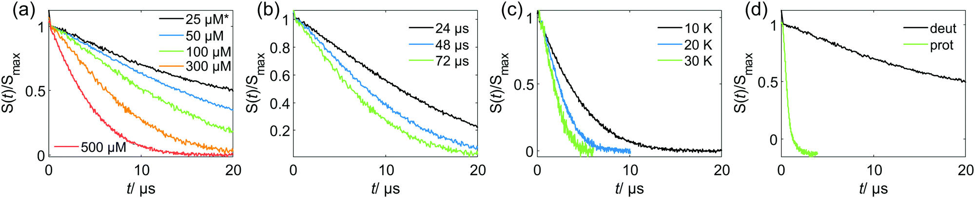 | ||
| Fig. 4 Experimental RIDME background decay of the Gd–PyMTA samples in the W band: (a) at 10 K, Tmix = 72 μs* and varying spin probe concentrations in deuterated solvent; *the 25 μM sample has Tmix = 96 μs (b) 300 μM spin probe concentration in deuterated solvent, at 10 K and varying Tmix; (c) 500 μM spin probe concentration in deuterated solvent, Tmix = 72 μs and varying measurement temperatures; (d) 25 μM spin probe concentration in deuterated or protonated solvent, at 10 K and Tmix = 96 μs. Note that the measurements are scaled to maximum intensity excluding the zero-time artefact. | ||
Fig. 4(b) shows the decrease of the characteristic decay time of the RIDME background trace with increasing mixing time, which well reproduces the trend predicted by eqn (21), (22), (25) and (26). Conceptually similar and, thus, leading to the same trend, is the decrease of the characteristic decay time with increasing measurement temperature, as shown in Fig. 4(c). An increase in temperature induces shorter T1,B times, and thus the ratio Tmix/T1,B increases at a constant mixing time.
Fig. 4(d) shows a comparison of the RIDME decay for a 25 μM Gd–PyMTA sample in protonated and deuterated water/glycerol. First, note that there is a further increase of the characteristic decay time in the deuterated sample at 25 μM as compared to that at 50 μM as shown in Fig. 4(a). This shows that even at the 50 μM electron spin concentration an electron-driven RIDME decay pathway plays an important role in deuterated solvents. Second, the comparison of the characteristic decay time reveals a drastic change if protons are replaced by deuterium. The coupling of the electron spin to the nuclear spin bath results in rapidly fluctuating environments at the electron spin site. These fluctuations, caused by nuclear spin diffusion, are much more efficient for proton than deuteron spins due to two reasons: (i) a proton spin flip corresponds to a stronger field change at the electron due to the larger magnetic moment of the proton, (ii) proton spin flips occur more frequently, since nuclear spin diffusion results from the coupling between the nuclear spins, which is much stronger for protons than for deuterons. The comparison reveals that the performance of the RIDME technique can be drastically improved by matrix deuteration.
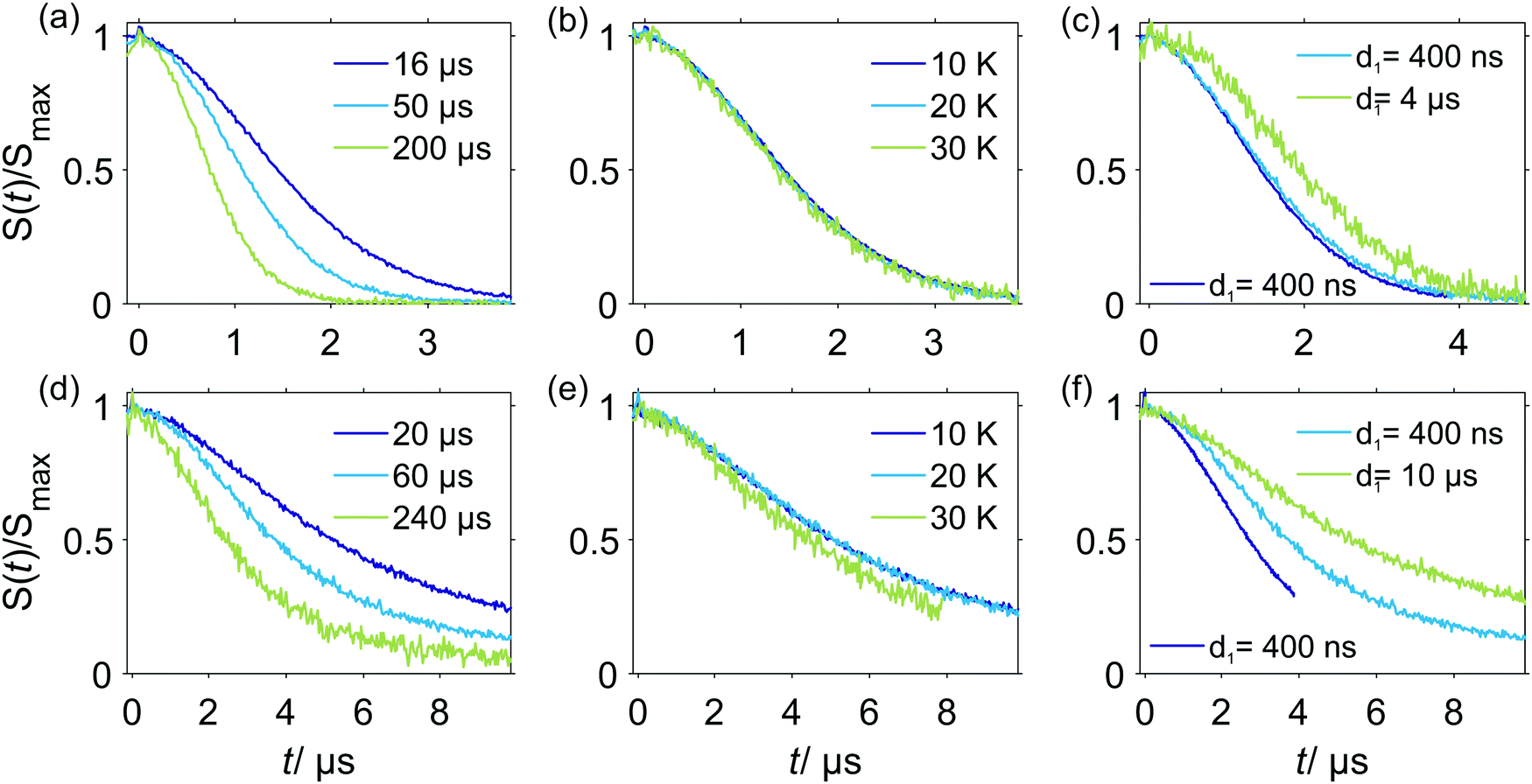
Eqn (21), (22) (25) and (26) predict a slower RIDME background decay for longer delays d1 and d2. This was, indeed, observed experimentally, as shown in Fig. 5. Fig. 5(a and b) show the trend of the decelerated background decay with an increasing delay d1, while Fig. 5(c) shows the effect for increasing the delay d2. Fig. 5(d) shows the effect for a simultaneous increase of d1 and d2. Note that in some series shown in Fig. 4, it was not possible to always keep the same delay time d2, e.g. for different Gd(III) concentrations or mixing times. The changes in the RIDME background decay times with Gd(III) concentration, mixing time or temperature, shown in Fig. 4 are, however, much larger than the changes with delay time variations in Fig. 5, thus making our previous discussions of the trends still valid. For instance, in Fig. 4(a) the change of the characteristic decay time between the 300 μM and 500 μM samples is larger than 50%, and the length difference in the RIDME background decay traces is about 20%. To compare, a still smaller change of the characteristic decay time is obtained if the length of the RIDME trace is increased more than three times from 3.2 μs to 10.2 μs, with all other experimental parameters kept constant (Fig. 5(c and d)).
 | ||
| Fig. 5 Experimental W-band RIDME background decays at 10 K for different interpulse delays (Tmix = T1, 100 μM Gd–PyMTA, 1:1 (v:v) D2O:glycerol-d8). (a) d2 = 3.2 μs, d1 = 400 ns and d1 ≈ d2; (b) d2 = 10.2 μs, d1 = 400 ns and d1 ≈ d2; (c) d1 = 400 ns, d2 = 3.2 and d2 = 10.2 μs; (d) d1 ≈ d2, d2 = 3.2 and d2 = 10.2 μs. Note that time traces are scaled to maximum intensity excluding the zero-time artefact. | ||
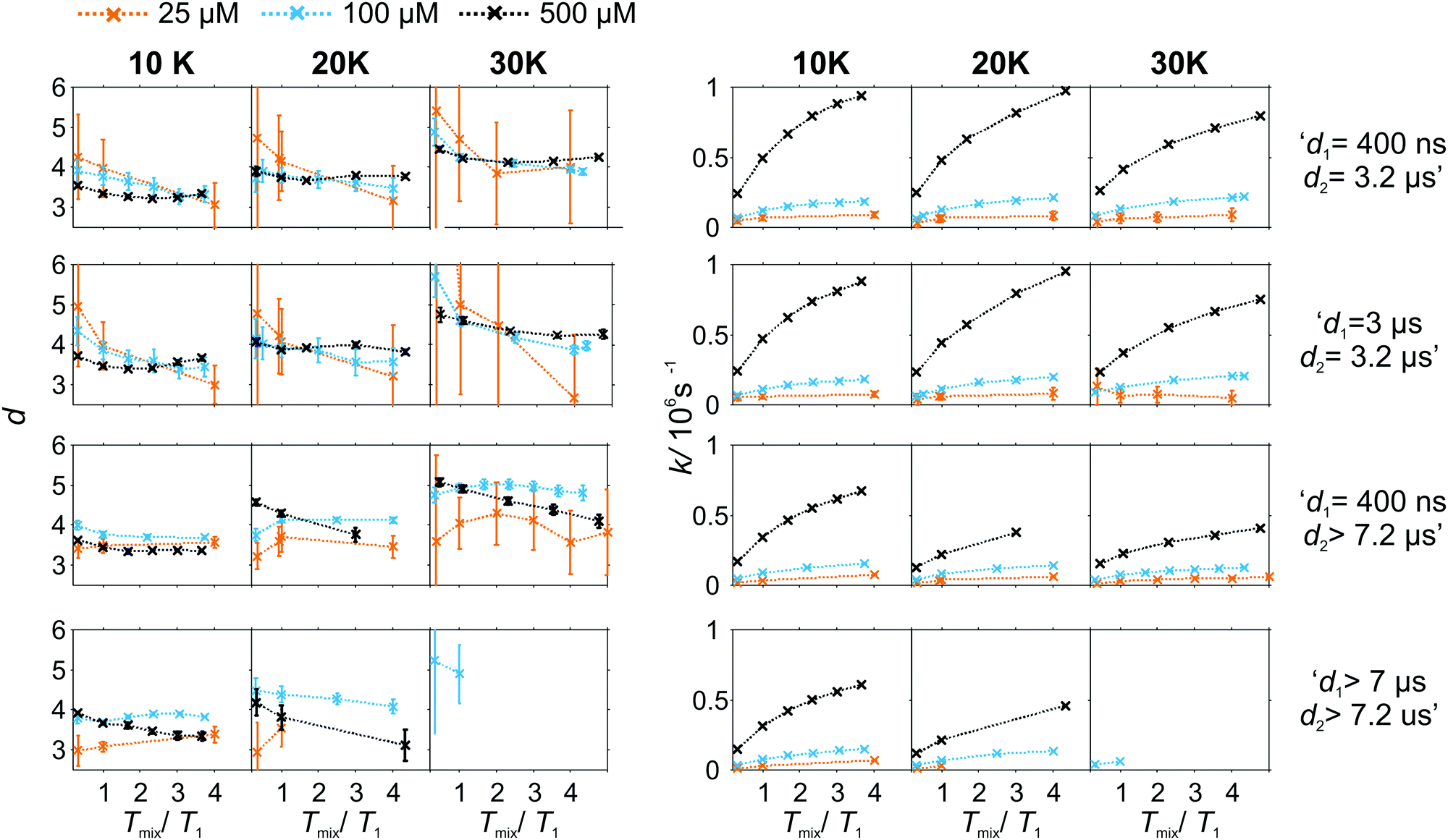
As the pulse sequence settings strongly influence the RIDME background decay, a systematic study of the influence of metal ion concentrations (25, 100, and 500 μM), measurement temperatures (10, 20, and 30 K) as well as mixing time periods was performed at four fixed pulse sequence settings. The trends obtained from fitting the refocused RIDME background decays with a single stretched exponential decay model to this set of data are illustrated in Fig. 6–8. Fig. 6 shows the dependencies of the dimensionality parameter d and decay rate constant k on the normalized mixing time Tmix/T1 for three Gd–PyMTA concentrations. The comparison in each panel is shown for one of the three temperatures: 10 K, 20 K or 30 K (left to right), and for one fixed set of delay times (d1, d2). Fig. 7, in turn, shows analogous graphs, comparing in each panel data for the listed three temperatures, while keeping the same Gd–PyMTA concentration, and fixed set of delay times (d1, d2). Finally, Fig. 8 compares the data for the four different time delay sets (d1, d2), with each panel dedicated to one fixed concentration and one fixed temperature. Fig. S6 and S7 (ESI†) show decay rates k with enlarged vertical axis to better visualize the differences in addition to Fig. 7 and 8, respectively.
 | ||
| Fig. 6 Comparison of the stretched exponent factor d and decay rate constant k versus the relative mixing time Tmix/T1 obtained from the analysis of experimental W-band RIDME decays at given pulse sequence settings (top to bottom) and measurement temperatures (left to right). The Gd–PyMTA concentration ranges are color encoded: orange 25 μM, light blue 100 μM, and purple 500 μM in 1:1 (v:v) D2O:glycerol-d8. | ||
 | ||
| Fig. 7 Comparison of the stretched exponent factor d and decay rate constant k versus the relative mixing time Tmix/T1 obtained from the analysis of experimental W-band RIDME decays in the deuterated solvent matrix at given pulse sequence settings (top to bottom) and spin concentration (left to right). The measurement temperature is color encoded: blue 10 K, green 20 K, and yellow 30 K. | ||
 | ||
| Fig. 8 Comparison of the stretched exponent factor d and decay rate constant k versus the relative mixing time Tmix/T1 obtained from the analysis of experimental W-band RIDME decays in the deuterated solvent matrix at the given measurement temperature (top to bottom) and spin concentration (left to right). The pulse sequence settings are color encoded: purple line (ss): d1 = 0.4 μs, d2 = 3.2 μs; dark blue line (ls): d1 = 3 μs, d2 = 3.2 μs; light blue line (sl): d1 = 0.4 μs, d2 = 10.2 μs and green line (ll): d1 = 10 μs, d2 = 10.2 μs. At 30 K, the long d2 value was only set to 7.2 μs and correspondingly d1 to 7 μs. At 20 K the green line (lm) corresponds to d1 = 7 μs and d2 = 7.2 μs and the yellow line (sm) to d1 = 0.4 μs and d2 = 7.2 μs. Cross marks correspond to a short interpulse daly d1 of 400 ns and circles to a long d1 on the order of d2. | ||
In general, for varying experimental conditions, accurate determination of the trends for the dimensionality parameter d was more difficult than for the decay constant k, because the relative changes in k were significantly larger. An accurate determination of d and k requires acquisition of RIDME traces, which are longer than the 1/k time (for a stretched exponential function this is equal to the 1/e time), and this was not always possible in a series of measurements with fixed sequence settings. Nevertheless, for short RIDME traces the product k·d can be determined rather accurately from the initial slope of the trace. Variations of the d parameter fall into the range between 3 and 6, corresponding to the expected range between the monoexponential and Gaussian decay. A slower decay of the RIDME traces at low Gd–PyMTA concentrations makes the determination of d values less accurate than for the highest tested Gd–PyMTA concentration. Similarly, at the same concentration the d values determined for shorter RIDME traces (shorter delay times d2) are less accurate than for longer ones due the shortened fitting range. Furthermore, at 30 K, where the relaxation times of Gd(III) centers are the shortest among the tested conditions, the signal-to-noise ratio is rather low. Thus, a higher inaccuracy of the fitted parameters is induced at 30 K as compared to those at 10 K and 20 K. The relative changes of k are much larger and, therefore, trends for the k parameter can be also determined from the measurements with short RIDME traces.
Eqn (21), (22), (25) and (26) predict no change of the dimensionality parameter for varying mixing times. In the experiment, however, we deal with distributions of transverse and longitudinal relaxation times, and the changes may result from a lower contribution of fast-relaxing species at long mixing times. For instance, in some panels, especially for high Gd–PyMTA concentrations and long transverse evolution delay times, there is a trend of decreasing d with increasing mixing time (see, for instance, in Fig. 7 the d dependence on Tmix/T1 in the two panels for 500 μM and long d2 and long or short d1). The scenario requires that the longitudinal relaxation time T1,A of A spins correlates with the longitudinal relaxation time T1,B of B spins in the near vicinity of the given A spin. This might happen, for example if the sample contains regions with slightly better and slightly worse glass quality. In such a sample, if the relaxation time of the A spin is slower than the average value through the whole sample, then the B-spins around this A spin will also relax slower than the average. The distribution of the relaxation times for such a sub-ensemble of B-spins would be narrower than the overall distribution, describing the entire sample. If such areas in the glass would not exist, then the distribution of the relaxation times of B spins around any A spin would be the same.
Another contribution might stem from the combined action of different types of B-spins (e.g. once nuclear spins and once electron spins) during the transverse evolution time and the mixing block. This can lead to interference effects of a more Gaussian or more exponential-like RIDME background decay shape. The weighting of both contributions would in such cases depends on the length of the mixing time. One might speculate that such trends are sometimes present in the left set of panels in Fig. 7.
A clear and systematic trend for the d parameter can be seen for the 500 μM Gd–PyMTA sample upon temperature variation (Fig. 7). With the increase in the sample temperature the ratio (d1 + d2)/T1,B becomes smaller, which enhances the relative contribution of the quadratic term, as compared to the linear term in eqn (21), (22), (25) and (26). This trend is still visible for the 100 μM sample. It is, however, absent or within precision of the performed background measurements for the 25 μM sample, where the nuclear spectral diffusion plays a key role in the shape of the RIDME background decay. Apparently, the flip rates of nuclear spins are smaller than for Gd(III) electron spins, and also the nuclear spin flip rates change much slower with temperature in the given temperature range from 10 K to 30 K. Both these effects would lead to the reduction of the magnitude of the discussed change of d with temperature.
Spectral diffusion contributions to the RIDME background shape increase at longer mixing times Tmix. This is also expressed in eqn (24). The characteristic decay rate k must increase with the increase of the ratio Tmix/T1,B as well as with the increase of the concentration of the B spins, which is clearly visible in all three Fig. 6–8. The ratio Tmix/T1,B can be altered by either changing the mixing time, or the longitudinal relaxation of the B spins. The latter can be achieved by increasing the sample temperature, which should lead to shorter T1,B. In the studied temperature range (10–30 K), this only affects the cases of electron spin dominated mechanisms. For Tmix ≪ T1,B, k should monotonically increase, flattening to a plateau for Tmix ≫ T1,B as suggested by eqn (24)–(26). These findings are reproduced in the experiments (Fig. 6) at higher electron spin concentrations. In cases of dominating nuclear-spin mechanisms (25 μM spin concentration), there seems to be a rather large T1,nuclei as we observe an almost linearly increasing k in the studied range of Tmix.
Note that, in Fig. 6–8, we always normalize the mixing time to the electronic longitudinal relaxation time T1,e. This partially compensates for the effect of changing temperature, so that, for instance, the dependencies of k on normalized mixing time for the 100 μM and 500 μM samples are nearly perfectly identical for the 10 K and 20 K data. Deviations from this trend for the 500 μM sample at 30 K or for the longest sets of transverse delays might be partially due to filtering effects on the relaxation time distributions. Furthermore, at this temperature, the used transverse evolution times d1 > 7 μs or d2 > 7.2 μs are already in the regime in which they approach T1,B. This alters the algebraic factors ((T1,B − (d2 − d1))/(T1,B + d1 + d2) and 1/(T1,B + d1 + d2)) in the equations for α and β and it can also lead to deviations from the derived theory due to the sufficiently high probability of more than one B-spin flip during the transverse evolution.
The change of the RIDME background decay coefficients upon changing the delays d1 and d2, illustrated by comparison of the decay traces in Fig. 5, can be seen as systematic trends in Fig. 8. The clearest trend is visible for the 500 μM sample where any increase of either d1 or d2 leads to a smaller k, which is predicted by the dependence of the factors α (eqn (21) and (25)) and β (eqn (22) and (26)) on d1 and d2. In line with the derived equations, the change of the coefficients is stronger with d2 than that with d1. At lower temperatures the trend upon changing d2 becomes somewhat weaker due to the influence of the longitudinal relaxation times of the Gd(III) centers on the coefficients. While this trend can still be recognized for the sample with 100 μM Gd–PyMTA concentration, it is invisibly weak for the 25 μM sample. As discussed above, due to the lower accuracy of d determination, no systematic changes of the d parameter could be determined in the series of transverse delay times with the 25 μM sample.
For the 100 μM and 500 μM samples we observed that for longer dipolar evolution times d2 the background dimensionality d weakly increases. This supports our theory: looking into eqn (21) and (22) it can be seen that α decreases with a factor of (T1 − d2) faster than β, which favors a more Gaussian-like decay with a higher dimensionality of the stretching exponent for longer delays d2.
The situation is more complex for a change in the d1 value. The changes in d as well as k, predicted by theory, are much smaller upon changing d1 than changing d2. While with increasing d1, β is predicted to decrease (eqn (26)), and α at the same time remains approximately constant (eqn (25)). This means, that a lower stretched exponent parameter d would be expected for a longer d1 evolution. In our experimental data, we observe that this parameter, however, increases. The effect is reduced at longer mixing times. The longer first interpulse delay allows a large number of spin flips during the transverse evolution, which might then in some way favor a Gaussian decay shape, yet a mono-exponential decay is favored by the longer mixing block.
Moving the detection position away from the central line of the Gd(III) spectrum leads to an accelerated RIDME background decay by an increase of the decay rate k (see Fig. S4 and S5, ESI†). It is accompanied by a shift of the background dimensionality to a more mono-exponential decay. However, the effect is only observed at short dipolar evolution delays d2 = 3.2 μs < Tm,Bouter, where Tm,Bouter stands for the phase memory time of Gd(III) centers at the spectral positions outside of the central peak. For longer delays (d2 > Tm,Bouter) the effect becomes insignificant. We speculate that the increase of the decay rate is driven by a stronger contribution of ZFS-driven flip-flops at the outer transitions. At longer delays d2 > Tm,Bouter, spins with a strong contribution to the transverse relaxation from the ZFS-driven pathway might be already decayed and thus filtered out.
4.4. RIDME background decays of a Gd(III) spin-labeled protein sample
In experiments with spin-labeled biomolecules it is sometimes difficult to prepare fully deuterated samples (including both deuterated solvents and deuterated biomolecules). An often more realistic scenario is that the spin-labeled protein stems from expression in protonated media, and is not deuterated, while the buffer solution is fully or partially deuterated. In this case the RIDME background decay may be dominated by the proton-driven NSD mechanism already at higher spin label concentrations. The spin label concentration threshold in such cases will depend on the overall average proton concentration in the sample.In Fig. 9 a set of RIDME background decays is shown for the two-domain construct RRM34 of PTBP1 spin labeled with Gd(III)–DOTA at residue Q388C, where the native amino acid was substituted by cysteine. The three upper panels show data for a partially deuterated solvent matrix (≈50% protons) composed of protonated water and deuterated glycerol, while the lower three panels present the data for an almost fully deuterated solvent matrix (<5% protons).
 | ||
| Fig. 9 Experimental W-band RIDME background decays of RRM34 Q388C Gd(III)–DOTA (≈30 μM). (a–c) in H2O buffer:glycerol-d8; (d–f) in D2O buffer:glycerol-d8. (a and d) 10 K, varying Tmix, d1 = 400 ns; (b) Tmix = 16 μs, d1 = 400 ns, varying temperatures; (e) Tmix = 20 μs, d1 = 400 ns; (c) at 10 K, Tmix = 16 μs and varying pulse sequence settings: purple line: d1 = 400 ns, d2 = 4.2 μs; blue line: d1 = 400 ns, d2 = 5.2 μs; green line: d1 = 4.2 μs, d2 = 5.2 μs; (f) at 10 K, Tmix = 60 μs and varying pulse sequence settings: purple line: d1 = 400 ns, d2 = 4.2 μs; blue line: d1 = 400 ns, d2 = 10.2 μs; green line: d1 = 10 μs, d2 = 10.2 μs. Note that the time traces are scaled to maximum intensity excluding the zero-time artefact. | ||
Comparison of the data in Fig. 9(a and d) reveals that deuteration of the buffer solution significantly increases the characteristic decay time of the RIDME background (by a factor of two to four) and, thus, facilitates measurements of longer spin–spin distances in RIDME experiments. Still, the characteristic decay times in these measurements are significantly shorter than for those of Gd–PyMTA in a fully deuterated solvent mixture, which can be attributed to the protons in the protein. Importantly, for a fixed mixing time (Fig. 9(b and e)) no temperature dependence of the RIDME decay shape was observed, except at 30 K in almost fully deuterated buffer solution. The exception most likely results from a shorter length of the trace at 30 K, which was enforced by a low sensitivity due to fast transverse relaxation at 30 K. Thus, we conclude that the proton flip rates relevant in the RIDME experiment are constant over the studied temperature range, at least between 10 K and 20 K. This suggests that at these temperatures and the studied concentration the spectral diffusion mechanism is driven by coupling of the electron spin to the surrounding bath, in which proton flips due to dipole–dipole couplings are temperature independent. These findings are also in line with the very strong change of the NSD contribution, once the protons are substituted by deuterium nuclei.
It is important to note that under some conditions the RIDME background decay is not well fitted by a single stretched exponential function as shown in Fig. 10(a). It follows from eqn (24) that the decay function is composed of a product of mono-exponential and Gaussian components. Taking into account the distribution of relaxation times, one could construct a test function which is a product of two stretched exponential functions, with the expectation that one of the two fitted d parameters will appear to be closer to three and the other one – closer to six. However, also fitting the protein RIDME data to a product of two stretched exponential functions does not improve the fit quality, as shown in Fig. 10(b). On the other hand, the trace can be fitted by a single stretched exponential function if the data trace is cut (Fig. 10(c)) or by a sum of two stretched exponential functions (Fig. 10(d)). This can be explained by the assumption that the spin label relaxes in different surroundings, depending on the conformation of the tether between the paramagnetic moiety and the protein backbone. One type of spin label surrounding, corresponding to more compact tether conformations, would contain more protons from the protein and would be characterized by shorter phase memory times Tm. The local surroundings of the spin label with more stretched tether conformations would be strongly influenced by the solvent deuterons, and would have a longer Tm. Of course, here we talk about a distribution of surroundings and Tm times, rather than about two distinct well-defined spin label states. This is in line with the strong influence of the spatial arrangement and degree of protonation for phase memory times Tm described earlier for DEER experiments.54 The local environmental effects on the spin-label phase memory relaxation time Tm of protonated proteins in deuterated solvents were also found to introduce a dependence on the distance distribution P(r) and on the length of the dipolar evolution period T.56
 | ||
| Fig. 10 Comparison of the fitting range and fitted model for the W-band RIDME background decays at 10 K. Spin-labeled protein mutant RRM34 Q388C in D2O buffer:glycerol-d8. (a) Stretched exponential function fit to full trace; (b) product of two stretched exponential function fit to full trace; (c) stretched exponential function fit to the first part of the trace; (d) sum of two stretched exponential functions fit to full trace. Note that the time traces are scaled to maximum intensity excluding the zero-time artefact. | ||
4.5. General discussion
The theoretical model, presented in this work, includes only one type of slowly flipping B spin with a defined flip rate. The analysis of the experimental RIDME data on frozen solutions of Gd–PyMTA and peptide-bound Gd–DOTA reveals that this simple model is capable of describing the key trends in the shape of the RIDME background decays. Experimental features can be understood using a combination of the presented theoretical model and the assumption of distributed relaxation times for A and B spins. The model predicts a mixture of mono-exponential and Gaussian decay curves for the RIDME background. From analysis of the experimental data we always obtained dimensionality parameters d between 3 (corresponding to the mono-exponential decay) and 6 (corresponding to the Gaussian decay). This is consistent with the theoretical prediction, provided we average the derived theoretical equations over a distribution of T1,B times. We see, however, in Fig. 11 that a product of the Gaussian and mono-exponential decay allows a slight improvement of the fits for an almost fully decayed trace. Yet, in many cases the systematic study presented above did not allow us to measure almost fully decayed traces, which makes the analysis more ambiguous and often no significant difference in the fit quality could be observed (see Fig. S2 and S3, ESI†) so that a single stretched exponential model was used for data analysis. | ||
| Fig. 11 W-band RIDME background decay curve and corresponding fits for 500 μM Gd–PyMTA in 1:1 (v:v) D2O:glycerol-d8 at 10 K with Tmix = 72 μs: (a) single stretched exponential function and (b) product of two stretched exponential functions. Note that the measurement are scaled to maximum intensity excluding the zero-time artefact. | ||
There are some weak trends in the d value, which seem to go above the estimated error bars, and for which some realistic speculations can be constructed based on the assumptions of distributed relaxation times, interference of the spin flips of different types of spins and, eventually, the distribution of the local glass quality throughout the EPR sample. The theoretical model presented here is also helpful in analyzing these scenarios. However, these effects are relatively weak as compared to the main trends for d and k.
Importantly, since the overall derivation scheme will not change in the presence of multiple relaxation pathways, for example due to the multi-level high-spin centers or due to several types of B spins, the theoretical model also allows discussing general trends in these, more complicated cases. The trends in the shape of the RIDME background data with respect to variation of different parameters are summarized in Table 1. Note that we observe weak trends for the changes in the transverse delay settings and much stronger trends with changing mixing time, temperature or concentration. These magnitudes of change are fully consistent with the equations derived above.
By far less exhaustive background measurements on Cu(II) or Mn(II) compounds do support the findings for the d and k parameters described in this section (for details see the ESI†). The transverse relaxation data in combination with the RIDME background data for the 25 μM Gd–PyMTA-complex in deuterated solvent suggest that Gd(III)–Gd(III) RIDME experiments with dipolar evolution periods up to 50 μs should be feasible (see Fig. 2(b) and 4(d)). The time of 50 μs corresponds to a decay of the Hahn echo to the 10% level of its initial intensity. For the d2 delay in RIDME experiment set to 50 μs we recorded RIDME background at 25 μM Gd(III) concentration and mixing time of 16 μs. According to the fits with a single stretched exponential function (SE) and a sum of two stretched exponential functions (SSE) the RIDME background signal was extrapolated to decay down to 40% of the initial signal intensity at the proposed maximal time of 50 μs. This time corresponds to one full period of dipolar oscillation for a spin–spin distance of approximately 13.5 nm. This distance can be thus taken for now as a rough estimate of the upper detectable distances for Gd(III)–Gd(III) RIDME, until direct experimental evidence is provided. Note, however, that fitting the background shape for such long dipolar evolution times might become difficult due to several decay contributions stemming from differential relaxation if no clear oscillations can be observed. One might consider using reference background measurements in such demanding situations to improve the overall quality of the background correction procedure. Note that if we compare the RIDME background shapes for the Gd(III) samples in fully protonated and fully deuterated solvent (Fig. 4(d)), we find that the change of the characteristic decay time between protonated and deuterated solvent cases exceeds the change in the gyromagnetic ratio between protons and deuterons. This implies that the nature of the nuclear contribution to the RIDME background might be more complicated than just a series of single spin flips. This phenomenon deserves a dedicated study.
For RIDME measurements in orthogonal pairs consisting of one organic radical and one metal center a typical situation would be that the RIDME background shape is mostly determined by the concentration and spatial distribution of the metal centers, because the longitudinal relaxation times of organic radicals are as a rule significantly longer than those of metal centers. The contribution from organic radicals might, however, become more significant if, for instance, their longitudinal relaxation rates are enhanced due to the presence of metal centers. In cases of unequal concentration of metal centers and organic radicals combined effects of longitudinal relaxation rates and spin concentrations have to be considered, in order to determine if the contributions from any type of paramagnetic species would dominate in the RIDME background shape. Such situations might appear, for instance, in studies of weak interactions between differently spin-labeled biomolecules, where one type of biomolecules needs to be present in excess.
RIDME measurements in biological samples are characterized by the presence of non-homogeneous proton distributions around the spin labels due to the use of deuterated solvents. On the one hand, this complicates the analysis of the intramolecular label-to-label distance distributions, since they are affected by the differences in the proton surrounding for different spin label tether conformations. On the other hand, the sensitivity of the RIDME background shape to the proton concentration can potentially be used as an auxiliary short- or middle-range constraint in biomolecular structure determination studies. It is difficult to define the actual sensitive distance range prior to a dedicated study. As a speculation we could propose that this should exceed the “pure NMR” range of the NOE-based constraints (i.e. r < 1 nm), and might appear to be comparable or even larger than the typical paramagnetic NMR distance range (between one and a few nanometers). Such a methodology, would, of course, first require detailed investigation of the proton-driven spectral diffusion mechanism, which appears to be more complicated than the electron-driven one. Such a study, which might be also relevant for low-temperature dynamic nuclear polarization (DNP), is currently underway in our lab.
Lastly, we would like to point out that some of the pathways considered here can be directly transferred to the case of a DEER experiment in pairs of non-equivalent A–B spins, with fast longitudinal relaxation of B spins. In such an experiment, when the length of the transverse evolution period starts to be comparable to the longitudinal relaxation time of B spins, the Gaussian decay contributions to the intermolecular DEER decay should appear in the same fashion as the quadratic term in eqn (24) appears due to a B spin flip during the transverse evolution time and one during the mixing block within one stochastic trajectory. Such contributions might be, for instance, present in Gd(III)–Gd(III) DEER, where a non-monoexponential background is often observed.57,58
5. Conclusions
In this work we provided a theoretical basis for describing the intermolecular RIDME background decay and discussed the most important practical aspects of intermolecular RIDME background measurements and their analysis. An important result of this work is the understanding that the RIDME background shape depends on all time delays in the RIDME pulse sequence and that the RIDME traces measured with different trace lengths need to be compared with care. This is particularly important for reference background measurements for biological applications, where exactly the same delay settings as in the original measurement need to be used in order to obtain the correct background decay shape.The applicability of the presented theoretical approach goes beyond the formal limitations of the simple A–B spin pair model analyzed in detail here, since more complicated spectral diffusion mechanisms can be described in very similar ways and would result in analogous trends for the RIDME background shape. The particular case of proton-driven electron spectral diffusion appears to be very interesting for elucidation of some steps in polarization transfer from electron spins to the nuclear spin bath. Such information would be valuable for improving low-temperature DNP techniques. Additionally, we propose that an understanding of the proton-driven spectral diffusion mechanism might help construct a RIDME-based approach to study the local or mid-range surrounding of spin labels attached to biomolecules.
Conflicts of interest
There are no conflicts of interest to declare.Acknowledgements
The work was supported by the Swiss National Science Foundation (grant 200020_169057) and by the Deutsche Forschungsgemeinschaft (DFG) within SPP 1601 (GO555/6-2). The authors thank Dr Michal Zalibera (Slovak University of Technology in Bratislava) for help with the primary RIDME measurements on Mn(II)–PyMTA, and for useful comments on the manuscript.References
- I. Krstic, B. Endeward, D. Margraf, A. Marko and T. F. Prisner, Structure and Dynamics of Nucleic Acids, Top. Curr. Chem., 2012, 321, 159–198 CrossRef CAS PubMed.
- O. Schiemann and T. F. Prisner, Long-range distance determinations in biomacromolecules by EPR spectroscopy, Q. Rev. Biophys., 2007, 40, 1–53 CrossRef CAS PubMed.
- G. Jeschke, DEER distance measurements on proteins, Annu. Rev. Phys. Chem., 2012, 63, 419–446 CrossRef CAS.
- G. Jeschke, Interpretation of Dipolar EPR Data in Terms of Protein Structure, Struct. Bonding, 2014, 152, 83–120 CrossRef.
- R. Igarashi, T. Sakai, H. Hara, T. Tenno, T. Tanaka, H. Tochio and M. Shirakawa, Distance Determination in Proteins inside Xenopus laevis Oocytes by Double Electron–Electron Resonance Experiments, J. Am. Chem. Soc., 2010, 132, 8228–8229 CrossRef CAS PubMed.
- I. Krstić, R. Hänsel, O. Romainczyk, J. W. Engels, V. Dötsch and T. F. Prisner, Long-Range Distance Measurements on Nucleic Acids in Cells by Pulsed EPR Spectroscopy, Angew. Chem., Int. Ed., 2011, 123, 5176–5180 CrossRef.
- M. Qi, A. Groß, G. Jeschke, A. Godt and M. Drescher, Gd(III)-PyMTA Label Is Suitable for In-Cell EPR, J. Am. Chem. Soc., 2014, 136, 15366–15378 CrossRef CAS PubMed.
- A. Martorana, G. Bellapadrona, A. Feintuch, E. Di Gregorio, S. Aime and D. Goldfarb, Probing Protein Conformation in Cells by EPR Distance Measurements using Gd3+ Spin Labeling, J. Am. Chem. Soc., 2014, 136, 13458–13465 CrossRef CAS PubMed.
- Z. Yang, Y. Liu, P. Borbat, J. L. Zweier, J. H. Freed and W. L. Hubbell, Pulsed ESR Dipolar Spectroscopy for Distance Measurements in Immobilized Spin Labeled Proteins in Liquid Solution, J. Am. Chem. Soc., 2012, 134, 9950–9952 CrossRef CAS PubMed.
- G. Y. Shevelev, O. A. Krumkacheva, A. A. Lomzov, A. A. Kuzhelev, O. Y. Rogozhnikova, D. V. Trukhin, T. I. Troitskaya, V. M. Tormyshev, M. V. Fedin, D. V. Pyshnyi and E. G. Bagryanskaya, Physiological-Temperature Distance Measurement in Nucleic Acid using Triarylmethyl-Based Spin Labels and Pulsed Dipolar EPR Spectroscopy, J. Am. Chem. Soc., 2014, 136, 9874–9877 CrossRef CAS PubMed.
- G. E. Fanucci and D. S. Cafiso, Recent advances and applications of site-directed spin labeling, Curr. Opin. Struct. Biol., 2006, 16, 644–653 CrossRef CAS PubMed.
- J. P. Klare and H.-J. Steinhoff, Spin labeling EPR, Photosynth. Res., 2009, 102, 377–390 CrossRef CAS PubMed.
- E. Bordignon, Site-directed spin labeling of membrane proteins, Top. Curr. Chem., 2012, 321, 121–157 CrossRef PubMed.
- W. L. Hubbell, C. J. Lopez, C. Altenbach and Z. Yang, Technological advances in site-directed spin labeling of proteins, Curr. Opin. Struct. Biol., 2013, 23, 725–733 CrossRef CAS.
- M. Pannier, S. Veit, A. Godt, G. Jeschke and H. Spiess, Dead-Time Free Measurement of Dipole–Dipole Interactions between Electron Spins, J. Magn. Reson., 2000, 142, 331–340 CrossRef CAS PubMed.
- G. Jeschke, A. Koch, U. Jonas and A. Godt, Direct conversion of EPR dipolar time evolution data to distance distributions, J. Magn. Reson., 2002, 155, 72–82 CrossRef CAS PubMed.
- G. Jeschke, G. Panek, A. Godt, A. Bender and H. Paulsen, Data analysis procedures for pulse ELDOR measurements of broad distance distributions, Appl. Magn. Reson., 2004, 26, 223–244 CrossRef CAS.
- Y. Polyhach, E. Bordignon, R. Tschaggelar, S. Gandra, A. Godt and G. Jeschke, High sensitivity and versatility of the DEER experiment on nitroxide radical pairs at Q-band frequencies, Phys. Chem. Chem. Phys., 2012, 14, 10762–10773 RSC.
- S. Saxena and J. H. Freed, Double quantum two-dimensional Fourier transform electron spin resonance: distance measurements, Chem. Phys. Lett., 1996, 251, 102–110 CrossRef CAS.
- P. P. Borbat and J. H. Freed, Multiple-quantum ESR and distance measurements, Chem. Phys. Lett., 1999, 313, 145–154 CrossRef CAS.
- G. Jeschke, M. Pannier, A. Godt and H. Spiess, Dipolar spectroscopy and spin alignment in electron paramagnetic resonance, Chem. Phys. Lett., 2000, 331, 243–252 CrossRef CAS.
- A. Doll, S. Pribitzer, R. Tschaggelar and G. Jeschke, Adiabatic and fast passage ultra-wideband inversion in pulsed EPR, J. Magn. Reson., 2013, 230, 27–39 CrossRef CAS PubMed.
- P. E. Spindler, S. J. Glaser, T. E. Skinner and T. F. Prisner, Broadband inversion PELDOR spectroscopy with partially adiabatic shaped pulses, Angew. Chem., Int. Ed., 2013, 52, 3425–3429 CrossRef CAS PubMed.
- A. Doll and G. Jeschke, Fourier-transform electron spin resonance with bandwidth-compensated chirp pulses, J. Magn. Reson., 2014, 246, 18–26 CrossRef CAS PubMed.
- L. Kulik, S. Dzuba, I. Grigoryev and Y. Tsvetkov, Electron dipole–dipole interaction in ESEEM of nitroxide biradicals, Chem. Phys. Lett., 2001, 343, 315–324 CrossRef CAS.
- S. Milikisyants, F. Scarpelli, M. G. Finiguerra, M. Ubbink and M. Huber, A pulsed EPR method to determine distances between paramagnetic centers with strong spectral anisotropy and radicals: The dead-time free RIDME sequence, J. Magn. Reson., 2009, 201, 48–56 CrossRef CAS PubMed.
- S. Razzaghi, M. Qi, A. I. Nalepa, A. Godt, G. Jeschke, A. Savitsky and M. Yulikov, RIDME Spectroscopy with Gd(III) Centers, J. Phys. Chem. Lett., 2014, 5, 3970–3975 CrossRef CAS PubMed.
- A. Collauto, V. Frydman, M. D. Lee, E. H. Abdelkader, A. Feintuch, J. D. Swarbrick, B. Graham, G. Otting and D. Goldfarb, RIDME distance measurements using Gd(III) tags with a narrow central transition, Phys. Chem. Chem. Phys., 2016, 18, 19037–19049 RSC.
- K. Keller, A. Doll, M. Qi, A. Godt, G. Jeschke and M. Yulikov, Averaging of nuclear modulation artefacts in RIDME experiments, J. Magn. Reson., 2016, 272, 108–113 CrossRef CAS PubMed.
- K. Keller, M. Zalibera, M. Qi, V. Koch, J. Wegner, H. Hintz, A. Godt, G. Jeschke, A. Savitsky and M. Yulikov, EPR characterization of Mn(II) complexes for distance determination with pulsed dipolar spectroscopy, Phys. Chem. Chem. Phys., 2016, 18, 25120–25135 RSC.
- D. Akhmetzyanov, H. Y. V. Ching, V. Denysenkov, P. Demay-Drouhard, H. C. Bertrand, L. C. Tabares, C. Policar, T. F. Prisner and S. Un, RIDME spectroscopy on high-spin Mn2+ centers, Phys. Chem. Chem. Phys., 2016, 18, 30857–30866 RSC.
- A. V. Astashkin, Mapping the Structure of Metalloproteins with RIDME, in Methods in enzymology, ed. P. Z. Qin and K. Warncke, Academic Press, 2015, ch. 10, vol. 563, pp. 251–284 Search PubMed.
- D. Abdullin, F. Duthie, A. Meyer, E. S. Muller, G. Hagelueken and O. Schiemann, Comparison of PELDOR and RIDME for Distance Measurements between Nitroxides and Low-Spin Fe(III) Ions, J. Phys. Chem. B, 2015, 119, 13534–13542 CrossRef CAS PubMed.
- A. Meyer, D. Abdullin, G. Schnakenburg and O. Schiemann, Single and double nitroxide labeled bis(terpyridine)-copper(II): influence of orientation selectivity and multispin effects on PELDOR and RIDME, Phys. Chem. Chem. Phys., 2016, 18, 9262–9271 RSC.
- A. Meyer and O. Schiemann, PELDOR and RIDME Measurements on a High-Spin Manganese(II) Bisnitroxide Model Complex, J. Phys. Chem. A, 2016, 120, 3463–3472 CrossRef CAS PubMed.
- A. Giannoulis, M. Oranges and B. E. Bode, Monitoring Complex Formation by Relaxation-Induced Pulse Electron Paramagnetic Resonance Distance Measurements, ChemPhysChem, 2017, 18, 2318–2321 CrossRef CAS PubMed.
- A. Giannoulis, C. L. Motion, M. Oranges, M. Bühl, G. M. Smith and B. E. Bode, Orientation selection in high-field RIDME and PELDOR experiments involving low-spin Co(II) ions, Phys. Chem. Chem. Phys., 2018, 20, 2151–2154 RSC.
- A. D. Milov, A. G. Maryasov and Y. D. Tsvetkov, Pulsed electron double resonance (peldor) and its applications in free-radicals research, Appl. Magn. Reson., 1998, 15, 107–143 CrossRef CAS.
- A. M. Portis, Spectral diffusion in magnetic resonance, Phys. Rev., 1956, 104, 584–588 CrossRef CAS.
- J. R. Klauder and P. W. Anderson, Spectral diffusion decay in spin resonance experiments, Phys. Rev., 1962, 125, 912 CrossRef CAS.
- W. B. Mims, Phase Memory in Electron Spin Echoes, Lattice Relaxation Effects in CaWO4:Er,Ce,Mn, Phys. Rev., 1968, 168, 370–389 CrossRef CAS.
- P. Hu and S. R. Hartmann, Theory of spectral diffusion decay using an uncorrelated-sudden-jump model, Phys. Rev. B: Solid State, 1974, 9, 1–13 CrossRef.
- K. M. Salikhov, S. A. Dzuba and A. M. Raitsimring, The theory of electron spin-echo signal decay resulting from dipole-dipole interactions between paramagnetic centers in solids, J. Magn. Reson., 1981, 42, 255–276 CAS.
- K. Keller, V. Mertens, M. Qi, A. I. Nalepa, A. Godt, A. Savitsky, G. Jeschke and M. Yulikov, Computing distance distributions from dipolar evolution data with overtones: RIDME spectroscopy with Gd(III)-based spin labels, Phys. Chem. Chem. Phys., 2017, 19, 17856–17876 RSC.
- M. Qi, M. Hülsmann and A. Godt, Synthesis and Hydrolysis of 4-Chloro-PyMTA and 4-Iodo-PyMTA Esters and Their Oxidative Degradation with Cu(I/II) and Oxygen, Synthesis, 2016, 3773–3784 CAS.
- J. A. Clayton, K. Keller, M. Qi, J. Wegner, V. Koch, H. Hintz, A. Godt, S. Han, G. Jeschke, M. S. Sherwin and M. Yulikov, Quantitative analysis of zero-field splitting parameter distributions in Gd(III) complexes, Phys. Chem. Chem. Phys., 2018, 20, 10470–10492 RSC.
- C. Gmeiner, D. Klose, E. Mileo, V. Belle, S. R. A. Marque, G. Dorn, F. H. T. Allain, B. Guigliarelli, G. Jeschke and M. Yulikov, Orthogonal Tyrosine and Cysteine Site-Directed Spin Labeling for Dipolar Pulse EPR Spectroscopy on Proteins, J. Phys. Chem. Lett., 2017, 8, 4852–4857 CrossRef CAS PubMed.
- C. Gmeiner, G. Dorn, F. H. T. Allain, G. Jeschke and M. Yulikov, Spin labelling for integrative structure modelling: a case study of the polypyrimidine–tract binding protein 1 domains in complexes with short RNAs, Phys. Chem. Chem. Phys., 2017, 19, 28360–28380 RSC.
- A. Nalepa, K. Mobius, W. Lubitz and A. Savitsky, High-field ELDOR-detected NMR study of a nitroxide radical in disordered solids: towards characterization of heterogeneity of microenvironments in spin-labeled systems, J. Magn. Reson., 2014, 242, 203–213 CrossRef CAS PubMed.
- N. Cox, W. Lubitz and A. Savitsky, W-band ELDOR-detected NMR (EDNMR) spectroscopy as a versatile technique for the characterisation of transition metal–ligand interactions, Mol. Phys., 2013, 111, 2788–2808 CrossRef CAS.
- L. Rapatskiy, N. Cox, A. Savitsky, W. M. Ames, J. Sander, M. M. Nowaczyk, M. Rogner, A. Boussac, F. Neese, J. Messinger and W. Lubitz, Detection of the water-binding sites of the oxygen-evolving complex of Photosystem II using W-band 17O electron-electron double resonance-detected NMR spectroscopy, J. Am. Chem. Soc., 2012, 134, 16619–16634 CrossRef CAS PubMed.
- R. Tschaggelar, B. Kasumaj, M. G. Santangelo, J. Forrer, P. Leger, H. Dube, F. Diederich, J. Harmer, R. Schuhmann, I. Garca-Rubio and G. Jeschke, Cryogenic 35 GHz pulse ENDOR probehead accommodating large sample sizes: Performance and applications, J. Magn. Reson., 2009, 200, 81–87 CrossRef CAS.
- A. Raitsimring, A. Dalaloyan, A. Collauto, A. Feintuch, T. Meade and D. Goldfarb, Zero field splitting fluctuations induced phase relaxation of Gd3+ in frozen solutions at cryogenic temperatures, J. Magn. Reson., 2014, 248, 71–80 CrossRef CAS.
- H. El Mkami and D. G. Norman, EPR Distance Measurements in Deuterated Proteins, in Methods in Enzymology, ed. P. Z. Qin and K. Warncke, Academic Press, 2015, ch. 5, vol. 564, pp. 125–152 Search PubMed.
- J. Soetbeer, M. Hülsmann, A. Godt, Y. Polyhach and G. Jeschke, Dynamical decoupling of nitroxides in o-terphenyl: a study of temperature, deuteration and concentration effects, Phys. Chem. Chem. Phys., 2018, 20, 1615–1628 RSC.
- J. L. Baber, J. M. Louis and G. M. Clore, Dependence of Distance Distributions Derived from Double Electron–Electron Resonance Pulsed EPR Spectroscopy on Pulse-Sequence Time, Angew. Chem., Int. Ed., 2015, 54, 5336–5339 CrossRef CAS.
- M. Yulikov, P. Lueders, M. F. Warsi, V. Chechik and G. Jeschke, Distance measurements in Au nanoparticles functionalized with nitroxide radicals and Gd3+-DTPA chelate complexes, Phys. Chem. Chem. Phys., 2012, 14, 10732–10746 RSC.
- A. Dalaloyan, M. Qi, S. Ruthstein, S. Vega, A. Godt, A. Feintuch and D. Goldfarb, Gd(III)–Gd(III) EPR distance measurements – the range of accessible distances and the impact of zero field splitting, Phys. Chem. Chem. Phys., 2015, 17, 18464–18476 RSC.
Footnote |
| † Electronic supplementary information (ESI) available. See DOI: 10.1039/c8cp07815g |
| This journal is © the Owner Societies 2019 |