 Open Access Article
 This Open Access Article is licensed under a
 Creative Commons Attribution 3.0 Unported Licence
A screening of results on the decay length in concentrated electrolytes†
Henrik
Jäger‡
 a,
Alexander
Schlaich‡
ab,
Jie
Yang
bc,
Cheng
Lian
c,
Svyatoslav
Kondrat
*bd and
Christian
Holm
*b
a,
Alexander
Schlaich‡
ab,
Jie
Yang
bc,
Cheng
Lian
c,
Svyatoslav
Kondrat
*bd and
Christian
Holm
*b
aStuttgart Center for Simulation Science (SC SimTech), University of Stuttgart, 70569 Stuttgart, Germany
bInstitute for Computational Physics, University of Stuttgart, Stuttgart, Germany. E-mail: svyatoslav.kondrat@gmail.com; skondrat@ichf.edu.pl; holm@icp.uni-stuttgart.de
cSchool of Chemistry and Molecular Engineering, East China University of Science and Technology, Shanghai 200237, China
dInstitute of Physical Chemistry, Polish Academy of Sciences, 01-224 Warsaw, Poland
First published on 21st August 2023
Abstract
Screening of electrostatic interactions in room-temperature ionic liquids and concentrated electrolytes has recently attracted much attention as surface force balance experiments have suggested the emergence of unanticipated anomalously large screening lengths at high ion concentrations. Termed underscreening, this effect was ascribed to the bulk properties of concentrated ionic systems. However, underscreening under experimentally relevant conditions is not predicted by classical theories and challenges our understanding of electrostatic correlations. Despite the enormous effort in performing large-scale simulations and new theoretical investigations, the origin of the anomalously long-range screening length remains elusive. This contribution briefly summarises the experimental, analytical and simulation results on ionic screening and the scaling behaviour of screening lengths. We then present an atomistic simulation approach that accounts for the solvent and ion exchange with a reservoir. We find that classical density functional theory (DFT) for concentrated electrolytes under confinement reproduces ion adsorption at charged interfaces surprisingly well. With DFT, we study confined electrolytes using implicit and explicit solvent models and the dependence on the solvent's dielectric properties. Our results demonstrate how the absence vs. presence of solvent particles and their discrete nature affect the short and long-range screening in concentrated ionic systems.
1 Introduction
Electrolytes and ionic liquids (ILs) are virtually everywhere. In biological systems, electrolytes and electrostatic interactions play a crucial role in nearly all processes, regulating the osmotic pressure and the body's water content,1,2 controlling enzymatic cascade reactions,3,4 transmitting nerve signals,5,6 contracting muscles,7–9etc. The role of ILs in industrial applications is also hard to overestimate.10,11 Ions and electrostatic interactions are essential in applications as diverse as capacitive energy storage12–14 and conversion,12,15 sensors,16 and catalysis.17,18Despite this broad applicability and extreme importance in fundamental life-sustaining processes, our understanding of ionic interactions, particularly ionic screening, is still incomplete. Ionic interactions are exponentially screened; this so-called Debye screening arises from a cloud of counter-ions surrounding each ion. Formally, it can be obtained using the linearised Poisson–Boltzmann equation, also known as the Debye–Hückel equation. The screening length resulting from this theory is known as the Debye screening length. For monovalent ions, it is given by eqn (1),
 | (1) |
This elegant and physically intuitive picture of an ionic screening cloud is, however, only valid for dilute electrolytes and breaks down as the ion density increases. The theory of screening in concentrated electrolytes was developed in the mid-1990s.19,20 While it does not provide a simple equation (like eqn (1)) for the screening length ξ, it predicts that ξ increases with ion density (ρ) above the so-called Kirkwood crossover,21 a crossover from the monotonic to oscillatory decay of the charge–charge correlation function. Note that the Debye length monotonically decreases with ρ.
Recent surface force balance (SFB) experiments22–24 have challenged our understanding of ionic correlations by reporting unusually large screening lengths, about an order of magnitude larger than predicted by classical theory. Ascribed to the bulk properties of ionic systems, such screening was termed25,26 ‘underscreening’ to stress that the interactions are ‘under-screened’ compared to what is expected from classical theories.19,20 More recent work27,28 named it ‘anomalous underscreening’ meaning that the screening predicted by classical theories already ‘under-screens’ the interactions compared to Debye screening. The experiments in ref. 22–24 have renewed research activities in the field of concentrated electrolytes. Although the origin of anomalous underscreening still needs to be revealed, a new wave of theoretical and simulation work has given us new insight, while also demonstrating gaps in our understanding of the behaviour of concentrated electrolytes.
In the first part of this contribution, we provide a brief overview of experimental studies on underscreening (Section 2.1), discuss classical theories of ionic screening (Section 2.2.1), and review more recent theoretical (Section 2.2.2) and simulation (Section 2.3) studies motivated by the underscreening experiments.22–24 As our overview shows, the main focus of the theoretical and simulation studies has been on ILs and dense electrolytes in bulk, while screening in confined systems and by ion–solvent mixtures received less attention. In Section 3, we use atomistic simulations and classical density functional (DFT) theory and attempt to fill this gap by studying how solvent and confinement affect the structure and screening in concentrated electrolytes.
2 Brief overview of previous results
2.1 Underscreening experiments
The first report on an unusually long screening length dates back to the last decade. In 2013, Gebbie et al.22 studied IL-mediated forces between crossed cylinders using SFB and a [C4mim]+[NTf2]− ionic liquid, followed by studies of several other ILs23 in 2015. From the long-range behaviour of the measured forces, these authors extracted screening lengths, ξ, that were about one order of magnitude larger than expected from classical theories.19,20,29 They explained these surprising results as ions forming neutral “ion pairs” leading to the Debye-like screening determined by a small fraction of “free” ions, an approach criticised by Perkin et al.30 and Lee et al.31By systematically analysing screening lengths in different concentrated electrolytes and room temperature ILs, Smith et al.24 found that “the electrostatic screening length in concentrated electrolytes increases with concentration”. While the increase is, in principle, in agreement with classical theories19,20,29 (cf. Fig. 2), the repeatedly measured large values of ξ were surprising and still remain a mystery.32 In follow-up work, Lee et al.25,26 revealed that all experimental data available at the time collapsed onto a single curve given by eqn (2),
| ξ/λD ∼ (σion/λD)n | (2) |
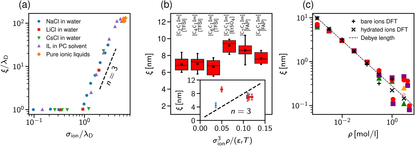 | ||
| Fig. 1 Ionic screening lengths from experiments. (a) Screening length divided by the Debye length λD plotted as a function of the ion diameter σion divided by λD. The symbols show experimental data for various ionic liquids and aqueous electrolytes collected from ref. 24–26. According to ref. 25 and 26, all values collapse onto a single curve displaying cubic scaling, eqn (2) with n = 3, for σion/λD ≳ 1. (b) Screening lengths of six ionic liquids from ref. 36. The inset shows the screening lengths as a function of σion3ρ/(εrT), which follows from eqn (2) with n = 3, demonstrating deviation from the cubic scaling. (c) Screening lengths vs. ion concentration from ref. 28. The filled symbols show atomic force microscopy (AFM) results for various electrolytes. The black dash line corresponds to the expected Debye length and the crosses and pluses to the DFT results (see Section 2.2.2) with hydrated and bare ion diameter, respectively. | ||
The authors of ref. 26 explained underscreening as the emergence of charged defects in an overall neutral, nearly crystalline IL. However, as noted by Adar et al.,35 this physical picture is only applicable at concentrations above ≈5 M, while the experiments show cubic scaling at much lower concentrations. To link underscreening to the bulk properties of electrolytes, Lee et al.25,26 related the large screening lengths to other experimentally measurable quantities, viz. excess chemical potential, μex, and differential capacitance, Cd. However, Zeman et al.33 criticised this relation by showing that ‘screening lengths’ extracted from the experimental data on μex and Cd using the models proposed in ref. 25 and 26 disagree with the screening lengths measured experimentally in ref. 22–24.
The experiments of ref. 22–24 have motivated several studies on other ILs and concentrated electrolytes using various experimental techniques. While most of the published studies support underscreening,37,38 there are also studies reporting either large ξ but no cubic scaling36 or no anomalously large screening lengths at all;28,39 examples are shown in Fig. 1b and c, respectively.
2.2 Theory
 | ||
| Fig. 2 Ionic screening lengths from classical theories. In both plots, the screening lengths are plotted as functions of the ion diameter divided by the Debye length λD. The largest screening length determines the asymptotic behaviour. The solid and dotted lines show the screening lengths due to electrostatic and hard-core domination, respectively. (a) Ornstein–Zernike equation and the hypernetted chain closure by Attard19 and (b) generalised mean spherical approximation by de Carvalho and Evans.20 | ||
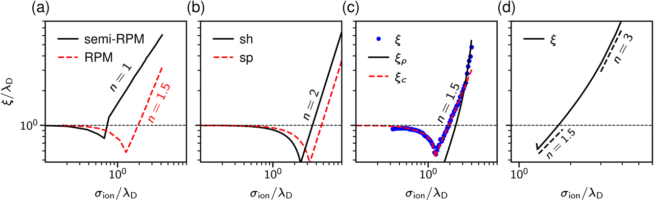 | ||
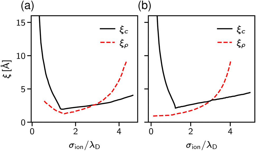
| Fig. 3 Theoretical predictions for ionic screening lengths. In all plots, the screening lengths are divided by the Debye length λD and plotted as a function of the ion diameter divided by λD. (a) Mean spherical approximation for an ionic liquid (black solid line), described by a restricted primitive (RPM) model, and an ionic liquid-solvent mixture (red dashed line), modelled as charged and neutral hard spheres (semi-RPM). Note the different scaling exponents n = 1 and n = 3/2. Data from ref. 40. (b) Extended mean field theory modified to account for ion sizes35 predicts a quadratic scaling (‘sh’ and ‘sp’ denote spherical shell and homogeneous sphere models for ions). (c) DFT results for the decay length of the solvation force compared to the decay lengths of the total and charge density profiles at a wall (ξρ and ξc). Data from ref. 34. (d) Results of the Ciach–Patsahan theory showing that exponent n changes continuously from n = 1.5 close to the Kirkwood point to n = 3 for 2.5 ≲ σion/λD ≲ 4. Note that the x-axis has a different range than the other panels. Data from ref. 41. | ||
Adar et al.35 calculated the charge–charge correlation function on the Gaussian level, but modified the Coulomb kernel to account for the excluded volume interactions between neighbouring ions. These authors considered two ion models: a homogeneously charged sphere and a homogeneously charged spherical shell. They found that, above the Kirkwood point, the decay length of the charge–charge correlation function increases with the concentration with the scaling exponent n = 2 for both models (Fig. 3b).
Cats et al.34 used DFT44–46 with various MSA-like approximations for the electrostatic interactions and fundamental measure theory (FMT)47–50 for hard core interactions to study charge and total density correlation functions of the RPM. Above the Kirkwood point, they found an increasing decay length dominated by electrostatics and the scaling exponent n = 1.5, which seems to be characteristic of the MSA for the primitive model.40 In line with Attard19 and de Carvalho and Evans,20 they saw a cross-over to the hard-core dominated screening as the concentration increased (Fig. 3c).
In contrast to previous work that reported scaling exponents n < 3, Ciach and Patsahan42,43 arrived at an exponent n = 3 using a self-consistent Gaussian approximation based on the Brazovskii approach.51,52 Unlike previous theoretical approaches, these authors took into account the local variance of the charge density. However, similar to the phenomenology of ref. 25 and 26, their theory appears to be valid only at unusually high concentrations (e.g., above ≈23 mol l−1 for aqueous sodium chloride and ≈5 mol l−1 for room temperature ILs taking bare ion diameters, see ref. 33). We recall that experimentally the cubic scaling was reported at much lower concentrations (≈1 mol l−1).
In more recent work, Ciach and Patsahan41 found that the exponent n is not constant but varies with σion/λD from n = 1.5 close to the Kirkwood point to n = 3 for 2.5 ≲ σion/λD ≲ 4, increasing further for σion/λD > 4 (Fig. 3d). These authors also found two other exponents n = 1 and n = 5, but for the density–density decay length.41
The cubic scaling in ref. 41–43 emerged in the dampened oscillatory decay of the charge–charge correlation function. In experiments, however, the force exhibiting large screening lengths with cubic scaling decayed monotonically with distance between the surfaces. Kjellander53,54 showed the possibility of long-range monotonic decay at high densities using dressed ion theory.55,56 However, to our knowledge, this approach is yet to be applied to experimental or simulation data of ionic systems with anomalously large screening lengths and cubic scaling.
2.3 Simulations
Studying underscreening with molecular simulations is challenging because huge boxes and long simulation runs must be considered to capture the possible appearance of the experimentally measured large screening lengths. Coles et al.57 studied aqueous LiCl and NaI, and lithium bis(trifluoromethane)sulfonimide [Li][TFSI] in water and an organic solvent mixture of dimethoxyethane and dioxolane. By analysing the charge–charge correlation functions, they found that the decay length increases with concentration, and reported a scaling exponent n ≈ 1.3 (Fig. 4a). We note, however, that these authors studied simulation systems with box lengths from about 9 nm to 11 nm. The monotonic underscreening decay was reported for separations between 4 and 7 nm for ILs (screening lengths from 2 nm to 10 nm) and up to 3 nm for aqueous NaCl (screening lengths from 1 nm to 3 nm).22–24 The simulated systems were, therefore, at the edge or even too small for the underscreening regime.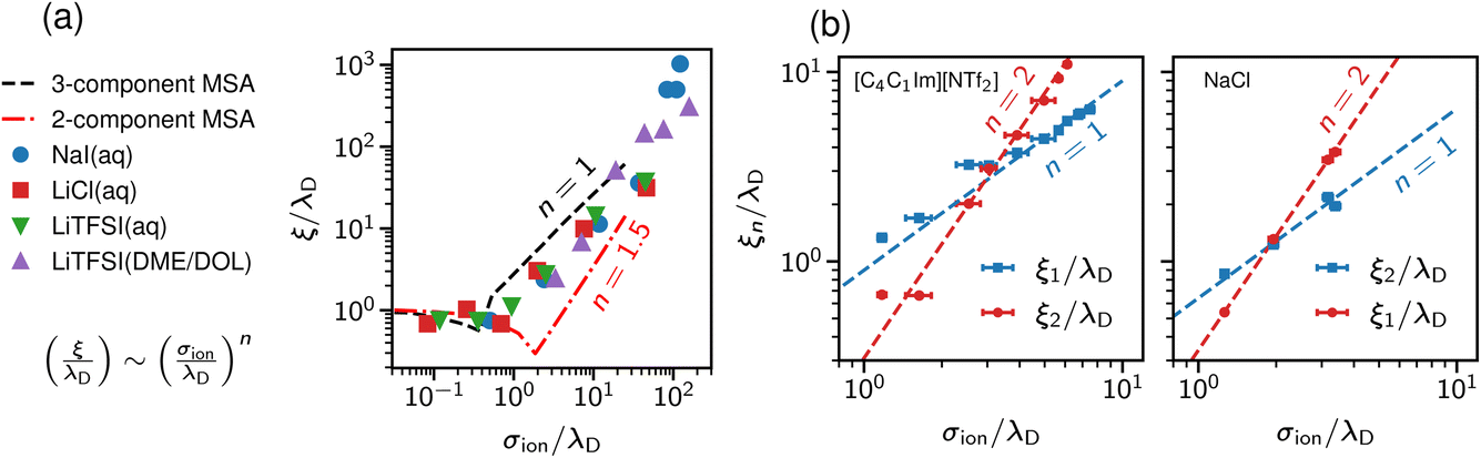 | ||
| Fig. 4 Screening lengths from molecular dynamics simulations. (a) Simulation results for a few ionic liquids and aqueous electrolytes obtained by Coles et al.57 MSA results are displayed for comparison. The MSA results are shown for the restricted primitive model (RPM) and the RPM with non-polar solvent of the same size as the ions. The simulation results show scaling given by eqn (2) with n ≈ 1.3. (b) Large-scale simulation results for 1-butyl-3-methylimidazolium bis(trifluoromethanesulfonyl)-imide ([C4C1Im][NTf2], left plot) and aqueous NaCl (right plot). Data from ref. 58. | ||
Zeman et al.33,58 studied aqueous NaCl with all-atom simulations and 1-butyl-3-methylimidazolium hexafluorophosphate ([C4C1Im] [PF6]) with both all-atom and coarse-grained simulations. They considered simulation box sizes from about 10 nm to 50 nm, depending on the system, to allow the evaluation of potentials of mean-force (PMF) at experimentally relevant distances. They did not find any sign of underscreening down to the accuracy of 10−5kBT in the PMF. Instead, they revealed a crossover between the scaling with exponent n = 1 and n = 2 (Fig. 4b). Zeman et al.33 also studied confined [C4C1Im] [PF6] and found that the screening lengths obtained from the density and electric field profiles are in good quantitative agreement with the bulk simulations.
The semi-primitive electrolyte model was considered with MD simulations by Coupette et al. Unlike classical theories (Fig. 2) and DFT calculations (Fig. 3c), which predict a crossover from the electrostatics to hard-core dominated screening regime (above the Kirkwood cross-over), they found a crossover in the reverse order, i.e., from the hard-core to an electrostatics dominated regime upon increasing ion concentration. In their most recent work, Härtel et al.27 studied the primitive electrolyte model and reported anomalously large screening lengths. However, these authors considered a strong coupling regime (large Bjerrum lengths), leading to the formation of ionic clusters even at low densities and Debye-like screening determined by ‘free’ ions. It remains to be seen if this picture stays valid in an experimentally relevant weak coupling regime.
3 How surfaces, confinement and solvent influence the ionic structure and screening
As we see from this brief overview, the main focus of theory and simulations has been on bulk ILs and electrolytes, motivated by the claim that underscreening is a bulk property of concentrated ionic systems. However, how and on which length scale does the presence of surfaces and confinement modify ionic screening? In simulations of confined fluids, one usually fixes the number of species (i.e., the number of solvent and salt molecules in the case of electrolytes) to the corresponding densities in bulk, which might differ considerably in confinement. These issues have been addressed for all-atom simulations only in the case of salt-free simulations (i.e., only counter-ions screening the surface charge and no salt) using for example grand-canonical Monte Carlo (GCMC) simulations60 or advanced free energy perturbation (FEP)61 to extrapolate to the bulk chemical potential,62 depending on the desired accuracy. For example, water GCMC simulations are known to converge slowly at an accuracy of ±1 solvent molecules,63 an issue which is even more complicated for complex ILs. In Section 3.1.1, we extend our previously established thermodynamic extrapolation approach to control the water chemical potential63–65 to a simultaneous extrapolation of the solvent and salt chemical potentials based on FEP and apply it to a confined electrolyte.Another question that previous studies have neglected is the effect of solvent. While solvent was present in some atomistic simulations,33,57,58 a systematic understanding of the role of solvent in electrostatic screening is still lacking. In theoretical approaches and coarse-grained simulations,40,59 solvent molecules were modelled as non-polar neutral hard spheres, while a constant relative dielectric permittivity, independent of the local ion and solvent density, described the dielectric properties of the solvent. But how does the structure of a polar solvent, which directly screens the ion–ion interactions, affect ionic screening? In this section, we first employ atomistic molecular simulations at a prescribed chemical potential to study how surface and confinement effects can modify the composition of an aqueous electrolyte (NaCl) confined between accurately modelled mica sheets (Fig. 5a). Density functional theory (DFT) calculations using an explicit solvent model (Fig. 5b) reveal systematic surface depletion of the salt and solvent density profiles that both agree remarkably well with MD simulations. We then use an implicit solvent model (Fig. 5c) to investigate the effect of spatially resolving solvent molecules on the ionic screening and the structure of confined ILs.
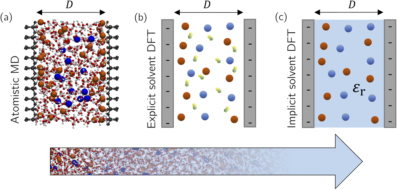 | ||
| Fig. 5 Modelling approaches ranging from atomistic simulations to implicit solvent DFT calculations. (a) Snapshot of the atomistic simulation system. Water (small red and white spheres show oxygen and hydrogen, respectively) together with the electrolyte ions (large orange and blue spheres show sodium and chloride, respectively) are confined between mica sheets separated by a distance D between the outermost mica atoms. Schematics of two charged plates confining an electrolyte with explicit (b) and implicit (c) solvent models. Cations and anions have the same diameter σion and solvent molecules consist of two oppositely charged beads of the same diameter σs. The plate separation is D in both models. | ||
3.1 Methods
As alluded, the natural choice of the ensemble for the simulation of a confined system is the grand-canonical ensemble, since ions and water molecules can be exchanged with a reservoir in the relevant experimental setups, thus balancing the chemical potentials of the system under investigation with an external reservoir. In practice, grand-canonical approaches for aqueous or IL systems suffer from major convergence problems.63 We build upon the thermodynamic extrapolation method64 to determine the correct composition of the confined system, viz. the Ns and Nion of solvent and salt species. The key idea is to determine the chemical potential of each species for different system compositions (Ns, Nion), see Section S1 in the ESI.† Thus, the multidimensional optimisation problem of the system composition corresponding to the chemical potentials (μs, μion) is transformed into independent relations of Nα(μα) at fixed concentration of all other species (see Fig. 6b). In practice, the inverse problem is solved, i.e., μα(Nα)|{Nβ}, determined at a fixed composition of all other species (β) to extrapolate the particle numbers that correspond to the desired chemical potential in bulk at a given salt concentration. The non-monotonic behaviour of the chemical potential of water observed in Fig. 6b in general makes the extrapolation difficult to apply. However, the chemical potential of the ion pairs is largely independent of the number of solvent molecules, i.e. the water chemical potential can be tuned once a suitable number of ion pairs has been chosen.
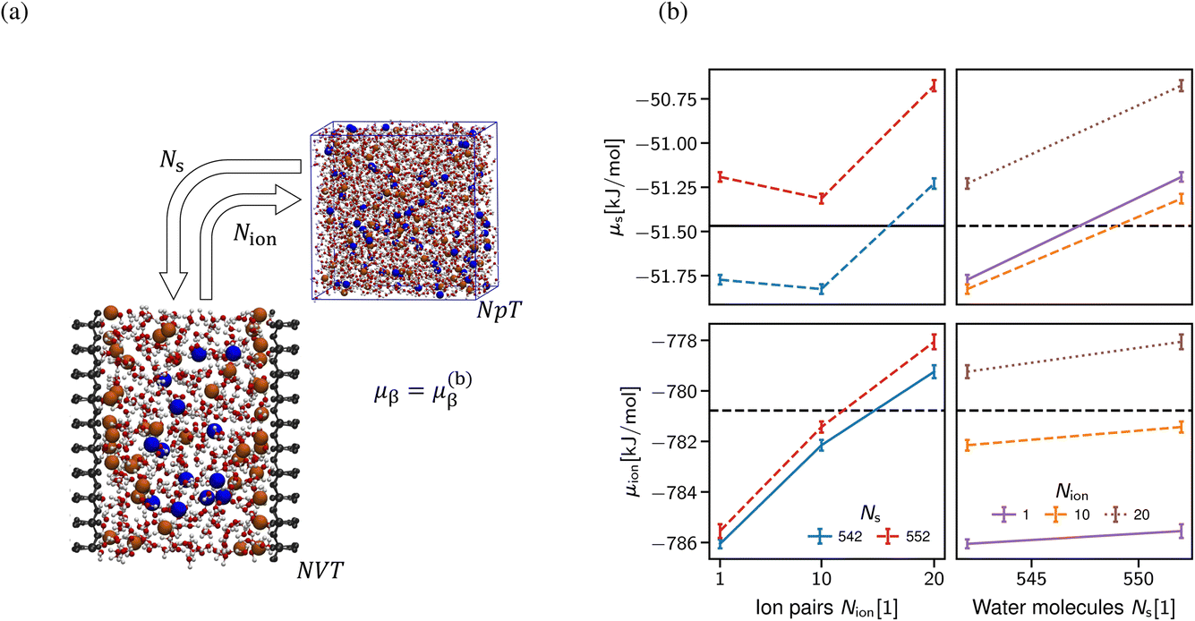 | ||
| Fig. 6 Extrapolation of the correct system composition. (a) The chemical potential of each species is calculated in the centre of the slit for a range of different system compositions (Ns, Nion). Since the numerical value of the chemical potential is highly dependent on the force field used, we use the reference potentials from molecular dynamics simulations of a bulk electrolyte at given salt concentrations as the baseline. (b) The multidimensional optimisation problem of system composition (Ns, Nion) and chemical potential (μs, μion) is broken down into independent minimisations in N and μ for each species, as illustrated here for 2 mol l−1. The ion species is largely unaffected by the number of solvent molecules, yet the chemical potential of the solvent species is highly affected by the number of ion pairs. To obtain a usable set of particle numbers, we choose them such that the chemical potential of both species is closest to the reference values corresponding to the desired concentration in the bulk. | ||
A clear disadvantage of this approach is its computational cost, since the uncertainty in the chemical potentials must be very small (in the order of 0.01 kBT) to reliably predict the composition as shown in Fig. 6b. This requires simulation times of >100 ns per FEP state (Section S1 in the ESI†), thus amounting to at least 5 μs for each data point shown in Fig. 6b. For this reason, we limit the application of this approach to only determine the correct composition of a single system size D = 2 nm, which then yields the desired chemical composition and thus allows for meaningful comparison with the classical DFT calculations shown in Section 3.2.1. Note that (i) the extraction of density oscillation decay lengths requires significantly larger simulation boxes58 and (ii) obtaining the pressure decay length requires a significant number of different slit sizes D.
The interaction potential between a pair of charged beads (either solvent or ions), i and j, separated by a distance r, is given by eqn (3),
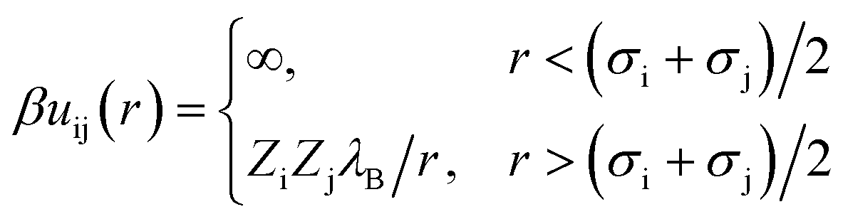 | (3) |
We consider the electrolyte confined between two positively charged walls with surface charge density Q = 0.5e nm−2. This slit pore with surface-to-surface separation D interacts with species i through the hard-wall potential, as in eqn (4),
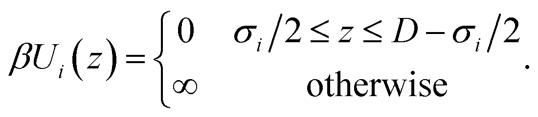 | (4) |
Note that the electric field inside the slit is zero, making the wall interaction in eqn (4) independent of the surface charge, which only enters via the charge neutrality condition.
Within DFT, the equilibrium density profiles are determined by minimising the grand potential, eqn (5),
 | (5) |
![[triple bond, length as m-dash]](https://www.rsc.org/images/entities/char_e002.gif) (rs+, rs−) denotes the two coordinates specifying the position of the two beads of the solvent dimer and Us(R) = Us+(rs+) + Us−(rs−).
(rs+, rs−) denotes the two coordinates specifying the position of the two beads of the solvent dimer and Us(R) = Us+(rs+) + Us−(rs−).
The total intrinsic Helmholtz free energy F consists of the ideal part and the excess contribution Fex, i.e.eqn (6),
 | (6) |
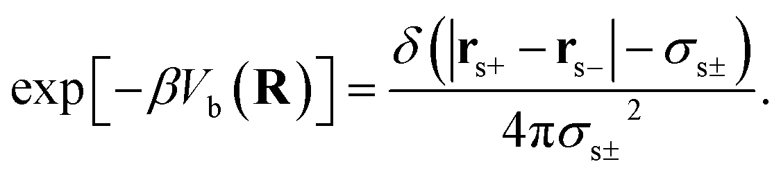
The first and second terms are only present in the case of explicit solvent, and Vb is the bonding potential of a (rigid) solvent molecule given by eqn (7)70
 | (7) |
The excess Helmholtz free energy Fex consists of different molecular interactions and correlations given by eqn (8)
| Fex = Fhsex + FCex + Felex + Fchex, | (8) |
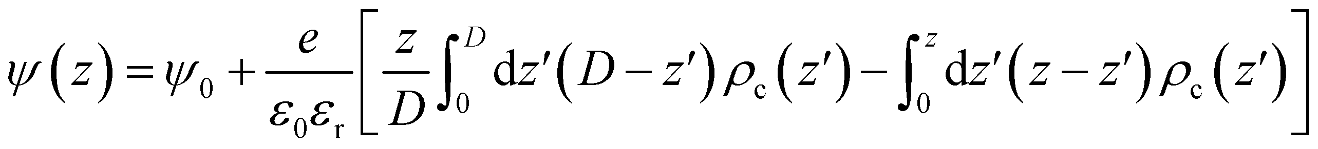
The Coulomb energy was directly obtained by integrating Poisson's equation, ∇2ψ(r) = ρc(r)/ε0εr, where ρc(r) is the local charge density and ψ(r) the local electrostatic potential. For the one-dimensional slab system and using ψ(z = 0) = ψ(z = D) = ψ0, we get eqn (9)
 | (9) |
We solved the Euler–Lagrange equations following from the minimisation of eqn (5) using the conventional Picard iteration method.75 We used the bulk concentrations as an initial guess for the density profiles to determine Fex and ψ(z) and performed iterations until a relative accuracy of 10−8 in densities at all positions was achieved. Convergence was obtained for discretisation Δz = (1−5) × 10−2σs depending on the salt concentration and plate separation. We ensured a constant surface charge density Q through appropriate choice of ψ0. The interaction pressure was then obtained by numerically differentiating eqn (5), i.e., P = −δ(Ω/A)δD, and the extrapolation of D → ∞ gave us the corresponding bulk pressures. We note that the bulk values differ for the implicit and explicit solvent models and amount to βσion3Pb ≈ 2.4 and ≈23, respectively.
3.2 Results
![[small rho, Greek, macron]](https://www.rsc.org/images/entities/i_char_e0d1.gif) α(z) = ρα(z)/ρα(b), obtained using our atomistic MD simulations in a mica slit pore of width D = 2 nm. Note that the z-axis is shifted with respect to the Gibbs dividing surface76 (GDS) of species j, zG(j), which follows from the surface excess of species i with respect to j, as described in eqn (10)
α(z) = ρα(z)/ρα(b), obtained using our atomistic MD simulations in a mica slit pore of width D = 2 nm. Note that the z-axis is shifted with respect to the Gibbs dividing surface76 (GDS) of species j, zG(j), which follows from the surface excess of species i with respect to j, as described in eqn (10)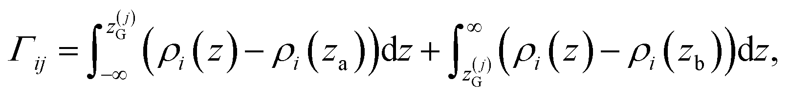 | (10) |
 | (11) |
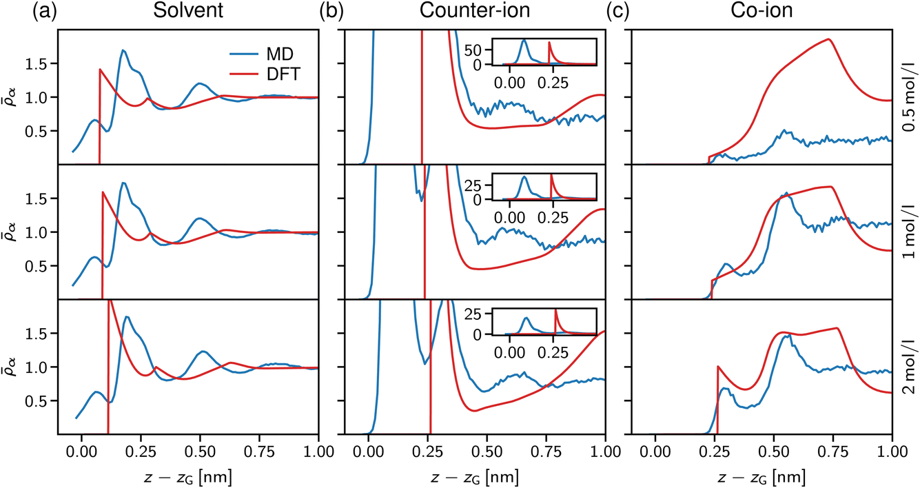 | ||
| Fig. 7 Normalised solvent and ion densities. (a) Solvent and (b, c) ion density profiles from atomistic MD simulations (blue lines) and solvent-explicit DFT calculations (orange lines). Data is shown for different salt concentrations, 0.5 mol l−1 (top), 1.0 mol l−1 (centre), and 2.0 mol l−1 (bottom), in a slit of width D = 2 nm. All data are shifted with respect to the solvent Gibbs dividing surface. | ||
In Fig. 7a, the solvent density profiles are shown for concentrations ranging from 0.5 to 2 mol l−1, revealing the well-known layering at solid substrates.77 Noteworthy, the atomistic MD data (blue lines) are hardly affected by increasing the salt concentration, with only the third layer getting more pronounced at 2 mol l−1 in line with the counter-ion layering in the bottom row of Fig. 7c. On the contrary, the simple dumbbell model employed for the DFT calculations shows increasing layering at the interface for the higher salt concentrations, but also in this case an increase of the third solvent layer density similar to the atomistic data is observed. Note that the atomistically resolved mica sheets have a rough surface according to their chemical structure, thus water can penetrate into the Gibbs surface, z − zG < 0. In contrast, the solvent dumbbells consist of hard spheres of radius 1 Å, in line with the position of the first density peak appearing in Fig. 7a. Regarding the simplicity of this model, the general trends of the solvent structure at the interface are reproduced remarkably well.
We now turn to the structural arrangement of the salt ions, shown in the middle and right columns of Fig. 7. In the atomistic simulation system, sodium counter-ions are employed, which adsorb strongly at the mica surface due to their tendency to release their hydration shell.78 However, in the DFT calculations both co- and counter-ions are treated as hard spheres with the same diameter σ± = 0.5 nm. While this leads to a remarkably good agreement for the co-ion profiles (chloride in the atomistic simulations), especially at high concentration (the bottom row in Fig. 7c), the adsorption peak of the counter-ion is not well captured in the DFT calculations. Also note that in the atomistic simulations, mica has a surface charge density that is more than three times larger than in the DFT calculations (Q = −1.8e nm−2 for mica vs. 0.5e nm−2), which explains that the area under the first counter-ion peak differs significantly between both approaches (see insets in Fig. 7b).
Our atomistic simulations indicate that the strong adsorption of sodium strongly screens the mica surface charge, reflected by nearly constant ion density profiles behind the second co-ion density peaks in Fig. 7c. As noted by Graham,79 the first strong adsorption layer of the partially hydrated sodium is not captured within the Stern layer of classical double layer theory; correspondingly, the two maxima in the counter-ion density profiles define the inner and outer Helmholtz planes,80 which are present also in the solvent-explicit DFT calculations, although differing significantly in their distance due to the different ion diameter. The co-ion profiles at high concentration (the bottom row in Fig. 7c) agree well for the first two layers and the distance between the two maxima of about 2 nm corresponds to a solvent molecular size. Thus, we conclude that electrostatic and ion-specific effects dominate the magnitude of adsorption, whereas steric effects including the solvent molecules determine the structure close to the interface at charged surfaces.
The specific effects due to adsorption can be further quantified in the context of the Gibbs surface excess, cf. eqn (10). In the presence of a charged interface, the counter-ions need to be accounted for explicitly to obtain a thermodynamic consistent interface definition. Taking the solvent as reference for the Gibbs surface allows us to define an effective slit width in a simulation box of length Lz normal to the interface, from eqn (12)
 | (12) |
Using the ion pair density ρ = ρ+ + ρ−, the salt surface excess then directly follows from eqn (10) to give eqn (13)
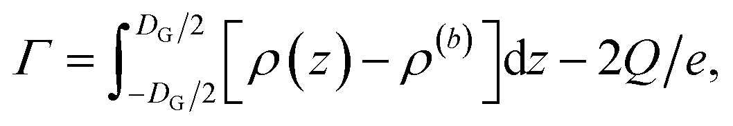 | (13) |
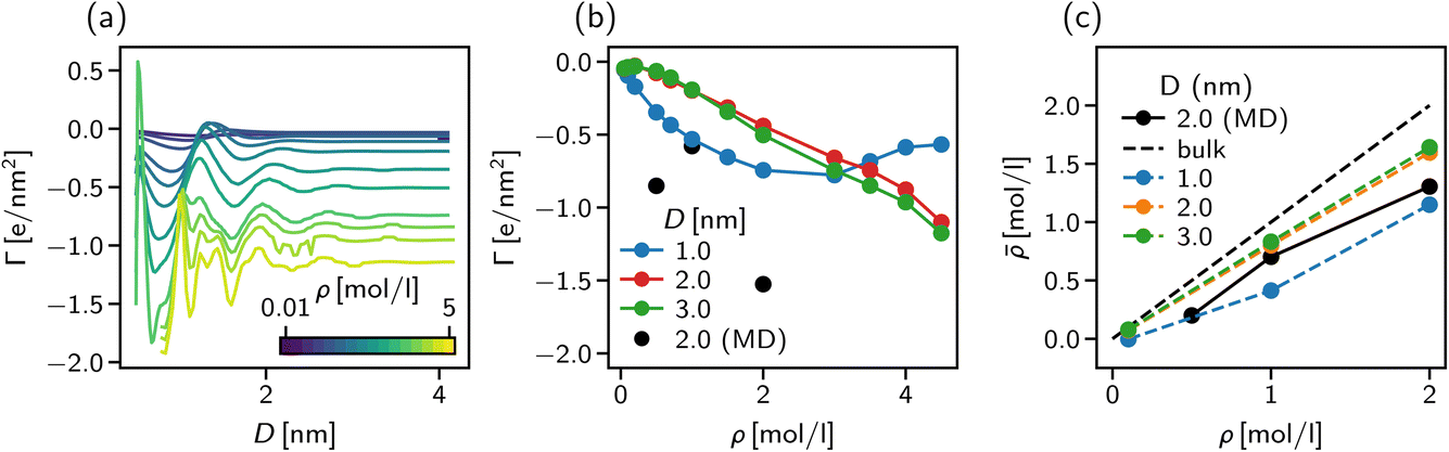 | ||
| Fig. 8 Surface excess and effective concentration in solvent-explicit simulations. (a) Surface excess of ionic species in the explicit DFT model as a function of slit width. The excess is calculated with respect to the Gibbs dividing surface of the solvent species. (b) Surface excess of ionic species in the explicit DFT model as a function of bulk concentration. The three black points represent the results of the molecular dynamics simulations. (c) Effective concentration of the ionic species inside the slit as a function of bulk concentration. | ||
The strong negative surface excess is qualitatively confirmed by our atomistic MD simulations, shown in Fig. 8b as block circles for the three concentrations considered. Whereas the DFT calculations only show a non-monotonic behaviour of Γ vs. the bulk concentration, the surface excess is expected to reveal a more complex behaviour for the atomistic system since ion-specific effects and molecular degrees of freedom are not taken into account in our DFT calculations.
The importance of addressing the solvent composition in confinement is highlighted in Fig. 8c, where we show the solvent composition in terms of the effective concentration = Nion/Ns in the pore vs. the corresponding value in bulk for different slit width D. The bisector corresponds to the trivial assumption of equal amounts of salt inside the pore as in the bulk. The fact that for increasing bulk concentration, deviates more strongly from the bisector, can be explained by the increasing surface excess as shown in Fig. 8a and b. The deviation between the trivial assumption and the actual salt ion number is up to a factor of two for D = 1 nm. Thus, to compare atomistic simulations of confined complex liquids to experimental data or theoretical models, the chemical potential of all species needs to be controlled carefully. While the approach presented here is capable of determining the right composition at high accuracy, its severe computational cost renders it unfeasible for practical application such as the study of underscreening in the pressure decay length. We found, however, that our solvent-explicit DFT calculations reproduce remarkably well the qualitative behaviour of atomistic simulations employing the extrapolation of chemical potentials for mixture compositions. Thus, we use in the next section solvent-explicit and -implicit DFT calculations to study the influence of an explicit solvent on ionic screening.
| P(D) ≈ Pb + Ae−D/ξcos(2πD/Λ + ϕ), | (14) |
The results are shown in Fig. 9. Panel (a) of this figure demonstrates that, perhaps surprisingly, the implicit and explicit solvent models lead to the same values of the decay lengths ξ. The agreement is due to the fact that, in this regime, the screening is determined by electrostatic interactions, which are the same in both models. In line with earlier work, the screening length increases and shows the scaling behaviour given by eqn (2) with exponent n = 1.5.34,40
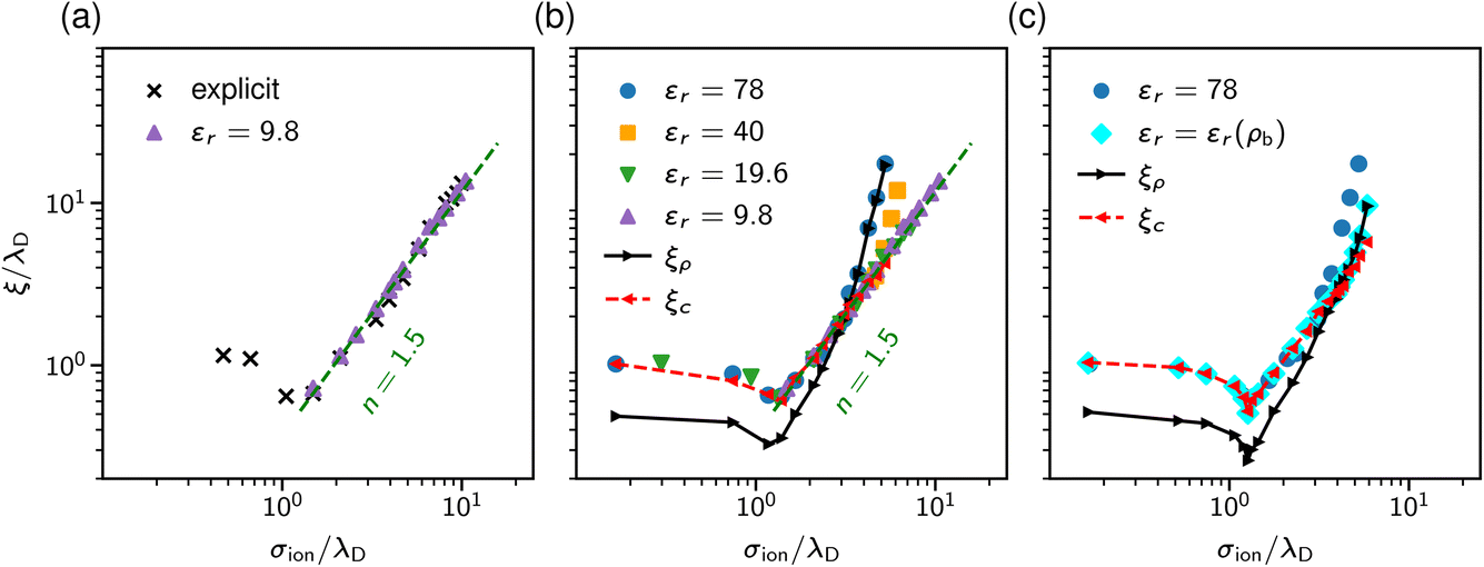 | ||
| Fig. 9 Screening lengths from DFT. Screening lengths are divided by the Debye length λD and plotted as a function of the ion diameter divided by λD. (a) Screening lengths for an explicit and implicit solvent model with the same relative dielectric permittivity εr = 9.8. (b) Screening lengths for several values of εr. The black and red symbols and lines show the decay lengths of the total and charge density profiles at a single wall for εr = 78. (c) Screening lengths for concentration-dependent and constant dielectric permittivity. The black and red symbols and lines show the decay lengths of the total and charge density profiles at a single wall in the case of the concentration dependent permittivity. | ||
Since both models lead to the same screening lengths, we consider only the implicit solvent model in the following. Fig. 9b shows the screening lengths for different values of εr. This figure demonstrates that ξ is independent of εr for intermediate concentrations, but there are systematic deviations as the concentration increases.
To understand these deviations, in addition to ξ extracted from the pressure, Fig. 9b presents the decay lengths of the number and charge density profiles, ξρ and ξc, at a single wall. At low concentrations, ξc > ξρ, hence the charge density determines the leading decay length and we found ξ ≈ ξc. As the concentration increases, there is a crossover to density-dominated screening, i.e., ξρ > ξc. In this regime, we obtained ξ ≈ ξρ. The crossover shifts toward higher concentrations as εr decreases because the decreased εr enhances the electrostatic interactions.
So far, we assumed a constant dielectric permittivity εr, while it is known that εr depends on the salt concentration ρ.83–87 To study how this dependence affects electrostatic screening, we considered two models with εr = 78 and εr(ρ) = −0.031ρ3 + 1.322ρ2 − 13.44ρ + 80.84, which describes the measured dielectric permittivity as a function of the concentration of NaCl at T = 293 K (see ref. 87). Fig. 9c shows that the concentration dependence of the relative permittivity does not affect the screening lengths at intermediate concentrations, in line with the MSA results of Rotenberg et al.40 However, the crossover to the density-dominated regime is noticeably shifted towards higher concentrations. This shift is because the presence of ions reduces εr, thus enhancing the electrostatic interactions, which extends the region of the electrostatics-dominated screening.
4 Conclusions
Screening in ionic fluids is essential for many fundamental processes and industrial applications. Nevertheless, our understanding of screening in concentrated electrolytes and ILs remains incomplete. Recent SFB experiments have challenged our knowledge of screening in dense ionic systems by reporting screening lengths about one order of magnitude larger than expected. This effect was ascribed to the bulk properties of ionic systems and termed underscreening, or recently even anomalous underscreening, to pinpoint that the system is underscreened compared to what is expected based on classical theories or the Debye ionic cloud model, respectively. We have reviewed the experimental, theoretical and simulation work attempting to resolve this apparent under-screening paradox. This overview indicates that there is no solid evidence from theory and simulations to support the (anomalous) underscreening as a bulk property of concentrated ionic systems.New theoretical and simulation work motivated by underscreening experiments brought new insight and new questions into our understanding of ionic screening. Experiments on underscreening suggested a cubic scaling of the screening lengths with the Debye length (eqn (2) with n = 3). With a few exceptions,27,41,42 which still need careful examination, such cubic scaling has yet to be found in theory or simulations in the experimentally relevant parameter space. Instead, a selection of other scaling exponents have been reported, viz., n = 1 (ref. 40, 41 and 58), n = 2 (ref. 35, 41 and 58), n ≈ 1.3 (ref. 57), n = 1.5 (ref. 34, 40 and 41 and this work), and n = 5 (ref. 41), depending on the model and method used. Future work will show whether there is universal scaling at all, and what its physical significance is.
While reviewing the previous results on ionic screening, we noted the scarcity of studies on how solvent, ion–surface interactions and confinements influence ionic screening. We have attempted to fill this gap. We used molecular dynamics simulations at controlled chemical potential of all components and classical density functional theory to investigate how the solvent dielectric properties affect the decay length of the force exerted on the confining walls. Comparison between atomistic MD and solvent-explicit DFT simulations revealed that the solvent and ion structure differs from the behaviour in bulk – as expected – only close to the surface. Furthermore, it is – at least on a qualitative level – dominated by steric, excluded volume effects and not by ion- or surface- specific interactions, thus rendering the coarse-grained DFT calculations a viable approach to study underscreening since the usual way to control chemical composition on an atomistic resolution is computationally too demanding, and therefore infeasible. Using DFT, we found that, somewhat surprisingly, in the electrostatics-dominated regime, the screening length is virtually independent of (i) whether the solvent is modelled implicitly or is spatially resolved, (ii) whether dielectric permittivity εr depends on the ion concentration or not, and (iii) on the value of εr. However, our calculations revealed that a crossover to the hard-core dominated regime, which occurs at higher concentrations, depends sensitively on the details of the solvent (Fig. 9).
We hope this overview and our new results on the solvent effects will motivate further experimental, theoretical, and simulation work on screening in concentrated ionic systems.
Data availability
The data supporting the findings of this research, including the input scripts for the atomistic simulatios, the scripts to produce the figures presented in the paper, and the custom software used in the research, are available at https://doi.org/10.18419/darus-3551.Conflicts of interest
There are no conflicts to declare.Acknowledgements
A. S., C. H. and H. J. were funded by the Deutsche Forschungsgemeinschaft (DFG, German Research Foundation) under Germany's Excellence Strategy – EXC 2075 – 390740016 and SFB 1333/2 – 358283783. S. K. acknowledges the financial support by NCN Grants 2020/39/I/ST3/02199 and 2021/40/Q/ST4/00160.References
- J. L. Seifter and H.-Y. Chang, Physiology, 2017, 32, 367–379 CrossRef CAS PubMed.
- C. M. Armstrong, Proc. Natl. Acad. Sci. U. S. A., 2003, 100, 6257–6262 CrossRef CAS PubMed.
- S. Kondrat, U. Krauss and E. von Lieres, Curr. Res. Chem. Biol., 2022, 2, 100031 CrossRef CAS.
- S. Kondrat and E. von Lieres, in Multienzymatic Assemblies: Methods and Protocols, ed. H. Stamatis, Springer US, New York, NY, 2022, pp. 27–50 Search PubMed.
- B. Drukarch, H. A. Holland, M. Velichkov, J. J. G. Geurts, P. Voorn, G. Glas and H. W. de Regt, Prog. Neurobiol., 2018, 169, 172–185 CrossRef PubMed.
- M. Peyrard, J. Biol. Phys., 2020, 46, 327–341 CrossRef PubMed.
- M. W. Berchtold, H. Brinkmeier and M. Müntener, Physiol. Rev., 2000, 80, 1215–1265 CrossRef CAS PubMed.
- I. Y. Kuo and B. E. Ehrlich, Cold Spring Harbor Perspect. Biol., 2015, 7, a006023 CrossRef PubMed.
- J. A. Rall, Am. J. Physiol.: Adv. Physiol. Educ., 2022, 46, 481–490 Search PubMed.
- A. J. Greer, J. Jacquemin and C. Hardacre, Molecules, 2020, 25, 5207 CrossRef CAS PubMed.
- G. Kaur, H. Kumar and M. Singla, J. Mol. Liq., 2022, 351, 118556 CrossRef CAS.
- M. Watanabe, M. L. Thomas, S. Zhang, K. Ueno, T. Yasuda and K. Dokko, Chem. Rev., 2017, 117, 7190–7239 CrossRef CAS PubMed.
- G. Jeanmairet, B. Rotenberg and M. Salanne, Chem. Rev., 2022, 122, 10860–10898 CrossRef CAS PubMed.
- J. Wu, Chem. Rev., 2022, 122, 10821–10859 CrossRef CAS PubMed.
- M. Janssen, T. Verkholyak, A. Kuzmak and S. Kondrat, J. Mol. Liq., 2023, 371, 121093 CrossRef CAS.
- A. Paul, S. Muthukumar and S. Prasad, J. Electrochem. Soc., 2020, 167, 037511 CrossRef CAS.
- T. Welton, Coord. Chem. Rev., 2004, 248, 2459–2477 CrossRef CAS.
- H. Olivier-Bourbigou, L. Magna and D. Morvan, Appl. Catal., A, 2010, 373, 1–56 CrossRef CAS.
- P. Attard, Phys. Rev. E: Stat. Phys., Plasmas, Fluids, Relat. Interdiscip. Top., 1993, 48, 3604–3621 CrossRef CAS PubMed.
- R. L. de Carvalho and R. Evans, Mol. Phys., 1994, 83, 619–654 CrossRef.
- J. G. Kirkwood, Chem. Rev., 1936, 19, 275–307 CrossRef CAS.
- M. A. Gebbie, M. Valtiner, X. Banquy, E. T. Fox, W. A. Henderson and J. N. Israelachvili, Proc. Natl. Acad. Sci. U. S. A., 2013, 110, 9674–9679 CrossRef CAS PubMed.
- M. A. Gebbie, H. A. Dobbs, M. Valtiner and J. N. Israelachvili, Proc. Natl. Acad. Sci. U. S. A., 2015, 112, 7432–7437 CrossRef CAS PubMed.
- A. M. Smith, A. A. Lee and S. Perkin, J. Phys. Chem. Lett., 2016, 7, 2157–2163 CrossRef CAS PubMed.
- A. A. Lee, C. S. Perez-Martinez, A. M. Smith and S. Perkin, Faraday Discuss., 2017, 199, 239–259 RSC.
- A. A. Lee, C. S. Perez-Martinez, A. M. Smith and S. Perkin, Phys. Rev. Lett., 2017, 119, 026002 CrossRef PubMed.
- A. Härtel, M. Bültmann and F. Coupette, Phys. Rev. Lett., 2023, 130, 108202 CrossRef PubMed.
- S. Kumar, P. Cats, M. B. Alotaibi, S. C. Ayirala, A. A. Yousef, R. van Roij, I. Siretanu and F. Mugele, J. Colloid Interface Sci., 2022, 622, 819–827 CrossRef CAS PubMed.
- R. Evans, R. J. F. L. de Carvalho, J. R. Henderson and D. C. Hoyle, J. Chem. Phys., 1994, 100, 591–603 CrossRef CAS.
- S. Perkin, M. Salanne, P. Madden and R. Lynden-Bell, Proc. Natl. Acad. Sci. U. S. A., 2013, 110, E4121 CrossRef CAS PubMed.
- A. A. Lee, D. Vella, S. Perkin and A. Goriely, J. Phys. Chem. Lett., 2015, 6, 159–163 CrossRef CAS PubMed.
- C. Holm and S. Kondrat, Journal Club for Condensed Matter Physics, 2022 DOI:10.36471/JCCM_November_2022_02.
- J. Zeman, S. Kondrat and C. Holm, J. Chem. Phys., 2021, 155, 204501 CrossRef CAS PubMed.
- P. Cats, R. Evans, A. Härtel and R. van Roij, J. Chem. Phys., 2021, 154, 124504 CrossRef CAS PubMed.
- R. M. Adar, S. A. Safran, H. Diamant and D. Andelman, Phys. Rev. E, 2019, 100, 042615 CrossRef CAS PubMed.
- M. Han and R. M. Espinosa-Marzal, J. Phys. Chem. C, 2018, 122, 21344–21355 CrossRef CAS.
- P. Gaddam and W. Ducker, Langmuir, 2019, 35, 5719–5727 CrossRef CAS PubMed.
- H. Yuan, W. Deng, X. Zhu, G. Liu and V. S. J. Craig, Langmuir, 2022, 38, 6164–6173 CrossRef CAS PubMed.
- T. Baimpos, B. R. Shrestha, S. Raman and M. Valtiner, Langmuir, 2014, 30, 4322–4332 CrossRef CAS PubMed.
- B. Rotenberg, O. Bernard and J.-P. Hansen, J. Phys.: Condens. Matter, 2018, 30, 054005 CrossRef PubMed.
- A. Ciach and O. Patsahan, J. Mol. Liq., 2023, 377, 121453 CrossRef CAS.
- A. Ciach and O. Patsahan, J. Phys.: Condens. Matter, 2021, 33, 37LT01 CrossRef CAS PubMed.
- O. Patsahan and A. Ciach, ACS Omega, 2022, 7, 6655–6664 CrossRef CAS PubMed.
- N. G. van Kampen, Phys. Rev., 1964, 135, A362–A369 CrossRef.
- C. Ebner, W. F. Saam and D. Stroud, Phys. Rev. A: At., Mol., Opt. Phys., 1976, 14, 2264–2273 CrossRef.
- R. Evans, Adv. Phys., 1979, 28, 143–200 CrossRef CAS.
- Y. Rosenfeld, Phys. Rev. Lett., 1989, 63, 980–983 CrossRef CAS PubMed.
- R. Roth, R. Evans, A. Lang and G. Kahl, J. Phys.: Condens. Matter, 2002, 14, 12063–12078 CrossRef CAS.
- H. Hansen-Goos and R. Roth, J. Phys.: Condens. Matter, 2006, 18, 8413–8425 CrossRef CAS PubMed.
- R. Roth, J. Phys.: Condens. Matter, 2010, 22, 063102 CrossRef PubMed.
- S. A. Brazovskii, Phase Transition of an Isotropic System to a Nonuniform State, 30 Years of the Landau Institute – Selected Papers, World Scientific, Singapore, 1996, vol. 11, pp. 109–113 Search PubMed.
- S. A. Brazovskii, J. Exp. Theor. Phys., 1975, 41, 85 Search PubMed.
- R. Kjellander, Soft Matter, 2019, 15, 5866–5895 CAS.
- R. Kjellander, J. Chem. Phys., 2018, 148, 193701 CrossRef PubMed.
- R. Kjellander and D. J. Mitchell, Chem. Phys. Lett., 1992, 200, 76–82 CrossRef CAS.
- R. Kjellander and D. J. Mitchell, J. Chem. Phys., 1994, 101, 603–626 CrossRef CAS.
- S. W. Coles, C. Park, R. Nikam, M. Kanduč, J. Dzubiella and B. Rotenberg, J. Phys. Chem. B, 2020, 124, 1778 CAS.
- J. Zeman, S. Kondrat and C. Holm, Chem. Commun., 2020, 56, 15635–15638 RSC.
- F. Coupette, A. A. Lee and A. Härtel, Phys. Rev. Lett., 2018, 121, 075501 CrossRef CAS PubMed.
- P. A. Bonnaud, B. Coasne and R. J.-M. Pellenq, J. Chem. Phys., 2012, 137, 064706 CrossRef PubMed.
- R. W. Zwanzig, J. Chem. Phys., 1954, 22, 1420–1426 CrossRef CAS.
- A. Schlaich, A. P. dos Santos and R. R. Netz, Langmuir, 2019, 35, 551–560 CrossRef CAS PubMed.
- A. Schlaich, B. Kowalik, M. Kanduč, E. Schneck and R. R. Netz, in Computational Trends in Solvation and Transport in Liquids, ed. G. Sutmann, J. Grotendorst, G. Gompper and D. Marx, Forschungszentrum Jülich GmbH, Jülich, 2015, vol. 28 of IAS Series, pp. 155–185 Search PubMed.
- E. Schneck, F. Sedlmeier and R. R. Netz, Proc. Natl. Acad. Sci. U. S. A., 2012, 109, 14405–14409 CrossRef CAS PubMed.
- M. Kanduč, A. Schlaich, A. H. de Vries, J. Jouhet, E. Maréchal, B. Demé, R. R. Netz and E. Schneck, Nat. Commun., 2017, 8, 14899 CrossRef PubMed.
- H. Heinz, H. Koerner, K. L. Anderson, R. A. Vaia and B. L. Farmer, Chem. Mater., 2005, 17, 5658–5669 CrossRef CAS.
- R. Fuentes-Azcatl and J. Alejandre, J. Phys. Chem. B, 2014, 118, 1263–1272 CrossRef CAS PubMed.
- P. Loche, P. Steinbrunner, S. Friedowitz, R. R. Netz and D. J. Bonthuis, J. Phys. Chem. B, 2021, 125, 8581–8587 CrossRef CAS PubMed.
- D. Henderson, D.-e. Jiang, Z. Jin and J. Wu, J. Phys. Chem. B, 2012, 116, 11356–11361 CrossRef CAS PubMed.
- C. E. Woodward, J. Chem. Phys., 1991, 94, 3183–3191 CrossRef CAS.
- Y.-X. Yu and J. Wu, J. Chem. Phys., 2002, 117, 10156–10164 CrossRef CAS.
- J. Wu, T. Jiang, D.-e. Jiang, Z. Jin and D. Henderson, Soft Matter, 2011, 7, 11222–11231 RSC.
- Y.-X. Yu and J. Wu, J. Chem. Phys., 2002, 116, 7094–7103 CrossRef CAS.
- Y.-X. Yu and J. Wu, J. Chem. Phys., 2002, 117, 2368–2376 CrossRef CAS.
- J. Mairhofer and J. Gross, Fluid Phase Equilib., 2017, 444, 1–12 CrossRef CAS.
- D. K. Chattoraj and K. S. Birdi, Adsorption and the Gibbs Surface Excess, Plenum Press, New York, 1984 Search PubMed.
- J. N. Israelachvili and R. M. Pashley, Nature, 1983, 306, 249–250 CrossRef CAS.
- H. Sakuma, T. Kondo, H. Nakao, K. Shiraki and K. Kawamura, J. Phys. Chem. C, 2011, 115, 15959–15964 CrossRef CAS.
- D. C. Grahame, Chem. Rev., 1947, 41, 441–501 CrossRef CAS PubMed.
- G. Gonella, E. H. G. Backus, Y. Nagata, D. J. Bonthuis, P. Loche, A. Schlaich, R. R. Netz, A. Kühnle, I. T. McCrum, M. T. M. Koper, M. Wolf, B. Winter, G. Meijer, R. K. Campen and M. Bonn, Nat. Rev. Chem., 2021, 1–20 Search PubMed.
- A. M. Smith, K. R. J. Lovelock, N. N. Gosvami, T. Welton and S. Perkin, Phys. Chem. Chem. Phys., 2013, 15, 15317 RSC.
- F. G. Donnan, Chem. Rev., 1924, 1, 73–90 CrossRef CAS.
- R. Buchner, G. T. Hefter and P. M. May, J. Phys. Chem. A, 1999, 103, 1–9 CrossRef CAS.
- B. Hess, C. Holm and N. van der Vegt, Phys. Rev. Lett., 2006, 96, 147801 CrossRef PubMed.
- M. Sega, S. S. Kantorovich, C. Holm and A. Arnold, J. Chem. Phys., 2014, 140, 211101 CrossRef CAS PubMed.
- M. Valiskó and D. Boda, J. Chem. Phys., 2014, 140, 234508 CrossRef PubMed.
- N. Gavish and K. Promislow, Phys. Rev. E, 2016, 94, 012611 CrossRef PubMed.
Footnotes |
| † Electronic supplementary information (ESI) available: Further details on the simulation methods, atomistic simulations, chemical potential measurement and determination of the dielectric constant in the solvent-explicit DFT calculations. See DOI: https://doi.org/10.1039/d3fd00043e |
| ‡ These authors contributed equally to this work. |
| This journal is © The Royal Society of Chemistry 2023 |