
 Open Access Article
 This Open Access Article is licensed under a
 Creative Commons Attribution 3.0 Unported Licence
From Goldilocks to twin peaks: multiple optimal regimes for quantum transport in disordered networks
Alexandre R.
Coates
 a,
Brendon W.
Lovett
b and
Erik M.
Gauger
*a
a,
Brendon W.
Lovett
b and
Erik M.
Gauger
*a
aSUPA, Institute of Photonics and Quantum Sciences, Heriot-Watt University, Edinburgh EH14 4AS, UK. E-mail: e.gauger@hw.ac.uk
bSUPA, School of Physics and Astronomy, University of St Andrews, St Andrews KY16 9SS, UK
First published on 22nd March 2023
Abstract
Understanding energy transport in quantum systems is crucial for an understanding of light-harvesting in nature, and for the creation of new quantum technologies. Open quantum systems theory has been successfully applied to predict the existence of environmental noise-assisted quantum transport (ENAQT) as a widespread phenomenon occurring in biological and artificial systems. That work has been primarily focused on several ‘canonical’ structures, from simple chains, rings and crystals of varying dimensions, to well-studied light-harvesting complexes. Studying those particular systems has produced specific assumptions about ENAQT, including the notion of a single, ideal, range of environmental coupling rates that improve energy transport. In this paper we show that a consistent subset of physically modelled transport networks can have at least two ENAQT peaks in their steady state transport efficiency.
1 Introduction
Energy transport occurs in many contexts: from circuits and molecular junctions to processes like photosynthesis and the electron transport chain in biology.1–8 In 2008 the specifics of Environmental Noise-Assisted Quantum Transport (ENAQT) were first laid out in both artificial and natural schema.9–12 Since then there has been a proliferation of research into the interplay of coherent quantum transport and noise in many systems,13–15 such as the role environmental phonon coupling can have in overcoming the effects of coherent localisation.16–19 From these studies and others, an intuition has been established that ENAQT produces a single ‘Goldilocks zone’20–22 where dephasing overcomes limits inherent to fully coherent dynamics, but is not sufficiently aggressive to spoil its favourable transport characteristics, such as those brought about by constructive interference.The study of quantum transport in these various open systems has been typically carried out on only a few model systems, and some common network structures; notable exceptions also considering randomly generated networks include ref. 15 and 23–25. In the context of biological photosynthetic exciton energy transport this is often the Fenna–Matthew–Olson complex (FMO),22,26–29 and in quantum technologies we see (disordered) chains and lattices used to simulate many transport scenarios.14–18,30–35 We see across these contexts that energetic disorder is common in many systems, with the specifics of these energy landscapes having a strong effect on quantum transport.16,23,25,36
Recent work introducing the concept of ‘population uniformisation’ has made the varying transport behaviour between fully coherent and fully classical limits explicit.37 Population uniformisation states that the variance in on-site populations has a similar qualitative character to the transport efficiency of open quantum systems, and is minimised when transport efficiency is maximised, even in the presence of disorder or repulsive interactions.18,37 While this framework explicitly frames things in terms of moving from coherent wavefunctions to classical diffusion and Fick's Law, we yet again see the same, singly peaked ENAQT transport efficiency on the standard systems, including the FMO complex.38
In this paper we systematically investigate optimal noise rates across randomly generated transport networks, and show that many have at least two ENAQT peaks or ‘Goldilocks Zones’ where their transport efficiency is maximised. Our networks are made of two-level systems, which we model as point dipoles. We arrange these sites with realistic spacing and effective dipole moments to ensure the relevance of our results, and consider both uniform and normally distributed energy landscapes.
2 Transport model
2.1 Network setup
We set up each system as follows: first we define a sphere with a fixed radius of 10 nm, and place two sites at opposite ends of the sphere to act as injection and extraction sites. We then fill the volume with six additional sites with random positions and dipole orientations to produce a disordered but fully connected network, a similar setup and approach has been utilised in prior works.23,30,39Fig. 1 shows a typical dipole network generated in this way. | ||
| Fig. 1 Illustration of a typical dipole system: a fixed volume with injection and extraction sites in at the poles, and randomly oriented and positioned sites within the volume. The system is then coupled to phonon environments with varying strengths (Γ), and the transport efficiency (η) measured. On the right we show transport efficiency curves from a selection of randomly generated networks modelled with phenomenological pure dephasing that exhibit multiple maxima in their transport efficiency. | ||
Every site is modelled with an identical dipole moment, we use the effective dipole moments from the bacteriochlorophylls in the FMO complex  .27,40–42
With the structure established we can consider the dipole–dipole interactions,
 | (1) |
To generate the dipole on-site energies we use an average on-site energy ![[small epsilon, Greek, macron]](https://www.rsc.org/images/entities/i_char_e0c6.gif) = 1.5498 eV (12
= 1.5498 eV (12![[thin space (1/6-em)]](https://www.rsc.org/images/entities/char_2009.gif) 500 cm−1), and will later also sample them from a normal distribution with a standard deviation of 1%, so σ = 0.0155 eV, very similar to the energies and disorder found in the FMO complex.40 The default values we use are summarised in Table 1.
500 cm−1), and will later also sample them from a normal distribution with a standard deviation of 1%, so σ = 0.0155 eV, very similar to the energies and disorder found in the FMO complex.40 The default values we use are summarised in Table 1.
| Radius (nm) | N | r min (nm) | |d| (e nm) |
(eV) |
σ (eV) |
|---|---|---|---|---|---|
| 10 | 8 | 1 | 0.11403 | 1.5498 | 0.0155 |
With the on-site energies and dipole–dipole interactions defined we can construct the Hamiltonian. We assume there is only a single excitation in the system at any time and construct the following excitonic Hamiltonian
 | (2) |
2.2 Dynamics
To look at the effect of the environment and finite temperatures on transport properties, we use the full non-secular Bloch–Redfield master equation47,48 | (3) |
 into the Hamiltonian eigenbasis and Smn(ω) defines the noise-power spectrum associated with the system–environment interaction.30,47,48 The noise-power spectrum function is
 | (4) |
 defines Bose–Einstein statistics at a given phonon inverse temperature β, Θ(ω) is the Heaviside function, allowing phonon-assisted transitions from higher to lower eigenenergies (ω > 0), and
  is the phonon spectral density.48 In this work we use the Drude–Lorentz spectral density, which has previously been used to model excitonic transfer in light harvesting complexes,49,50
 | (5) |
Finally, we have  which is the dissipator superoperator
 | (6) |
To model extraction and injection, a shelf state is appended to the system. The extraction operator Aext projects population from the extraction site to the shelf state, Aext = σshelf+σext−, and then that population is re-injected from the shelf state back onto the injection site with the injection operator Ainj = σinj+σshelf−. Injection and extraction are matched, γext,inj = 0.1 eV, changing this value generally changes quantitative values but not the qualitative behaviour.37
To complement the Redfield calculations, we also carry out phenomenological pure dephasing calculations with the Lindblad master equation47,51,52
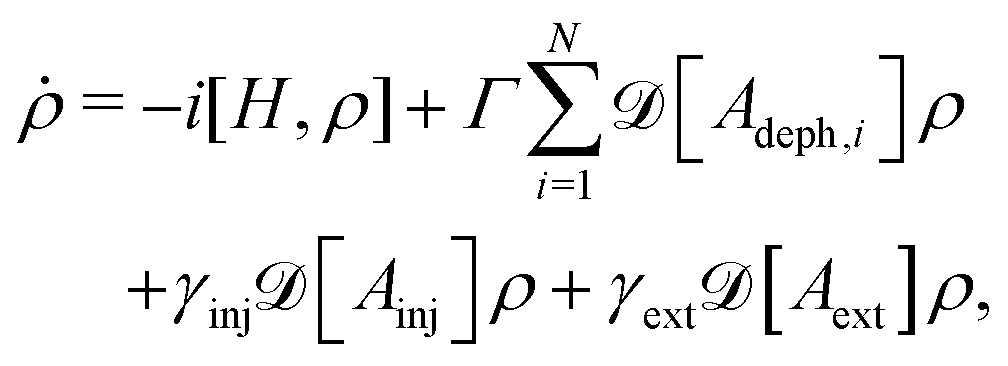 | (7) |
 .48 All other symbols have the same meaning as in eqn (3). This approach is equivalent to the nonsecular Bloch–Redfield master equation for an infinite temperature and a flat spectral density.25
We focus here on the steady state ρss which is found by calculating the null vector of the system evolution Liouvillian. Our figure of merit then is the excited steady state population on the extraction site
| η = 〈extraction|ρss|extraction〉. | (8) |
This is motivated by the strong correspondence found in prior work between dynamical and steady state transport properties,18,53 as well as further studies suggesting that the steady state is more natural for photosynthetic systems.2,54,55 The steady state approach also allows us to avoid any confusion that could arise from the influence of transient effects when comparing different networks.
For each network considered in this paper, we were interested in how this transport efficiency η changes with Γ, the noise rate from coupling to the environment. To do this we considered a large range of noise rates  and for each value recorded η as well as the full steady state population. This range of Γ was chosen as it was broad enough to capture the values where η has maxima for our networks, and additionally show the transport efficiency decreasing outside these peaks as shown in Fig. 1.
These results were then filtered to ensure validity, all data presented here has passed checks on the unity of the steady state trace, non-negativity of on-site populations and steady state eigenvalues (see Appendix K). From that point we could perform simple peak-finding calculations for each network and spectral density to directly identify in which cases there was more than one optimal noise rate or peak in the transport efficiency curves, and how often this occurred.
3 Results
3.1 Environmental effects
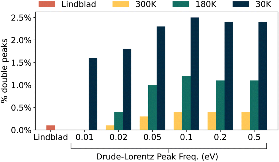
We generated several ensembles of 1000 dipole networks, each comprising two fixed and six randomly located sites. For our Redfield calculations the key spectral density parameters are the temperature, and the peak frequency of the Drude–Lorentz spectral density (τ−1). Lindbladian pure dephasing acts as our infinite temperature limit, being equally present at all frequencies.We start by considering an ensemble of networks with identical splitting between the two levels on each site, and see how many networks have multiple maxima in their transport efficiency. This approach lets us compare our results to prior works that have made the same assumption of uniform on-site energies when modelling disordered molecular networks and other complexes with dipole interactions.24,39,56
Fig. 2 shows a surprising result, contrary to prior wisdom we consistently find about 6% of networks have multiple peaks in their transport efficiency, regardless of the spectral density or temperature. This illustrates that these fully connected networks can have multiple maxima in their transport efficiency, but neglects the importance of on-site energies in transport.25 We consider the effects of varied on-site energies in Fig. 3, where the energies are normally distributed as described in Table 1.
 | ||
| Fig. 2 Percentage of dipole networks showing double-ENAQT behaviour in networks with uniform on-site energies. We see only a slight sensitivity to the peak frequency in this case, and a slight increase in the behaviour at low temperatures. This is likely because the eigenenergy splittings are quite small when the on-site energies are identical, and as such the transport behaviour depends on the near zero behaviour of the Drude–Lorentz spectral density, which is a relatively stable region. | ||
 | ||
| Fig. 3 Percentage of networks with normally distributed energies showing double-peaked ENAQT behaviour. The lower the temperature and the higher the environment peak frequency, the more often we observe this phenomenon. There is a much larger sensitivity to the spectral density than in the energetically uniform case. | ||
Fig. 2 and 3 show our main results from this paper. We see that in every situation we simulate, a sizeable subset of our networks have two peaks in the their transport efficiency. The Drude–Lorentz peak frequency has a slight effect on how often we observe this behaviour, but there is a more pronounced sensitivity to temperature. The lower the temperature, the more often we see this behaviour. By extension, this is seen least often – but still clearly represented – in the Lindblad pure dephasing limit. We show what proportion of these results occur within measured FMO reorganisation energies in Appendix G.
We note that this double peaked phenomenon generally occurs more frequently in the energetically uniform ensemble. We attribute this to energetic disorder producing greater localisation. Meaning that not only are the energetic differences between eigenstates larger, but also those eigenstates are more tightly confined to specific sites. This greater spatial confinement means there are fewer pathways from injection site to extraction site. The greater energetic differences also raise the chance of some eigenstates being so far detuned that they are effectively inaccessible given the finite range of noise rates Γ we consider.
3.2 Structural effects
As shown on the right of Fig. 1, different networks have transport efficiency curves that take a variety of forms. The relative prominence and position of each transport efficiency peak varies. In some cases peaks are very well separated with a pronounced dip between them. In other cases the two are barely distinguishable, almost smearing into each other. This suggests a strong structural dependence between the form of the curves and the Hamiltonians of their respective networks.We closely inspected networks such as the one in Fig. 4, which produce double peaks across a wide range of temperatures and Drude–Lorentz peak frequencies, to identify what key features might be correlated with having multiple peaks in the transport efficiency of a system. See Appendix F for the physical properties of the network.
 | ||
| Fig. 4 A system where we see double-peaked ENAQT for all forms of spectral density we consider. (a) Shows the dipole positions and orientations for this network, with the z-axis pointing upwards, and then out of the page (tilted by π/2) in the top and bottom plot, respectively. (b) Shows the transport efficiency in all our cases and (c) shows the network Hamiltonian eigenstates, with eigenenergies on the y-axis and site indices on the x-axis (0 and 1 are the injection and extraction sites, respectively). The size of the diamonds indicate the support of the eigenstate on that site. | ||
We did not find any strong geometric dependence across networks with multiple maxima in their transport efficiency, but we identified consistent features in the system eigenstates. Specifically, these systems often have one or more large gaps in their eigenenergy distributions, as shown in Fig. 4(c).
3.3 Discussion
An intuitive and tempting interpretation of the multiple optimal transport regimes would be that two broad sets of energy scales are important: the width of each band of eigenenergies, and the separation between bands. The intuition from this being that there is an initial path with an ideal environmental coupling for ENAQT. However, as phonon couplings become larger, eigenstates that were previously far–detuned become more accessible. If the new path is more efficient for exciton transport, then a new peak in the transport efficiency can be observed. Both the energetically uniform and non-uniform ensembles consistently have these gaps in their spectra, induced by the dipole–dipole interactions between sites, and if present, differences in on-site energies.Testing this hypothesis in Appendix A we do indeed find a positive correlation with the relative standard deviation of eigenenergy splittings. However the change in the fraction of multiply peaked networks remains modest, suggesting there are other factors at play. In the following we briefly summarise how doubly peaked behaviour correlates with some other aspects.
In Appendix B we tested the energetic separation hypothesis in another way, generating a new independent ensemble of 1000 networks where three of the dipoles have a fixed offset added to their on-site energies. This approach encourages more gaps to form in the eigenspectra and we see a modest increase in the frequency of double peaks.
We also have considered the relative energies of the injection and extraction sites in these systems. In Appendix C we show that double peaks occur more frequently when injecting at lower energies than the extraction site, suggesting it may occur more often in less efficient networks (in the sense of requiring ‘uphill’ energy transport), albeit by no means limited to those. In Appendix H we directly compare the maximum transport efficiency of single-peaked and double-peaked networks, and show that double-peaked networks have a larger spread in their transport efficiencies, but can be just as efficient as the single-peaked networks. Appendix I is then concerned with how relevant each peak is in double-peaked systems. We find that that both peaks typically have a similar prominence, though the peak at higher system-environment couplings tends to be more efficient.
Another consideration is the number of potential paths in a system from the injection site to the extraction site. We generated an ensemble of networks made of paired, disordered, nearest-neighbour chains that only connected at shared injection and extraction sites, giving only two paths across the system. In Appendix D we show that while this strongly reduces how often a network has multiple transport efficiency maxima, we do still observe it against all spectral densities. We further show in Appendix E that double peaks can be observed against Ohmic and superohmic spectral densities as well. To consider the effect of system density, in Appendix J we reduce the minimum separation between sites and the total system volume to better match the chromophoric density seen in light-harvesting complexes. Again we find a similar subset of networks with multiple optimal noise rates, though one that less favours multiple ENAQT peaks at low temperatures.
Overall, our analysis suggests there are a multitude of factors at play which can positively correlate with an increased occurrence of doubly peaked networks. The analysis in this paper has been focused on networks with double peaks as that is what we observe for these systems. We believe that more than two ENAQT peaks are possible, and that networks with more sites and potential paths from source to sink may present such behaviour. Given the large amount of parameters involved in these systems we have presented many conditions that allow for these multiple peaks to occur in a range of system geometries, but do not find any condition that strongly correlates with the multiple ENAQT peaks being present.
4 Conclusion
In this paper, we have shown that transport networks with realistic and microscopically resolved vibrational interactions frequently feature more than one optimal regime for transport efficiency. This runs counter to expectations of there being a single ‘Goldilocks zone’ in any and all cases. We observe that these multiple optimal transport regimes can occur for energetically ordered or energetically disordered networks, and occur more often in networks with less evenly spaced eigenvalues.Conflicts of interest
There are no conflicts to declare.Appendices
A Role of eigenenergy spacing disorder
Here we present statistical analysis of the role of disorder in the spacing of eigenenergies, specifically we consider the relative standard deviation where σ is the standard deviation of the eigenenergy differences, and μ is the average eigenenergy difference. We find in both our energetically uniform and energetically disordered ensembles that more disorder in eigenenergy spacings is positively correlated with an increased fraction of networks displaying two optimal transport regimes. The probability density histograms against the relative standard deviation are shown for the energetically disordered and energetically uniform ensembles in Fig. 5 and 6 respectively.
 | ||
| Fig. 5 Histogram of probability density against the relative standard deviation of network eigenenergy differences for energetically disordered networks. We see the networks with double peaks occur more often for higher amounts of disorder. We test this directly in Appendix B. | ||
 | ||
| Fig. 6 Histogram of probability density against the relative standard deviation of network eigenenergy differences for 1000 energetically uniform networks, previously described in Fig. 2. Without an energy landscape, we see a wide spread of relative standard deviations defined by the geometric properties of the networks. We see a relatively sharp maximum relative standard deviation here due to the exclusion volume or minimum distance we enforce between dipoles when generating our systems. | ||
B Networks with offset energies
Based on our intuition of double peaks being related to two effective pathways with different optimal conditions for ENAQT, we generate a new, independent ensemble of networks with two different on-site energy scales. We generate the dipole networks exactly as before, including their random on-site energies. Then for each network we randomly pick three of the bulk dipoles and shift their energy upwards by the standard deviation of our on-site energies (+15.5 meV).This adjustment to the networks increases the probability of there being a larger gap in the system eigenenergies, but leaves the geometric properties of these networks unaffected. As shown in Fig. 7, we do see some increase in double-peaked transport efficiency in most cases. Though as expected when comparing two independent datasets there are fluctuations in the trends.
 | ||
| Fig. 7 The hatched bars show percentage of dipole networks with double-ENAQT behaviour in our artificially offset networks. The coloured bars show the prior results from Fig. 3 for the normally distributed on-site energies. We see a general increase in double peaked behaviour thanks to this energy offset. | ||
C Injection and extraction energies
We also consider the importance of where the injection and extraction sites sit in the eigenenergy landscape. We index the eigenstates from lowest to highest energy (λ1→N), and record which eigenstate is most present on the injection site (λinj) and the extraction site (λext), respectively.For our networks with no double peaks, there is general symmetry. For the networks with multiple transport efficiency maxima, we see a preference for injecting at lower eigenenergies than they extract at (λinj − λext < 0). This suggests the effect will be more prominent in less efficient systems. Though we note that the effect is present broadly, also clearly occurring in networks where energy transport should be efficient along a downhill gradient. Fig. 8 shows these results for energetically disordered networks, and Fig. 9 shows the same for energetically uniform networks. We see the same trend in both results, however for the energetically uniform case the eigenstates are more delocalised, often being spread over two or more sites. As a result there are multiple cases where λinj − λext = 0 due to the sites sharing a pair of eigenstates which are equally present on the injection and extraction sites. This does not occur in the energetically disordered ensemble because of the additional localisation.
 | ||
| Fig. 8 Histogram of probability density against the difference in eigenenergy index of the injection and extraction sites for energetically disordered systems. Negative values mean the injection is below the extraction. | ||
 | ||
| Fig. 9 Histogram of probability density against the difference in eigenenergy index of the injection and extraction sites. Negative values mean the injection is below the extraction. We again see fewer cases where doubly peaked networks have the injection far above the extraction, though the general trend is less clear than for the energetically disordered case (Fig. 8). | ||
D Double peaks in coupled chains
To further examine the importance of different energy scales, we constructed a simple system from 8 sites. We define two nearest neighbour chains of three sites, and connect them to an injection site and extraction site at either end. Both chains have the same NN coupling (2.5 meV) and average on-site energy (1.55 eV), but have different amounts of disorder in on-site energies. We set their standard deviations to σ = 15.5 and 1.55 meV, respectively, such that each arm will typically have a different amount of phonon coupling that is optimal for overcoming localisation.This gives us a scenario with two well-separated paths between injection and extraction, rather than the many possible traverses in our dipole networks. As such, there is a general reduction in secondary pathways that have an opportunity to improve transport efficiency. The results of these calculations for 1000 networks are shown in Fig. 10.
 | ||
| Fig. 10 Double-peak rates for 1000 ‘two-armed’ networks. We see a decrease in double-peak behaviour in every circumstance compared to our main results shown in Fig. 3. This suggests that the reduction of available paths or long-range coupling is limiting how often double peaks occur. | ||
As Fig. 10 shows, double peaks are still present, though always to a lesser degree than in our totally random dipole ensembles. A key difference is the large decrease of double peaks with Lindblad pure dephasing, or at high temperatures but low peak frequencies. So just having two possible pathways across a system is not enough to remove the possibility of double peaks, but does lower the chances of observing it.
E Other spectral densities
The arguments presented in this paper are not unique to the Drude–Lorentz spectral density or pure dephasing. We can also consider the Ohmic and superohmic spectral densities. We define these spectral densities with Gaussian cutoffs as | (9) |
 | (10) |
We observe that when secondary peaks appear in these scenarios, they are often at very high values of Γ, compared to the range we use to see the same behaviour in pure dephasing and Drude–Lorentz models. This is slightly mitigated in the energetically uniform networks where the lack of disorder in on-site energies has the effect of moving these peaks to lower coupling strengths where our standard approach can capture them. We present a clear example in Fig. 11 of a single energetically uniform network showing double peaks at all temperatures tested for the Ohmic and superohmic distributions.
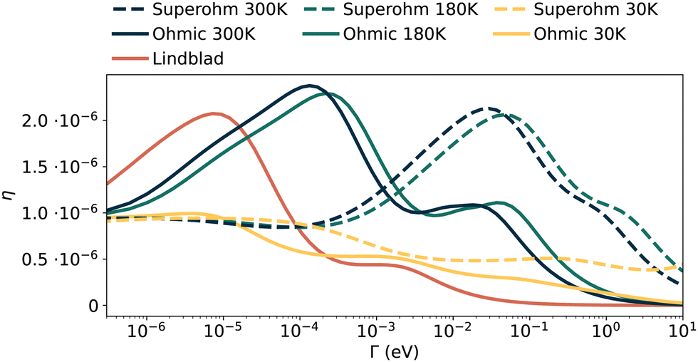 | ||
| Fig. 11 Multi-peaked transport efficiency curves for a single network with uniform on-site energies, showing results from Lindblad pure dephasing, as well as Ohmic and superohmic spectral densities with ωpeak = 0.1 eV. We see similar qualitative behaviour across the Lindblad, 300 K and 180 K curves, with a change in behaviour at 30 K. | ||
As such we can state that these double-peaked effects can and do also occur for these power law spectral densities. However, they occur over a much broader range of environmental couplings, and as such, alternative methods suited to intermediate- and strongly-coupled open quantum systems would be needed to provide more robust statistics.
F Hamiltonian details
Here we list out the data for the specific dipole network presented in Fig. 4 (Tables 2 and 3).| Dipole | X (nm) | Y (nm) | Z (nm) | Energies (eV) |
|---|---|---|---|---|
| 0 (inject) | 0.0 | 0.0 | −10.0 | 1.552794 |
| 1 (extract) | 0.0 | 0.0 | 10.0 | 1.524548 |
| 2 | −5.239018 | −2.013063 | −6.763873 | 1.544986 |
| 3 | −2.429034 | 1.463867 | −2.933762 | 1.552236 |
| 4 | −1.321062 | 4.226071 | −0.255611 | 1.580151 |
| 5 | 3.148822 | −2.374797 | −5.102531 | 1.532472 |
| 6 | −1.552033 | 1.351976 | −1.062326 | 1.560427 |
| 7 | 1.851469 | 1.995554 | 9.06525 | 1.53166 |
| Dipole | d x (e nm) | d y (e nm) | d z (e nm) |
|---|---|---|---|
| 0 | 0.0 | 0.0 | 0.114033 |
| 1 | 0.0 | 0.0 | 0.114033 |
| 2 | −0.054907 | −0.023364 | 0.097174 |
| 3 | 0.016014 | −0.040995 | −0.105197 |
| 4 | −0.065844 | 0.071077 | −0.060133 |
| 5 | 0.02771 | 0.110455 | −0.005934 |
| 6 | 0.081605 | −0.079198 | −0.008472 |
| 7 | 0.058304 | −0.079757 | 0.056948 |
G Reorganisation energies
The goal of this work has been to demonstrate the existence of a new phenomenon in otherwise very typical transport networks. But answering this question is separate from demonstrating if this occurs at typical amounts of coupling to the environment. Also, answering this question cannot be done for the pure dephasing approach used in many studies, and instead requires microscopic couplings to be considered. As such we consider our Bloch-Redfield results in this section, and we calculate the reorganisation energies of our networks in the standard fashion | (11) |
 | ||
| Fig. 12 Bar chart showing what percentage of double-peaked networks have both their peaks below a maximum reorganisation energy of 36 meV. The lower the Drude–Lorentz peak frequency, the more networks meet this criterion. | ||
H Efficiency of single and double peaked networks
Here we consider the maximal efficiency ηmax of the networks in our main data with either a single peak or two peaks. As shown in Fig. 13 we see a very large overlap in the efficiencies shown by either kind of transport efficiency landscape. Suggesting that double-peaked systems can be less efficient, but have such a spread of efficiencies that they are often equally as efficient as the singly peaked systems. | ||
| Fig. 13 Bar chart showing the maximum efficiency ηmax of networks with either a single peak or multiple peaks in their transport efficiency. Y-Axis shows the percentage of each dataset contained within each interval. We see a very strong overlap in the maximal efficiency of either network kind. While double peaked systems can have lower efficiencies, they also have a much larger spread of efficiencies than singly peaked systems. | ||
I Relative efficiency of each peak
We now study the relative efficiency of both peaks in the double peaked case. We define the steady state transport efficiency of the low noise rate and high noise rate peak as ηlow and ηhigh respectively. In Fig. 14 we consider the ratio of these two quantities for our main ensemble of energeticaly disordered networks.
 | ||
| Fig. 14 Histogram of the relative efficiency of systems with multiple ideal noise rates. Peaks at lower noise rates typically have less efficiency than those at higher noise rate. The central two bars contain the majority of systems and correspond to the two peaks having efficiencies within a factor of 2 of each other. | ||
As Fig. 14 shows, the peaks at higher noise rates are typically more efficient than those at lower noise rates. However we also note that for the vast majority of systems the two peaks have efficiencies less than a factor 2 apart. The central two bars of the histogram correspond to the range 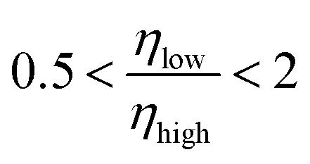 and make up 69.1% of the doubly peaked systems. So in most cases, both peaks have a similar prominence.
J Dense networks
In this work we have considered relatively sparse networks in a volume with a 10 nm radius. This meant there was lots of freedom for the dipoles and their respective exclusion volumes to form many different kinds of structures, while respecting the ideal dipole approximation that we used. However if one wants to understand light-harvesting complexes, these typically occur at higher densities.Here we briefly consider such a dense system, keeping the same model as before with 8 sites, but reduce the full sphere radius to 2.5 nm, close to prior work23 and similarly reduce the exclusion volume around each site to 0.5 nm so that all 6 interior sites can still fit in the volume. The results are shown in Fig. 15, where we see comparable results to those in sparse networks, but with a decrease in the incidence of double peaks at low temperatures.
 | ||
| Fig. 15 Double-peak rates for 1000 dense networks with a volume radius of 2.5 nm and exclusion volume radius of 0.5 nm. We observe no Lindblad peaks in these networks and see the highest rates of double peaks for intermediate temperatures of 180 K. | ||
The reorganisation energies of these peaks were also considered in Fig. 16, where we see that the results at 30 K are consistently the least likely to occur below the cutoff value.
 | ||
| Fig. 16 The percentage of double-peaked dense networks, where both peaks occur below the cutoff reorganisation energy of 36 meV. | ||
K Analysing data
In this work we have used both the Lindblad and non-secular Redfield master equations. By its mathematical construction the Lindblad master equation always produces completely positive density matrices which preserve the trace. Redfield master equations are also linearly trace preserving but can produce unphysical density matrices with negative probabilities.48,61 As this work is looking for peaks in arrays of values, we need to screen these erroneous points as sudden spikes or dips on the otherwise smoothly varying data produce false peaks.To ensure the steady state populations were physical we checked if the trace was unitary and if all the on-site populations were positive. To ensure the steady states were valid we recorded the eigenvalues of each Redfield tensor steady state and then checked their eigenvalues were all between 0 and 1. Tolerances of 10−5 were used for the site checks, and 10−4 for the eigenvalue checks as these were sufficient to remove erroneous points. The points excluded occurred at higher system-environment couplings, while results at lower couplings were rarely if ever excluded. These checks were also applied to the Lindblad results for consistency. With these points removed, simple peak finding algorithms were applied to the remaining valid points in each array: no requirements were placed on the peak prominence, heights or widths.
Acknowledgements
This work was supported by EPSRC Grant No. EP/L015110/1, EP/T007214/1, EP/T01377X/1, and EP/T014032. Calculations carried out in QuTiP,57 data analysis carried out with pandas DataFrames.58,59Notes and references
- S. Kundu and A. Patra, Chem. Rev., 2017, 117, 712–757 CrossRef CAS PubMed.
- I. Kassal, J. Yuen-Zhou and S. Rahimi-Keshari, J. Phys. Chem. Lett., 2013, 4, 362–367 CrossRef CAS PubMed.
- K. Amarnath, D. I. G. Bennett, A. R. Schneider and G. R. Fleming, Proc. Natl. Acad. Sci. U. S. A., 2016, 113, 1156–1161 CrossRef CAS PubMed.
- D. I. G. Bennett, K. Amarnath and G. R. Fleming, J. Am. Chem. Soc., 2013, 135, 1–16 CrossRef PubMed.
- N. C. Chávez, F. Mattiotti, J. A. Méndez-Bermúdez, F. Borgonovi and G. L. Celardo, Phys. Rev. Lett., 2021, 126, 1–25 CrossRef PubMed.
- T. Brixner, R. Hildner, J. Köhler, C. Lambert and F. Würthner, Adv. Energy Mater., 2017, 7, 1–33 Search PubMed.
- F. C. Spano, J. R. Kuklinski and S. Mukamel, J. Chem. Phys., 1991, 94, 7534–7544 CrossRef CAS.
- S. K. Saikin, A. Eisfeld, S. Valleau and A. Aspuru-Guzik, Nanophotonics, 2013, 2, 21–38 CAS.
- M. B. Plenio and S. F. Huelga, New J. Phys., 2008, 10, 113019 CrossRef.
- F. Caruso, A. W. Chin, A. Datta, S. F. Huelga and M. B. Plenio, J. Chem. Phys., 2009, 131, 105106 CrossRef.
- J. Cao and R. J. Silbey, J. Phys. Chem. A, 2009, 113, 13825–13838 CrossRef CAS PubMed.
- M. Mohseni, P. Rebentrost, S. Lloyd and A. Aspuru-Guzik, J. Chem. Phys., 2008, 129, 174106 CrossRef PubMed.
- S. Huelga and M. Plenio, Contemp. Phys., 2013, 54, 181–207 CrossRef CAS.
- I. Kassal and A. Aspuru-Guzik, New J. Phys., 2012, 14, 053041 CrossRef.
- F. Caruso, New J. Phys., 2014, 16, 055015 CrossRef.
- A. R. Coates, B. W. Lovett and E. M. Gauger, New J. Phys., 2021, 23, 1–20 CrossRef.
- A. W. Chin, A. Datta, F. Caruso, S. F. Huelga and M. B. Plenio, New J. Phys., 2010, 12, 065002 CrossRef.
- E. Zerah-Harush and Y. Dubi, Phys. Rev. Res., 2020, 2, 23294 CrossRef CAS.
- A. Olaya-Castro, C. F. Lee, F. F. Olsen and N. F. Johnson, Phys. Rev. B: Condens. Matter Mater. Phys., 2008, 78, 1–7 CrossRef.
- M. Mohseni, A. Shabani, S. Lloyd and H. Rabitz, J. Chem. Phys., 2014, 140, 035102 CrossRef CAS PubMed.
- N. C. Harris, G. R. Steinbrecher, M. Prabhu, Y. Lahini, J. Mower, D. Bunandar, C. Chen, F. N. Wong, T. Baehr-Jones, M. Hochberg, S. Lloyd and D. Englund, Nat. Photonics, 2017, 11, 447–452 CrossRef CAS.
- A. Shabani, M. Mohseni, H. Rabitz and S. Lloyd, Phys. Rev. E: Stat., Nonlinear, Soft Matter Phys., 2012, 86, 11915 CrossRef CAS PubMed.
- G. C. Knee, P. Rowe, L. D. Smith, A. Troisi and A. Datta, J. Phys. Chem. Lett., 2017, 8, 2328–2333 CrossRef CAS PubMed.
- T. Scholak, F. De Melo, T. Wellens, F. Mintert and A. Buchleitner, Phys. Rev. E: Stat., Nonlinear, Soft Matter Phys., 2011, 83, 021912 CrossRef PubMed.
- S. Davidson, F. A. Pollock and E. Gauger, Phys. Rev. Res., 2021, 3, L032001 CrossRef CAS.
- C. Olbrich, J. Strümpfer, K. Schulten and U. Kleinekathöfer, J. Phys. Chem. Lett., 2011, 2, 1771–1776 CrossRef CAS PubMed.
- S. I. Vulto, M. A. De Baat, R. J. Louwe, H. P. Permentier, T. Neef, M. Miller, H. Van Amerongen and T. J. Aartsma, J. Phys. Chem. B, 1998, 102, 9577–9582 CrossRef CAS.
- G. S. Engel, T. R. Calhoun, E. L. Read, T.-K. K. Ahn, T. Mancal, Y.-C. C. Cheng, R. E. Blankenship and G. R. Fleming, Nature, 2007, 446, 782–786 CrossRef CAS PubMed.
- G. Panitchayangkoon, D. V. Voronine, D. Abramavicius, J. R. Caram, N. H. C. Lewis, S. Mukamel and G. S. Engel, Proc. Natl. Acad. Sci. U. S. A., 2011, 108, 20908–20912 CrossRef CAS PubMed.
- S. Davidson, A. Fruchtman, F. A. Pollock and E. M. Gauger, J. Chem. Phys., 2020, 153, 1–16 Search PubMed.
- C. Maier, T. Brydges, P. Jurcevic, N. Trautmann, C. Hempel, B. P. Lanyon, P. Hauke, R. Blatt and C. F. Roos, Phys. Rev. Lett., 2019, 122, 1–8 CrossRef PubMed.
- G. L. Celardo, R. Kaiser and F. Borgonovi, Phys. Rev. B, 2016, 94, 1–12 CrossRef.
- C. M. Kropf, A. Valli, P. Franceschini, G. L. Celardo, M. Capone, C. Giannetti and F. Borgonovi, Phys. Rev. B, 2019, 100, 035126 CrossRef CAS.
- M. Mohseni, A. Shabani, S. Lloyd, Y. Omar and H. Rabitz, J. Chem. Phys., 2013, 138, 204309 CrossRef CAS PubMed.
- Y. Li, F. Caruso, E. Gauger and S. C. Benjamin, New J. Phys., 2015, 17, 13057 Search PubMed.
- M. Walschaers, F. Schlawin, T. Wellens and A. Buchleitner, Ann. Rev. Condens. Matter Phys., 2016, 7, 223–248 CrossRef.
- E. Zerah-Harush and Y. Dubi, J. Phys. Chem. Lett., 2018, 9, 1689–1695 CrossRef CAS PubMed.
- E. Z. Harush and Y. Dubi, Sci. Adv., 2021, 7, 1–9 Search PubMed.
- M. Walschaers, J. F.-D.-C. Diaz, R. Mulet and A. Buchleitner, Phys. Rev. Lett., 2013, 111, 180601 CrossRef PubMed.
- J. Adolphs and T. Renger, Biophys. J., 2006, 91, 2778–2797 CrossRef CAS PubMed.
- M. Schmidt Am Busch, F. Müh, M. El-Amine Madjet and T. Renger, J. Phys. Chem. Lett., 2011, 2, 93–98 CrossRef CAS PubMed.
- M. Wendling, M. A. Przyjalgowski, D. Gülen, S. I. Vulto, T. J. Aartsma, R. Van Grondelle and H. Van Amerongen, Photosynth. Res., 2002, 71, 99–123 CrossRef CAS PubMed.
- B. P. Krueger, G. D. Scholes and G. R. Fleming, J. Phys. Chem. B, 1998, 102, 5378–5386 CrossRef CAS.
- R. E. Blankenship, Molecular Mechanisms of Photosynthesis, Wiley, 2002 Search PubMed.
- A. Ishizaki and G. R. Fleming, J. Chem. Phys., 2009, 130, 234111 CrossRef PubMed.
- J. Moix, J. Wu, P. Huo, D. Coker and J. Cao, J. Phys. Chem. Lett., 2011, 2, 3045–3052 CrossRef CAS.
- H. P. Breuer and F. Petruccione, The Theory of Open Quantum Systems, Oxford University Press, 2007, vol. 9780199213, pp. 1–656 Search PubMed.
- J. Jeske, D. J. Ing, M. B. Plenio, S. F. Huelga and J. H. Cole, J. Chem. Phys., 2015, 142, 064104 CrossRef PubMed.
- F. Fassioli, A. Olaya-Castro and G. D. Scholes, J. Phys. Chem. Lett., 2012, 3, 3136–3142 CrossRef CAS PubMed.
- C. Kreisbeck, T. Kramer and A. Aspuru-Guzik, J. Chem. Theory Comput., 2014, 10, 4045–4054 CrossRef CAS PubMed.
- G. Lindblad, Commun. Math. Phys., 1976, 48, 119–130 CrossRef.
- V. Gorini, A. Kossakowski and E. C. Sudarshan, J. Math. Phys., 2008, 17, 821 CrossRef.
- Y. Dubi, J. Phys. Chem. C, 2015, 119, 25252–25259 CrossRef CAS.
- P. Brumer, J. Phys. Chem. Lett., 2018, 9, 2946–2955 CrossRef CAS PubMed.
- S. Axelrod and P. Brumer, J. Chem. Phys., 2018, 149, 114104 CrossRef PubMed.
- S. Mostarda, F. Levi, D. Prada-Gracia, F. Mintert and F. Rao, Nat. Commun., 2013, 4, 2296 CrossRef PubMed.
- J. R. Johansson, P. D. Nation and F. Nori, Comput. Phys. Commun., 2013, 184, 1234–1240 CrossRef CAS.
- W. McKinney, Proceedings of the 9th Python in Science Conference, 2010, pp. 56–61 Search PubMed.
- The pandas development team, 2021.
- S. Saito, M. Higashi and G. R. Fleming, J. Phys. Chem. B, 2019, 123, 9762–9772 CrossRef CAS PubMed.
- P. R. Eastham, P. Kirton, H. M. Cammack, B. W. Lovett and J. Keeling, Phys. Rev. A, 2016, 94, 1–9 CrossRef.
| This journal is © the Owner Societies 2023 |