 Open Access Article
 This Open Access Article is licensed under a
 Creative Commons Attribution 3.0 Unported Licence
Quantitative studies of crystal nucleation at constant supersaturation: experimental data and models
Richard P.
Sear
*
Department of Physics, University of Surrey, Guildford, Surrey GU2 7XH, UK. E-mail: r.sear@surrey.ac.uk; Tel: +44 (0)1483 686793
First published on 27th May 2014
Abstract
Crystallisation starts off with nucleation, which is rather poorly understood. However, over the last few years there have been important quantitative experiments at constant supersaturation, and the modelling of this data has also advanced. Experiments in which the supersaturation is varying, e.g., those at constant cooling rate, are important but hard to interpret. This review focuses on the state of the art in quantitative studies of nucleation at constant supersaturation. We can now test reliably for heterogeneous nucleation and somewhat less reliably for the rarer case of homogeneous nucleation. In the case of heterogeneous nucleation, we can also obtain at least some information on what is responsible for nucleation. We also now have (unfortunately currently untested) predictions for the scaling of nucleation timescales with system size. These predictions may prove important both for scaling up from small droplets to larger volumes, and for scaling down to crystallisation at the nanoscales relevant for nanotechnology applications. Finally, it is worth noting that in many experiments the dynamic range of nucleation times is too large to be measured. This is presumably due to highly variable impurities, and this problem may need to be addressed in future work.
1. Introduction
Crystallisation lies at the heart of many natural phenomena, and of many technologically important processes. Our climate is affected by clouds of ice particles, and most pharmaceuticals are crystalline. Crystallisation starts with nucleation. Nucleation is the dynamic process that determines how difficult it is for a crystal to form in the system. Here I will only review studies at constant supersaturation, because studies with varying supersaturation are much harder to interpret and to model. At constant supersaturation, nucleation is the process that determines how long you have to wait before a crystal appears in the system. As an example, this waiting time is approximately 160![[thin space (1/6-em)]](https://www.rsc.org/images/entities/char_2009.gif) 000 simulation cycles in the system of Fig. 1.
000 simulation cycles in the system of Fig. 1.
 | ||
| Fig. 1 Plot of homogeneous nucleation occurring in a liquid, in a computer simulation of a simple model. The model is the Gaussian Core model.1,2 In the liquid phase, at each point in time, there are microscopic crystallites formed by thermal fluctuations. The figure shows the number of molecules in the largest crystallite as a function of time. Time is given in Monte Carlo simulation cycles. A cycle is one attempted move per molecule of the liquid. The size of the largest crystallite fluctuates with time, until an unusually large fluctuation takes the crystallite over the nucleation barrier. This occurs at around 160000 cycles. After this the crystal grows rapidly and irreversibly, as seen by the steep increase in size after about 160000 cycles. A snapshot is shown of the growing cluster when it has approximately 500 molecules. Figure courtesy of James Mithen. | ||
In practice there is some ambiguity as to how big this crystal has to be. In experiments the nucleation time is approximated by the time the crystal is first observed, tOBS. This observation is typically via optical microscopy, and is when the crystal is at least many micrometres across. The time to nucleate is probably best defined as the time for the crystal nucleus to reach the (nanoscale) size such that the probability that it will redissolve is negligible, tN. Then if the time for a nucleus this size to grow to be large enough to be observed, tG ≪ tN, tOBS will be a good approximation to a well-defined nucleation time tN. In computer simulations we can observe tN itself, it is about 160000 simulation cycles in Fig. 1.
The study of nucleation at constant supersaturation is essentially the attempt to measure, understand and predict the waiting time before the crystal appears. Ultimately, we want to understand and be able to predict whether the nucleation time will be seconds, minutes, hours, days, years, or too long to be measured. Once nucleation in a system at constant supersaturation is quantitatively understood and modelled then predicting how nucleation occurs at varying supersaturation (e.g., varying temperature) should be possible.
Although control over crystal growth is also important, nucleation can probably define which polymorphs can form, and can set both the lattice orientation2 and the size of the crystals produced. Too fast nucleation can produce a shower of small crystals when perhaps a single crystal is desired. However, if nucleation is slower than the experimental timescale then crystallisation will be prevented altogether.
There is considerable evidence that nucleation is a stochastic process, i.e., there is randomness inherent in it. In the computer simulation of simple systems this is clearly true. If the simulation of Fig. 1 was rerun the waiting time before nucleation would not be the same. It could be 20000 simulation cycles, 300000 cycles, etc.
In molecular, ionic and metal systems, nucleation occurs on time and length scales that are inaccessible to conventional experiments: the nucleus is only briefly at the top of the barrier and is then only a few molecules (and hence nm) across. The nucleus in Fig. 1 is of a few hundred molecules, and if we convert from simulation to experimental time units, then it spends only nanoseconds near the top of the nucleation barrier. Also, the nucleation of a crystal is almost always heterogeneous, i.e., it occurs on a surface in contact with the fluid. Typically this is the poorly characterised surface of an impurity. This is well established for the best studied system: ice nucleation.3,4 For all these reasons, despite its importance nucleation is poorly understood.
The structure of this review is as follows. The next section introduces isothermal nucleation. The heart of this review is sections 3 and 5. Section 3 reviews quantitative experimental data on isothermal nucleation, and section 5 reviews the models that have been fitted to this data. In between these sections we briefly cover the classical theory of nucleation.
Then there a few short sections highlighting particular features of the data or approaches to modelling it. This starts with section 6, which points out that there are many results from the field of survival data analysis5,6 that may be useful in the study of nucleation. Section 7 covers the important problem of how nucleation times scale with volume, and section 8 highlights the common observation that the spread of nucleation rates is often so large that it exceeds the dynamic range of the experiment. The final section is a conclusion and consideration of future work.
2. Introduction to nucleation at constant supersaturation
The cleanest and so easiest to interpret experimental data on the nucleation of crystals is that on small droplets at constant supersaturation. We refer to this as isothermal crystallisation, because to keep the supersaturation constant the temperature must be kept constant. The pressure, and in the case of solutions, the concentration must also be kept constant. If the supersaturation is varying with time then this will cause any free energy barriers to nucleation to also vary with time, greatly complicating analysis of the data.Small droplets mean that only one nucleation event is needed for crystallisation, and the crystal that results from this event can easily be observed. To accurately measure a nucleation time, the time for the nucleus to grow large enough to be observable, tG, should be short, in comparison to the nucleation time, tN. For example, the time for a single microscopic nucleus to grow to freeze all of a small water droplet, may be of order seconds or less. Then we can measure the crystallisation time and this will provide a good approximation for the time for nucleation (the time we are interested in), provided this nucleation time is at least around 10 minutes or more.
2.1. P(t) plots
A useful way to plot isothermal nucleation data is to plot the cumulative probability P that nucleation has not occurred as a function of time t. In experiment this is straightforward to obtain. Some large number, perhaps 50 or more, nominally identical droplets are prepared, and then followed over time. The fraction of droplets in which nucleation has not occurred is then an approximation to P(t). The probability density that nucleation occurs at a time t, p(t), is related to P(t) by p(t) = −dP(t)/dt. It is in general probably better to work with P(t) rather than p(t), because p(t) will be noisier.We can also define an effective nucleation rate as a function of time, h(t), via the differential equation
 | (1) |
If the effective nucleation rate is constant, h(t) = k. Then the solution to eqn (1) is the simple exponential
| P(t) = exp[−kt] exponential | (2) |
We show the results of nucleation in a simple lattice model (the lattice gas or Ising model) in Fig. 2. This is heterogeneous nucleation, nucleation is occurring at a surface. The result for nucleation at a surface that is not changing with time is shown as the purple curve in Fig. 2. The curve is well fit by a simple exponential: P(t) = exp[−1.22 × 10⁻⁶t], so here the nucleation rate is k = 1.22 × 10⁻⁶ per cycle (time here is in units of simulation cycles).
 | ||
| Fig. 2 Plot of the probability that nucleation has not occurred, P(t), as a function of time, t, for computer simulation of nucleation in a simple lattice model.7 Time is in units of computer simulation cycles. The solid purple curve is at a supersaturation of 2h/kT = 0.16, and is for nucleation on a surface that is not changing with time (rD = 0). The magenta dotted curve is a fit of an exponential function to this P(t). The solid black and green curves are for nucleation on surfaces that are changing with time. The surfaces are slowly dissolving, at rates rD = 10−6 and rD = 2 × 10⁻⁶, respectively. In both cases, the supersaturation is lower than for the purple curve at 2h/kT = 0.12. The brown and turquoise dotted curves are fits of the function of eqn (11) to the black and green P(t)'s respectively. In all cases the simulation P(t)'s are obtained from 250 nucleation runs. From ref. 7. Copyright 2014 Sear. Distributed under Creative Commons Attribution 3.0 license. | ||
An exponential decay of P(t) is expected whenever there is a well-defined and time independent nucleation rate. Thus when we review experimental P(t) data below, when we see a simple exponential P(t) we state that this data provides evidence for a well defined nucleation rate. We call this class I nucleation. As in class I nucleation P(t) is exponential, lnP(t) is a straight line, of slope −k, and the effective rate h(t) is a constant.
We use P(t) and h(t) to define two more classes of nucleation, class II and class III. Class II is where the effective rate h(t) is a decreasing function of time, dh/dt < 0. Then lnP(t) curves upwards. Class III is the opposite case, where the effective nucleation rate is an increasing function of time dh/dt > 0. Then lnP(t) curves downwards. All three classes are seen in experiment and will be reviewed here.
3. Experimental results on the isothermal nucleation of crystals
In this section we review experimental results for P(t) for the isothermal nucleation of the crystal phase in small droplets or in small volumes in vials. We will mention some models, but the models themselves are reviewed in the next two sections. In this section, the work reviewed is divided up according to the class (I, II or III) of P(t) found. We start with the simplest class, class I where P(t) is a simple exponential.3.1. Class I: exponential P(t)
The 2004 paper of Duft and Leisner8 is a particularly clear example of a system where there is evidence for a nucleation rate that is well defined, and where in addition this rate is proportional to the volume. If we look at Fig. 3 we see that if an initial transient due to temperature-equilibration is excluded, the plot of lnP(t) is a straight line. Thus, P(t) is a simple exponential. Also, the slope of lnP as a function of time is 16.5 ± 0.6 times larger for the large droplets than for the small droplets. The ratio of the volumes of the two droplets is 17.2 ± 0.8, and so the data is consistent with a nucleation rate that scales as the volume. The rate per unit volume is of order 1012 m−3 s−1, or 10−24 nm−3 ns−1.
 | ||
| Fig. 3 Plot of the logarithm of the fraction of unfrozen water droplets, Nu(t)/N0, as a function of time. The plot is from Duft and Leisner,8 and is for the freezing of water droplets to form ice at T = 237.1 K. The green circles are for droplets of radius 49 μm, and the purple squares are for smaller droplets of radius 19 μm. Copyright 2004 Duft and Leisner. Distributed under Creative Commons Attribution 3.0 license. | ||
As Duft and Leisner state, this provides good evidence that the nucleation is actually homogeneous nucleation. Note that this is at the low temperature of T = 237.1 K (−36 °C). At higher temperatures water freezes via heterogeneous nucleation.3 However, note that even here, this behaviour is also consistent with nucleation on microscopic impurities which are present in the water at a fixed concentration, and where the spread of nucleation barriers is small.10
But if we assume that indeed this is homogeneous nucleation, then a rate per unit volume of order 10−24 nm−3 ns−1 implies a free energy barrier to homogeneous nucleation of around kT ln(1024) = 55kT. This assumes a molecular volume of 1 nm3 and a molecular timescale of 1 ns. So even though nucleation is rapid here (within seconds, see Fig. 3) there is a still a substantial free-energy barrier.
The work of Duft and Leisner8 is a good example of how to use quantitative experimental data to provide evidence that nucleation occurs according to the standard classical nucleation theory picture for homogeneous nucleation. They show both that a rate is well defined and time independent (as P(t) is exponential), and that it is proportional to the volume, as a homogeneous nucleation rate should be. This is obviously superior to just asserting that nucleation is homogeneous, without providing evidence, which a number of other authors do. It should be noted that this work is far from the first work to see a clean exponential dependence for P(t). For example, in 1974 Miyazawa and Pound11 found similar behaviour for the crystallisation of liquid gallium.
Massa and Dalnoki-Veress12 also found exponentially decaying P(t) curves, with slopes that scaled approximately with volume. This was for the nucleation of the crystal phase in droplets of the polymer poly(ethylene oxide) (PEO). Again this data is consistent with homogeneous nucleation.
The second study I wish to discuss in detail is by Carvalho and Dalnoki-Veress,9 who studied the crystallisation of small (of order 10 μm across) PEO droplets on three different polystyrene (PS) substrates. Results for P(t) are shown in Fig. 4. They also studied the crystallisation of polyethylene.13 In most cases lnP(t) is, to a reasonable approximation, a straight line, indicating a well-defined and time-independent nucleation rate. Note that these plots are all for only a subset of the droplets studied. In each experiment some droplets crystallised on cooling from high temperatures to the temperature studied in that experiment, and some crystallised in the first 400 s of the experiment. All these droplets were discarded. Thus the complete sets of droplets do not have a well-defined nucleation rate, presumably due to some of them having impurities that are very active at inducing nucleation. However, for a subset of the droplets it is possible to define a nucleation rate, via the plots in Fig. 4.
 | ||
| Fig. 4 (a)–(c) The logarithm of the fraction of droplets not crystallised, Na(t)/N0, as a function of time t. The droplets are of the polymer polyethylene oxide (PEO), and they are on polystyrene (PS) substrates. This is the work of Carvalho and Dalnoki-Veress.9 The different curves in each plot are for droplets of different sizes, as measured by the areas of the substrate the PEO droplets cover. These areas are given in the keys of (a)–(c). (a) Droplets of PEO on smooth amorphous PS (T = −2 °C). (b) PEO on a rough crystalline PS substrate (T = 4 °C). (c) PEO on an even rougher crystalline PS substrate (T = 10 °C). The crystalline substrates are annealed at different temperatures, (b) at 185° and (c) at 175 °C, to create the different roughness. The variation in nucleation timescale τ with droplet radius R is plotted in (d). The timescale τ = one over the slope of ln(Na(t)/N). The nucleation timescale varies approximately as one over the droplet volume (n = 2.9) for droplets on the smooth substrate, as one over the droplet area (n = 2.1) on the rough crystalline substrate, and as one over the radius (n = 1.0) on the even rougher substrate. Copyright 2010 by The American Physical Society. | ||
For PEO droplets on a smooth PS substrate, this nucleation rate was found to scale as the volume of droplets. The scaling is shown in Fig. 4(d). It is consistent with homogeneous nucleation and is just what Duft and Leisner8 found for ice (Fig. 3). On two different rougher PS substrates, Carvalho and Dalnoki-Veress9 found nucleation rates that scaled as droplet area in one case, and droplet linear dimension in the other. This is shown in Fig. 4(d). The scaling with area was found for the less rough of the two rough PS surfaces. A nucleation rate that scales as droplet area is consistent with nucleation on a reasonably homogeneous interface. As the only interface that changes between the data of Fig. 4(a) and (b) is the PS/PEO interface, this suggests that the PEO crystals in (b) are nucleating at the interface between the liquid PEO and the rough PS substrate.
On a PS substrate with a larger roughness, the rate scales with the linear size of the droplet. This is the behaviour expected when nucleation occurs on something that is proportional to the diameter of the droplet. The obvious object with size proportional to the diameter is the contact line at the edge of the droplet where the PEO/air interface meets the PEO/PS interface. Studies of the final crystallised droplets via atomic force microscopy (AFM) are consistent with this idea. AFM images of crystallised PEO droplets are shown in Fig. 5. It appears (Fig. 5b) and c)) that on the roughest substrate the droplets started to crystallise from a point on their edge.
 | ||
| Fig. 5 AFM images of crystallised PEO droplets on PS substrates, from Carvalho and Dalnoki-Veress.9 The droplets are about 8 μm across. (a) is a droplet on a smooth amorphous PS substrate. (b) and (c) are droplets on the rougher of the two crystalline substrates. The arrows indicate assumed nucleation sites, which are at the edges of the droplets for (b) and (c). Copyright 2010 by The American Physical Society. | ||
It is not known why on the rougher substrates, the droplets should crystallise at the contact line. The nucleation barrier can be lower at a contact line than at an interface,14,15 but it is not clear how changing the substrate roughness will affect this. The nucleation of ice has been studied at contact lines where the air/water interface hits a solid surface. However, mixed results have been found in the sense that some studies find nucleation preferentially at the contact line,16 while other studies do not.17,18 See Gurganus et al.18 and my earlier review15 for discussion of this point.
Finally, both Jiang and ter Horst,20 and Quon et al.21 also found approximately exponential P(t)'s. In the case of Jiang and ter Horst this needed a small time offset, to account for growth. The results of Jiang and ter Horst,20 and Quon et al.21 are also consistent with well defined nucleation rates that are in the thermodynamic limit. Jiang and ter Horst's20 data is on the crystallisation from solution of the molecules m-aminobenzoic acid (m-ABA) and L-histidine (L-His), while Quon et al.'s21 is for crystallisation of the drug paracetamol (also called acetaminophen).
3.2. Class II: decreasing effective nucleation rate
Our first example of a system with a decreasing effective rate, h(t), is shown in Fig. 6. This is the work of Diao et al.19 on the nucleation of crystals of aspirin from solution. Diao and coworkers have also studied other systems, such as the molecules ROY and paracetamol, and also found results where the effective rate is a decreasing function of time.22–24 | ||
| Fig. 6 Plots of the probability P that nucleation has not occurred in a droplet, as a function of time. This is the work of Diao et al.,19 and is for the nucleation of aspirin from solution. The solvent is a mixture of water and ethanol. The supersaturation is 2.1. Polymer microgel particles are added to the solution in all three cases. The polymer is poly(ethylene)glycol diacrylate (PEGDA), made with PEG of varying molecular weights: 200, 400 and 700 g mol−1. The microgel particles were added to induce nucleation. The curves are fits of the Weibull function, eqn (3), to the data. The values of β are 0.52, 0.69 and 0.36 for polymer made with PEG molecular weights of 200, 400 and 700 g mol−1, respectively. Reprinted with permission from ref. 19. Copyright 2012 American Chemical Society. | ||
In most of the work reviewed here, nucleation is presumably occurring on either impurities in the solution or at a surface in contact with the solution. The work of Diao et al.19 is an exception. They deliberately added particles of a hydrogel to their solutions to induce nucleation. Material added to provide surfaces for nucleation is sometimes called a nucleant.26–28 Nucleants are particularly common in protein26–28 and ice crystallisation.4,25,29–32 Often the surfaces of the nucleants are both disordered and poorly characterised, i.e., we know little more about them than we do about any impurities that might be present. However, progress is being made at characterising these surfaces,28,30–33 and here at least we have a good idea what nucleation is occurring on. So nucleants are a promising way to improve our understanding of the mechanism of nucleation.
If we focus on the data plotted in red, we see that around 20% of the samples crystallise inside around 50 min but that almost 40% of the samples have still not crystallised after almost 1400 minutes. Thus the nucleation times span two orders of magnitude and more. This is very different from nucleation at a constant rate where P(t) is exponential and the standard deviation of nucleation times is equal to the mean. Here as not all the samples crystallised we cannot even calculate the standard deviation or mean of the nucleation time. This implies that work that does not report a P(t) but does report both a mean nucleation time and a standard deviation, would be inconsistent with a well-defined constant rate if the ratio standard-deviation/mean is significantly different from one.
Diao et al.19 fitted a function called a Weibull function to their data. The Weibull function is
| P(t) = exp[−(t/τ)β] Weibull | (3) |
It is the exponential of a power law, with exponent β. The parameter τ is a timescale that is related to the median nucleation time, tMED, by τ = tMED(ln2)1/β. The Weibull function is a two-parameter cumulative distribution function. For β = 1 it reduces to a simple exponential. For a Weibull, the effective nucleation rate h(t) = βtβ−1/τβ. For β < 1, the effective rate h(t) decreases monotonically with time, so then nucleation is class II, while if β > 1, h(t) increases with time, so then nucleation is class III.
The best fit values for β found by Diao et al.19 were all less than one, so their data is in class II. It is worth noting that when β < 1, the Weibull function is also known by other names. It is often called a stretched exponential.34 Also in the study of glassy behaviour it is sometimes called a Kohlrausch or Kohlrausch–Williams–Watts function. When β > 1 the Weibull function is also called a compressed exponential.
Not all Diao et al.'s19 data was well fit by a stretched exponential, some was better fit by the sum of two exponentials. As a sum of two exponentials has three parameters, one more than the Weibull has, this is however not a fair comparison. But it may well be that in some of their data there are two types of droplet, each with a well defined but different rate, and then P(t) will genuinely be the sum of two exponentials. A sum of two exponentials is always in class II.35 Earlier work by Kabath et al.36 on the nucleation of ice, also found two slopes and hence possibly two rates.
Although the work of Duft and Leisner8 on the nucleation of ice (Fig. 3) found a well-defined nucleation rate, other work on ice nucleation25,37 has found a rate that decreases with time. Both Welti et al.37 and Herbert et al.25 found that they could fit their data reasonably well with models that include quenched disorder. Results from Herbert et al.25 are shown in Fig. 7. We see that lnfliquid(t) = lnP(t) is far from a straight line. It curves upwards. In this work the mineral potassium-feldspar was added to the water droplets to induce nucleation. This mineral is common in the atmosphere and affects ice nucleation there. Instead of fitting this curve directly they fitted to data obtained at a constant cooling rate, over a temperature range of 4 K that includes the temperature of this experiment. The model used includes quenched disorder, and we see that it predicts the time dependence of P(t). This model relates nucleation data at constant cooling rate to isothermal data.
 | ||
| Fig. 7 Plot of the logarithm of the fraction of a set of water droplets that are still liquid, fliquid, as a function of time. This is the work of Herbert et al.25 The water droplets contain the mineral potassium-feldspar added to induce nucleation. The right-hand axis shows the actual number of droplets of water that are still liquid. This is at a temperature of 262.15 K. The experimental data is shown by the red triangles. The dashed curve is the prediction of a model fit to data at constant cooling rate, between approximately 260 and 265 K. This model incorporates a spread of nucleation rates between the droplets (quenched disorder). The solid curves are predictions of a model that assumes that the rate is the same in all droplets, and so that fliquid decays exponentially. The two solid curves are obtained for data at two different constant cooling rates, 0.2 and 2 K min−1. The shaded areas indicate the uncertainty in predicted fliquid curve due to uncertainty in the measured temperature. Copyright 2014 Herbert et al. Distributed under Creative Commons Attribution 3.0 license. | ||
Knezic et al.38 also found a P(t) with an effective nucleation rate that was decreasing with time. This was for the crystallisation of the protein lysozyme from solution, in levitated droplets. Their data is shown in Fig. 8. They also found that a Weibull function with β < 1 provided a reasonable fit to the data. Their best fit value for β was β = 0.6. This work, in 2004, is the earliest work I am aware of that fitted P(t) data with a Weibull function.
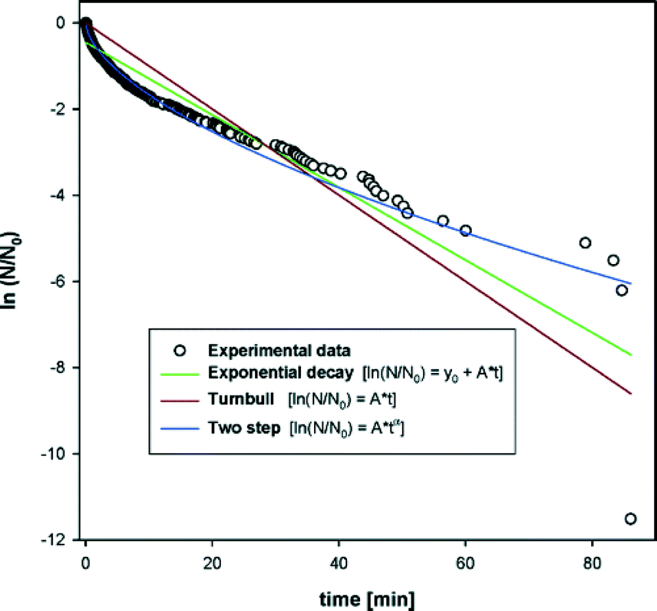 | ||
| Fig. 8 Plot of the logarithm of the fraction of droplets that have not crystallised, as a function of time. This is the work of Knezic et al.,38 and is for the nucleation of the protein lysozyme in solution. Three fits to the data are shown. A simple exponential, eqn (2), which is the brown curve labelled ‘Turnbull’. A simple exponential with a time offset, which is the green curve labelled ‘Exponential decay’. A Weibull function, eqn (3), which is the blue curve labelled ‘Two step’. For this fit, β = 0.6. Reprinted from ref. 38 with permission. Copyright 2004 American Chemical Society. | ||
However Knezic et al. were far from the first to observe an effective nucleation rate that decreased with time. Over 50 years before them, Pound and La Mer39 studied the crystallisation of oxide coated droplets of liquid tin. They also found an effective nucleation rate that was a decreasing function of time. To model this, they developed the Pound–La Mer model for P(t). We will discuss this model in the model section.
The Pound–La Mer model was also used by Laval et. al.40 They used it to fit data on the crystallisation of potassium nitrate from aqueous solution. The results of Laval et al. are shown in Fig. 9. Also Teychené and Biscans41 used the model to fit data on the crystallisation of elfucimibe from octanol solution. Elfucimibe is a pharmaceutical molecule. In both40,41 cases the Pound–La Mer model fits the data well, although it should be noted that as this model has 3 parameters (one more than Weibull and two more than a simple exponential) we should expect it to fit well.
 | ||
| Fig. 9 Plots of (a), the probability P, and (b), lnP, both as a function of time. This is the work of Laval et al.,40 and is for the nucleation of potassium nitrate crystals in water, at a concentration of 40 g of potassium nitrate added to 100 g of water. From top to bottom the curves are at temperatures 3.8, 2.8, 1.9, and 0.9 °C. The solubility of potassium nitrate decreases with decreasing temperature so the lower the temperature the higher the supersaturation. The fits to the data in (b) are of the Pound–La Mer model, eqn (7). Reprinted from ref. 40 with permission. Copyright 2009 American Chemical Society. | ||
A weakness of P(t) plots is that they do not directly distinguish between what is called thermal disorder, and what is called quenched disorder. Thermal disorder is disorder (which is just another word for randomness here) in the time nucleation occurs in a droplet due to the fact that nucleation is a thermal fluctuation. This is the disorder seen in spread of nucleation times in the simulation data of the purple curve in Fig. 2. Quenched disorder is disorder, i.e., randomness, due to fixed, i.e., time-independent, variability in the impurities present in droplets.
For example, if nucleation occurs in droplet 1 before droplet 2, we do not immediately know if this is because just by chance the nucleation fluctuation occurred earlier in droplet 1 than droplet 2, or if droplet 1 has an impurity particle in it that makes a large contribution to the nucleation rate, but droplet 2 does not. In the second case but not the first the nucleation rate is different in droplets 1 and 2.
A direct way to distinguish between quenched and thermal disorder is to do multiple crystallisation runs on the same set of droplets. To do this, care needs to be taken to test for any significant changes in the droplets when crystallisation occurs, and that after one crystallisation run, the crystals are completely dissolved before the next run. Laval et al.40 did this. They checked that the mean number of crystals found in each cycle did not drift (evidence that the nucleation sites were not being altered by crystallisation and dissolution), and that varying the temperature and time used to dissolve the crystals did not change the results in the next cycle (evidence that the crystals dissolved completely erasing any memory of what occurred in the previous cycle). Their results are in Fig. 10. When the sample is crystallised multiple times the thermal disorder will be different each time but the quenched disorder, by definition, remains the same. Essentially, the barrier stays the same but the time to cross still has random variability, as crossing is a thermal fluctuation. Haymet and coworkers have also studied42 this, for the freezing of water, but they worked at constant cooling rates.
 | ||
| Fig. 10 Results from an experiment by Laval et al.40 to directly observe time-independent droplet-to-droplet variability. The experiments are done on a set of approximately 160 droplets of potassium nitrate solution (produced using microfluidics). Part (a) has two parts. The top part is the temperature profile as a function of time applied to the set of droplets. The temperature is cycled seven times between a high supersaturation maintained for a fixed time to drive crystallisation, and undersaturated conditions to dissolve the crystals before the next cycle. The bottom part of (a) is 6 (14 × 25 mm2) images taken of the set of droplets at the point on the temperature profile indicated by the circle, the diamond, the triangle, etc. Each of these images is taken at the end of the low-temperature part of a single temperature cycle, when nucleation has occurred in about one fifth of the droplets. The image is taken between cross polarisers and so (only) the droplets with crystals appear as bright spots. Images are shown for only 6 of the 7 temperature cycles. Part (b) of the figure is the function pg(nc), the probability that a droplet crystallised exactly nc times in the 7 cycles. The experimental data is shown as the histogram, while the squares joined by lines is the theoretical prediction, eqn (4), in the absence of quenched disorder. Reprinted from ref. 40 with permission. Copyright 2009 American Chemical Society. | ||
Laval et al.40 performed 7 crystallisation runs (by cycling the temperature) on a set of about 160 droplets. On average in a single run a fraction 0.19 of the droplets crystallised. If there is no quenched disorder in the system then all 160 droplets are equivalent and so equally likely to crystallise in any given run. Then the probability that a randomly selected droplet crystallises nc times in total in the 7 experiments is just given by the standard expression from combinatorics
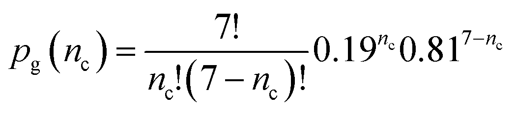 | (4) |
This function is plotted as the solid squares joined by lines in Fig. 10. The experimental data is shown as a histogram. Clearly the prediction assuming no quenched disorder is very far from the experimental data. This large difference rules out the possibility that the droplets are all equivalent. There is quenched disorder present; there is droplet-to-droplet variability that is independent of time, i.e., is present from one temperature cycle to the next.
We can approximately quantify the relative contributions of thermal and quenched disorder as follows. If quenched disorder dominated thermal disorder then a particular droplet would either freeze 0 times or 7 times, i.e., freezing of a droplet would be completely predictable after the end of the first temperature cycle. Here, about 70% of the droplets froze 0 or 7 times, leaving only 30% where thermal disorder apparently played a role. It is worth noting that in the literature on ice nucleation at constant cooling rate, extensive use25,29,31,37,44–47 is made of models which have quenched but no thermal disorder. These are called3 ‘singular’ models.
In other systems cycling the temperature and so repeatedly crystallising and then melting may change the system. I am not aware of any study of the effect of cycling on P(t), but Durant and Shaw48 observed an effect of cycling on the freezing temperature of water droplets. It appears that initially the droplets had small air bubbles inside them. These bubbles affected nucleation, but they were expelled by repeated crystallisation cycles. Further cycles in this system caused particles to move from the bulk of the water droplet to its surface and this also affected nucleation. Any work that cycles the system into and back out of the crystalline state, for example to test for the affects of quenched disorder, will need to carefully check to see if processes similar to those seen by Durant and Shaw are occurring.
In all the experiments we have reviewed so far, crystallisation was observed by direct observation of the crystals formed, using optical microscopy (sometimes with crossed polarisers). For nanoscale droplets, less than the wavelength of light across, direct visual inspection of crystallisation is not possible. However, Schwind et al.43 used the difference in localized surface plasmon resonance (LSPR) signal between the liquid and crystal states, to follow isothermal crystallisation in tin nanodroplets. Their results are shown in Fig. 11.
 | ||
| Fig. 11 Freezing kinetics at four different temperatures, for tin nanoparticles, from the work of Schwind et al.43 The nanoparticles are on a sapphire substrate and are coated with SiO2. They are approximately 100 nm across by 50 nm high.43 Plotted is the normalised difference between the localized surface plasmon resonance (LSPR) signal when all droplets are crystal and the LSPR signal when they are all liquid. Assuming that the droplets contribute independently to the LSPR signal, this is P(t). The data do not fall on simple exponential curves. The data was fitted using a power-law function, 1/(1 + rt)n. The fitted parameter values n and r are as follows: 0.782 and 8.98 × 10⁻⁵ s−1 (100.3 °C); 1.42 and 2.96 × 10⁻⁴ s−1 (97.1 °C); 2.49 and 2.67 × 10⁻⁴ s−1 (95.1 °C); 5.94 and 2.40 × 10⁻⁴ s−1 (94.3 °C). Reprinted from ref. 43 with permission. Copyright 2010 American Chemical Society. | ||
It appears that P(t) is not a simple exponential for these very small crystallising systems. They fit a two-parameter function of the form P(t) = 1/(1 + rt)n (n, r > 0) to their data. This corresponds to an effective nucleation rate as a function of time, h(t) = nr/(1 + rt), which is a decreasing function of time. Thus, to the extent that this function fits the data well, the nucleation here is in class II. Techniques such as LSPR mean that, at least in some systems, we can study nucleation kinetics down to very small droplet sizes.
3.3 Class III: increasing effective nucleation rate
A nucleation rate that increases with time will result in a plot of lnP(t) curving downwards. Examples of this behaviour are rare, but Kim et al.49 find just such behaviour for the crystallisation of the explosive RDX from acetone solution. Their results are shown in Fig. 12. The only other examples I know of are those of Weidinger et al.,50 Toldy et al.51 and Boinovich et al.52 Note that the P(t)'s plotted in Fig. 12 are initially almost horizontal and close to one, indicating very little nucleation, and then curve downwards, dropping more and more steeply as time increases. The effective nucleation rate is a rapidly increasing function of time.
 | ||
| Fig. 12 Plot of the fraction of vials N/N0 (on a logscale) in which nucleation has not occurred, as a function of time. This is the work of Kim et al.,49 and is for the nucleation of RDX crystals from acetone solution, in 3 ml vials. The black squares are data for just RDX in acetone, while the other symbols are data where in addition different molecules were added to affect the nucleation. Solid curves are fits of the Weibull function, eqn (3), to the data, and dashed curves are fits of a simple exponential, eqn (2), to the data. Reprinted from ref. 49 with permission. Copyright 2013 American Chemical Society. | ||
In Fig. 12, Kim et al.49 have fitted both simple exponential functions (dashed curves) and Weibull functions (solid curves). For the Weibull fits, Kim et al.49 obtain best fit values of β that are greater than one, indeed they find values up to ≃5.5. This is true without additives (black squares), with solutephilic polymer molecules added (green diamonds), and with amphiphilic molecules added (the other data points). Thus although the additives do affect the rate they do not affect the qualitative shape of the P(t) curves. It is not known why the additives have this effect. Weidinger et al.50 fitted their data for the freezing of the alkane C15H32 with a function close to a Weibull and used values of 2 and 3, for the equivalent parameter to β.
For β > 1 the effective nucleation rate h(t) is an increasing function of time, so this is class III nucleation. When β > 1 the slope of the Weibull function tends to zero, as t → 0, i.e., there is an initial plateau at short times. We see that this feature is clearly present in the data in Fig. 12. The larger the value of β, the longer the initial plateau, in relation to the time taken for nucleation to occur once P(t) starts to drop. So the large best-fit values of β are due to the long initial plateau followed by a steep drop. We discuss the Weibull function in the models section.
It is worth noting that the Gompertz function (see eqn (10) in the models section) fits the data of Kim et al.49 approximately as well as the Weibull function.53 The Gompertz function has the same number of parameters as the Weibull (two), and it looks qualitatively like the Weibull with β > 1. The Gompertz function can be derived, see section 5.2, from the assumption that the rate is an exponentially increasing function of time.
As Kim et al.49 note, the measured nucleation time is the time to first observe a crystal in the solution, and this will differ from the true nucleation time by tg, the time needed for the nucleated crystal to grow large enough to be visible. Thus it is difficult to rule out some of the width of the initial plateau in P(t) being due to this growth time. It is also possible that some of it may be due to time taken for the sample to equilibrate at the temperature of the experiment, from the higher temperature used to dissolve the RDX. Note that in Fig. 3 there is a short initial plateau that is believed to be due to temperature equilibration.
Thus, due to the nature of the P(t) curves it is harder to demonstrate that there is an increasing nucleation rate than to demonstrate that there is an decreasing nucleation rate. Delays due to the time for crystals to grow large enough to be observed, and due to the time required for temperature equilibration are alternative sources of an initial plateau in P(t) at short times.
Earlier work by Weidinger et al.50 not only also observed an initial plateau in P(t) but they observed changes in the droplet during that plateau, and proposed a plausible mechanism for the plateau. Their work is on the freezing of levitated droplets of the alkane C15H32. Interestingly, they observed changes, probably in the surface of the levitated droplet, prior to nucleation. It is known50,54 that alkanes can undergo surface freezing. Surface freezing is a surface phase transition where surface layers can crystallise before the bulk. Any change at the droplet surface will affect nucleation there.15,54–57
Thus, as Weidinger et al.50 note, it seems possible that here the nucleation rate is low until a surface phase transition occurs, which then greatly increases the nucleation rate. This would be consistent with the class III behaviour observed. Such a mechanism may even be common. In many systems surface phase transitions may go unnoticed, for example if they occur on the surfaces of small impurity particles. This is worth further investigation.
Finally, Toldy et al.51 see similar behaviour to Kim et al.49 and Weidinger et al.50 They studied glycine crystallising in solution, but in the work of Toldy et al. the crystallising droplets may not be independent of each other. They sometimes observe that once one droplet has crystallised, then neighbouring droplets may crystallise. This means droplets are not independent, which can give an effective nucleation rate for the ensemble of droplets that increases with time, even when the rate in an isolated droplet may not be increasing with time. This effect complicates understanding the nucleation behaviour.
4. The classical theory for the nucleation of crystals
The standard theory for the nucleation of crystals is classical nucleation theory.15,55,58 This assumes that nucleation is an activated process where the rate is low because there is a free energy barrier to nucleation F*. By low we mean that the timescale for nucleation can be seconds, hours or more, which is many orders of magnitude larger than the nanosecond timescale for the dynamics of molecules in solution.The classical nucleation theory prediction for the nucleation rate of homogeneous nucleation, RHOM, is given by55,58
| RHOM = MjZ exp(−FH*/kT) | (5) |
I define homogeneous nucleation to be nucleation where the nucleus consists just of the molecules of the new crystal phase and where the nucleus is not in contact with anything. FH* is the free energy change on forming a nucleus at the top of the barrier, in the bulk of the liquid. In eqn (5), M is the number of molecules of the crystallising substance, j is the flux of monomers onto a critical nucleus, and Z is essentially the probability that the critical nucleus goes forward into the new phase not back into the metastable phase.55
If the nucleus is in contact with anything or contains another species that alters the barrier, I call that heterogeneous nucleation. See an earlier review15 for a discussion of the assumptions that are made to derive eqn (5).
But as we have seen, nucleation is rarely homogeneous. Nucleation is usually heterogeneous, it occurs at a surface.15,19,22,55,59,60 This surface may be of a nanoscale object.28,59 These surfaces are often rough and disordered7,19,27,59 and the nucleation rate at a surface is very sensitive to almost all details of local surface chemistry and geometry.15,33,61–64 Thus there will only be a single nucleation barrier at a totally flat smooth edgeless surface. On a rough surface there is not one barrier but many different nucleation barriers. The barrier will be high at points on the surface where it is difficult for the nucleus to form and low at points where it fits well onto the surface.
Thus, within classical nucleation theory, the nucleation rate, RHET, in the presence of rough disordered surfaces is given by27,65
 | (6) |
As the nucleation rate varies exponentially with the barrier at a site, Fi*, it is reasonable to assume that the variation in rate from site to site is dominated by the variation in Fi*, i.e., that we can neglect any variability on ji and Zi. If over the course of the experiment the surface is not changing with time, then the Fi* are fixed.
In practice we are never in a position to calculate the sum in eqn (6). The surfaces nucleation is occurring on are typically very poorly characterised. And without knowledge of the surface geometry and surface chemistry we cannot calculate the Fi*.
However, for disordered surfaces the Fi* should be random variables drawn from an (unknown) probability density function p(F*). We show a schematic of a possible probability density function for the site barriers in Fig. 13. Even without knowing anything about the distribution of nucleation barriers, we can say that there are two qualitatively different possibilities.
 | ||
| Fig. 13 A schematic plot of the log of the probability density p(F*/kT) of free energy barriers to heterogeneous nucleation, F*. The plot is just a simple illustrative probability density, meant to show possible features of a distribution of nucleation barriers. Illustrated is an effectively delta-function peak at large barriers for nucleation at a free liquid surface, a broader peak at lower barriers due to nucleation at a contact line, plus a tail at low barriers, due to impurities. | ||
The first possibility is that a number ≫ 1 of the N terms contribute significantly to the sum. Then the central limit theorem of statistics tells us that the fluctuations in RHET from one droplet to another, due to variations in the impurities between the droplets, will average out. The rate of heterogeneous nucleation will then be in the thermodynamic limit, and so be the same for all droplets.10 Nucleation will then be in class I.
The second possibility is that RHET is dominated by one or a few terms with the lowest free energy barriers.27,65 Then the variability from one droplet to another will not average out and different droplets will have different nucleation rates. Nucleation will then be in class II.35
5. Models
Nucleation of crystals appears to be quite complex. But, experimental data in the form of P(t) curves is typically only enough to adequately constrain the parameter values of a fitting function with two or at most three parameters.So with the data at hand we need physically reasonable but simple models, models with no more than three parameters. As nucleation appears to be complex, these models will be at least a little, and sometimes a lot, wrong. But as the distinguished statistician George Box said66 “Essentially, all models are wrong, but some are useful”.
In this spirit we will outline some physical motivation for the models, and then review some wrong but hopefully useful models. In the field of ice nucleation some quite complex models with quenched disorder are used.25,31,37,46 These are often based on classical nucleation theory, sometimes assuming perfectly planar substrates and then taking effective contact angles for the nucleus from an imposed probability distribution.37,46 I will not review those here.
We assume that classical nucleation theory is correct in assuming that nucleation involves a rare thermal fluctuation crossing a free energy barrier. Essentially exact computer simulations have found this to be true for many different simple models.55,61,62,64,67 Then if there is just one barrier and it is not changing with time, P(t) is exponential and h(t) is a constant. However, we have seen that h(t) is frequently not a constant. There are two obvious sources of time dependence in h(t). We label them A and B. They are:
A. The nucleation rate is not the same in all droplets. This means that the rate is not in the thermodynamic limit.10 Consider a very simple example of N = 100 nominally identical droplets. In 50 there are impurities with a nucleation rate of k = 1 h−1, and in the other 50 there are, by chance, different impurities which yield a nucleation rate of k = 0.1 h−1. Over the first hour, very few of the droplets with the slow rate will nucleate, but many of the droplets with the fast rate will nucleate. So then the effective nucleation rate will be approximately (1/2) × 1 = 0.5 h−1. However after 10 h almost all the droplets with the fast rate will have nucleated and so will not be contributing to the nucleation rate. Then the rate will be dominated by the slow nucleating droplets, and so the effective rate will now be close to 0.05 h−1. The effective nucleation rate has dropped. This was just a toy example, in general there will be a distribution of rates, but this does not change the result that here nucleation is in class II.35
B. The nucleation rate is the same in all droplets, but in all droplets it is evolving with time, either increasing or decreasing. For example, if nucleation is occurring on a surface and that surface is changing with time, then the nucleation barriers and hence rates will change with time.7 An example of this, but in a simple lattice model, not for the nucleation of crystals, is shown in Fig. 2. The black and green curves in Fig. 2 show P(t) for simulations of nucleation on a slowly dissolving surface. Note that this time-dependent surface causes the effective rate h(t) to increase with time. Surfaces can change irreversibly over time,68,69 for example initially smooth metal surfaces can corrode and become pitted.69 Also, if even a fraction of the molecules are themselves changing, e.g., by aggregating, that can also affect the rate,59 and hence if this occurs on the timescale of the experiment, h(t) will vary with time. Microscopic changes in surface geometry15,61–64 can change nucleation rates on the surface by orders of magnitude.
We have now outlined the two most obvious physical mechanisms for a time dependent effective rate. Of course both may be true of a system although here we will only consider models where one dominates. We will now outline three models that go beyond the simple exponential model, and are used to fit P(t) data. The models and mechanisms are summarised in a simple table, Table 1. We start with the earliest model, the Pound–La Mer model.
| Mechanism | h(t) class | ||||
|---|---|---|---|---|---|
| Model | A | B | I | II | III |
| Exp | ✓ | ||||
| P-LaM | ✓ | ✓ | |||
| Gompertz | ✓ | ✓ | ✓ | ✓ | |
| Weibull | ✓ | ✓ | ✓ | ✓ | |
5.1 Pound–La Mer model
The model proposed by Pound and La Mer39 is a model for a rate that is not in the thermodynamic limit, i.e., it assumes physical mechanism A, and so gives a h(t) that is always in class II. It is a model for nucleation affected by a handful of impurity particles per droplet. It is based on the idea that all impurity particles are the same but that droplets contain variable numbers of these particles. It makes two assumptions:391. Only one type of microscopic impurity particle is present, and it is randomly (Poisson) distributed among the droplets. All impurity particles of this type make the same contribution, k, to the nucleation rate.
2. If a droplet has no impurity particles in it, then its nucleation rate is k0 ≪ k.
The Pound–La Mer P(t) is given by39–41
| P(t) = exp[−m(1 − exp(−kt))] Pound–La Mer + exp(−m)[exp(−k0t) − 1] | (7) |
In the Pound–La Mer model, the droplets have a range of different nucleation rates, k0 (zero impurity particles), k (one impurity particle), 2k (two), 3k (three), …, and so the effective nucleation rate h(t) is a decreasing function of time.35 The mechanism here is that the droplets with the largest number of impurity particles nucleate at early times, resulting in large observed nucleation rates, while at longer times only the droplets with a few or no impurity particles are left to contribute to the nucleation rate.
When m is of order one or smaller, the nucleation rate is not in the thermodynamic limit, and so varies dramatically from one droplet to another. As m → ∞ the thermodynamic limit is recovered. In that limit nucleation occurs at times around t = 1/(mk). Then exp(−kt) ≃ 1 − kt, and the Pound–La Mer P(t) reduces to the simple exponential; exp(−mkt) – as we would expect for a rate that is in the thermodynamic limit and where there is no explicit time dependence.
As it has three parameters (cf., Weibull's two parameters) we would expect it to provide good fits to data, which it does.39–41 Stronger tests of the Pound–La Mer model are that the fit values should be reasonable, m of order 0.1 or 1 and k0 ≪ k, and that if the impurities are in the bulk m should be proportional to the volume.
If in the absence of impurity particles, the nucleation rate is effectively zero, k0 = 0, and the Pound–La Mer model simplifies to the two-parameter model
| P(t) = exp[−m(1 − exp(−kt))] Gompertz | (8) |
Here we have indicated that P(t) now has the mathematical form of the Gompertz function, although it should be noted that as m is a mean number of particles, m ≥ 0, and as k is a nucleation rate k ≥ 0. In general in the Gompertz model these parameters can take negative values, as we will see in the next section. The Gompertz function is widely used in a number of other fields, e.g., human mortality,70 cancer recurrence, machine failure, etc.5,6
The Pound–La Mer model can be viewed as a modified Gompertz model. The Gompertz model decays to exp(−m) for t → ∞, whereas the Pound–La Mer model modifies this by causing the exp(−m) term to decay to zero at a rate k0.
5.2 Model for nucleation in a system evolving with time
In this section we review a model in which the time dependence of h(t) comes from physical mechanism B: the rate in all droplets is the same but this rate is evolving with time. This was studied in earlier computer simulation work on a lattice model by the author.7The model follows directly from the assumption that h(t) is an exponential function of time5,70
| h(t) = R0 exp[λt] | (9) |
Putting eqn (9) into eqn (1), and solving the differential equation, we obtain7,70
| P(t) = exp[(R0/λ)(1 − exp(λt))] Gompertz | (10) |
This is what is called the Gompertz function. The RDX crystallisation data of Kim et al.49 can be fit by the Gompertz function.53 The fits are approximately as good as the Weibull function fits shown in Fig. 12.53
In this section we derived the Gompertz function using an explicitly time-dependent h(t), but note that the k0 = 0 limit of the Pound–La Mer model (shown in eqn (8)) gives the same function. So, fitting the Pound–La Mer model with k0 = 0 is equivalent to fitting the Gompertz model. However the fit parameters are interpreted differently in the two cases. The parameters of the two models are related by m = −R0/λ > 0 and k = −λ. Also note that, for the Pound–La Mer model both parameters must be positive, while for the time-evolving model, λ can have either sign while R0 must be positive. This means that in the time-evolving model, nucleation can either be class II (λ < 0) or class III (λ > 0), whereas for the k0 = 0 Pound–La Mer case it is always class II.
When the initial rate R0 is much lower than a λ > 0, the 1 in parentheses in eqn (10) can be neglected and the Gompertz function simplifies to
| P(t) ≃ exp[−exp[λt + ln(R0/λ)]] Gumbel | (11) |
5.3 Extreme-value statistics models
These are statistical models that are based on the assumption that the observed nucleation time is the minimum of a very large set of nucleation times at the individual sites. They are useful for modelling the effect of quenched disorder; only when the rate is not in the thermodynamic limit do they make useful predictions. If the rate is in the thermodynamic limit they give results that are more easily obtained by other means, e.g., if the rate is constant and in the thermodynamic limit, they just yield an exponential P(t).Extreme value statistics is the branch of statistics that deals with the situation where we have a large number N of random variables and want to know the probability distribution function of the smallest or largest one of these N variables. For example, if we are given the probability distribution function for the heights of British men, then extreme value statistics allows us to determine the probability that say the tallest one of 100 British men is above 2 m. See Castillo71 or Jondeau et al.72 for an introduction to extreme-value statistics. The use of extreme value statistics in nucleation was pioneered by Levine in 1950,3,73,74 although he did not use the term extreme-value statistics. However this was not for isothermal crystallisation but for crystallisation at a constant cooling rate. I considered the use of extreme value statistics for isothermal nucleation in 2013.10
We consider a simple extreme-value statistics model here. The model relies on the following three assumptions:
1. Each droplet contains a total of N nucleation sites. These sites are independent.
2. The nucleation sites have a wide range of nucleation rates and so a wide range of nucleation times, ti. These nucleation times ti are drawn from a probability density function p1(ti).
3. Only one nucleation event is required to induce crystallisation of the droplet, and so the droplet crystallises at a time equal to the shortest ti of the set of N values from the N nucleation sites.
Once assumption 3 is made, the crystallisation time t is the minimum of a large number of independent random variables and so we can use extreme-value statistics.71,72 Also, note that the distribution of the rates at the nucleation sites has to be sufficiently broad for the droplet rate to not be in the thermodynamic limit. Otherwise, the P(t) can be obtained without using extreme-value statistics, and will be exponential if it is one-step and with a time-independent rate.
Extreme-value statistics then tells us that in the large N limit, and if relatively weak conditions are imposed on p1, P(t) is given by what is called the generalised extreme value (GEV) distribution. The GEV of extreme-value statistics is conventionally written as71,72,75
 | (12) |
See ref. 71, 72, 75 for details. The conditions on p1 that are required to obtain the GEV are also described there. Roughly speaking they amount to assuming that N is large enough that only the small time tail of p1 matters and that this should have a simple functional form, e.g., power law, exponential, etc. Particularly if there is a complex mixture of impurities in the droplets this assumption may be rather approximate.
The GEV is a three-parameter cumulative probability distribution function. The parameters are a width parameter w, a location parameter μ, and an exponent ξ. The GEV includes three different classes of extreme-value distribution, with each corresponding to a range of values of ξ. For ξ = 0, the GEV is the Gumbel distribution, while for ξ > 0, the GEV is the Fréchet distribution, and for ξ < 0, it is the Weibull distribution.
If we set ξ < 0, and insist that P(t = 0) = 1, then the GEV of eqn (12) reduces to the Weibull of eqn (3). Setting P(t = 0) = 1 reduces the number of parameters from three to two, as then μ = −w/ξ. The Weibull parameters are related to the GEV parameters by β = −1/ξ and τ = w/ξ. It is also worth noting that for ξ = −1, the GEV reduces to a simple exponential.
We can use extreme-value statistics to determine the experimental observable, P(t), from the property of the impurities nucleation is occurring on, p1(ti). Or we can use it in the other direction, to infer properties of p1(ti) from an experimental P(t).
The probability density function p1(ti) will depend on whatever surfaces are present. And its form determines whether P(t) is Weibull, Fréchet or Gumbel. It was the Weibull function, eqn (3), that fitted the data in Fig. 6, 8 and 12. The requirements on p1 needed to get the Weibull distribution are discussed in extreme-value statistics textbooks.71,72 Very roughly speaking, we expect the Weibull distribution if the nucleation time t is near a hard lower limit on p1. Here such a limit is provided by the fact that nucleation must occur at a time t ≥ 0. In particular if p1(ti) has a small time tail p1 ~ tix, with −1 < x < 0, then it is straightforward10 to show that P(t) is a Weibull with exponent β = x + 1 < 1. If the tail of p1 does not diverge, i.e., x ≥ 0, then the rate is in the thermodynamic limit and P(t) is exponential. The exponent x must be greater than −1 in order for the integral over p1 to be finite. The integral must equal one of course.
Thus, the data of Diao et al.,19 and Knezic et al.,38 are consistent with the presence of nucleation sites with a probability density of nucleation times that diverges as a power law at short times. If this is correct, then we expect the predictions for the scaling of the median nucleation time with N made in section 7, to be correct.
5.4 Comparison of the three models
So far we have considered the following functions to fit experimental P(t): Gompertz; Pound–La Mer which is a type of modified Gompertz; and GEV (which includes Weibull). The models are compared in Table 1. The Gompertz function can be derived in two very different ways. One way is from a model that assumes the rate varies from droplet to droplet. Another way is from a model in which the rate is the same in all droplets, but where this rate varies with time in each droplet. When the Gompertz function is derived from a model that assumes variable rates, the effective rate h(t) can only be a decreasing function of time.Experiments of the sort shown in Fig. 10, from Laval et al.'s40 work, can determine if the nucleation rates in a set of droplets are the same or if there is droplet to droplet variability. It should however be noted that these necessarily involve repeated crystallisation cycles of the same sample, and so as Laval et al. discuss, care must be taken to eliminate the possibility of history dependence on the nucleation kinetics. See also Durant and Shaw48 who found that the temperature at which water droplets froze varied between the first few temperature cycles and subsequent cycles.
Distinguishing between the Pound–La Mer and GEV models, which both have quenched disorder, is perhaps best done by fitting both to the data and determining if the fits are better for one function, and checking if the best-fit parameter values are physically reasonable.76 The book of Castillo71 discusses general fitting approaches for the GEV. It is worth noting that he does not recommend the standard unweighted least-squares fitting procedure as that gives a low weight to errors in the tail of P(t).
6. Survival data analysis
This review focuses on P(t), which is what is called a survival function;5,6 it is the survival function of the liquid state. There is an entire sub-field of statistics called ‘survival data analysis’ devoted to analysing the statistics of P(t) and h(t). For example, in medicine the probability of a person surviving to an age t is studied, whereas in engineering the probability of a machine still functioning at time t is often of interest. See the textbooks by Lee,5 and by Cox and Oakes6 for introductions to this statistics field.Perhaps surprisingly, the methods developed in survival data analysis have not been applied to crystallisation. I believe there are opportunities to apply these methods to nucleation. For example, although the exponential, Weibull and Gompertz distributions are all widely used in survival data analysis,5,6 other distributions are also used, and at least some of them may be useful in the study of nucleation. For example, it has been suggested that nucleation of the final crystal produced may in some systems be a two-step process.15,55,77–81 This includes important systems such as calcium carbonate15,78 and the protein lysozyme.15,55,81 In the field of survival data analysis, it is known that P(t) for a two-step process with the two steps having similar rates should be well approximated by what is called an Erlangian distribution.5 The Erlangian distribution is a special case of the Gamma distribution. Thus if nucleation of the crystal really is two step and the rates are comparable, then we already have a ready-made prediction for P(t). All we have do is perform constant-supersaturation nucleation experiments. Note that if the rates of the two steps are very different then typically the slower one will be rate determining, and the nucleation will be effectively one-step.
One result in the field of survival data analysis may be particularly useful. Proschan35 considered a P(t) of the form
 | (13) |
If classical nucleation theory is a reasonable description of the physics of nucleation in M droplets, but where the barriers vary from droplet to droplet, P(t) will be of this form. Put into the language of this review, Proschan's35 result is that whenever P(t) can be written as in eqn (13), nucleation must be in class II, i.e., h(t) must be a decreasing function of time.
7. Scaling with system size
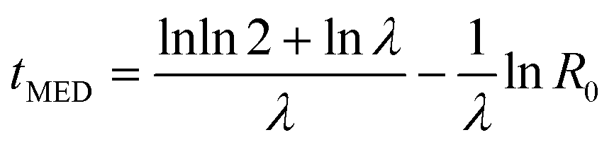
All the models make predictions for the scaling of the nucleation times with system size, and these predictions are different. So varying the size of the droplets, or the amount of material added to induce nucleation, are useful ways of testing the models. Also, as the system-size scaling is so variable, if we wish to use results from small droplets to make predictions for crystallisation in larger systems, then it is essential to have at least some understanding of the mechanism of nucleation.The characteristic timescale for nucleation can be measured using the median nucleation time tMED, which is by definition such that P(tMED) = 1/2. The simple model of a constant rate that is the same in all droplets, gives an exponential P(t) and tMED ~ 1/N for a nucleation rate k ∝ N the number of nucleation sites.
Earlier work by the author10 on the Weibull model of extreme-value statistics with β < 1, found that the median nucleation time varies with the number of nucleation sites as N−1/β. This means that the smaller the value of β the faster the nucleation timescale varies with N.
For the Pound–La Mer model in the k0 = 0 limit, tMED varies as
 | (14) |
The median nucleation time can also vary rapidly for this model. It diverges to infinity as m → ln2 ≃ 0.69 from above. This is because for m < ln2 more than half the droplets do not have any impurity particles in them and so never nucleate. In the other limit, that of large m, we can expand out the logarithm and tMED then scales as 1/m, i.e., one over the mean number of impurities. This is just we should expect as here the rate is in the thermodynamic limit.
The other model we considered was one where the nucleation rate was increasing with time. This gives a Gompertz distribution for P(t) which simplifies to a Gumbel function, eqn (11), in the limit R0 ≪ λ. Then the scaling of tMED is given by
 | (15) |
The median nucleation time scales logarithmically with the initial rate R0. We expect R0 ∝ N, the number of nucleation sites. Then we have a very slow, tMED ~ −lnN, scaling of the nucleation timescale with system size.
Having considered all three models, we can present an overview of the scalings of the median nucleation time
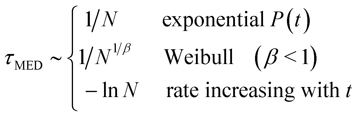 | (16) |
It is notable that for the systems with rates not in the thermodynamic limit (Weibull and Pound–La Mer), the median nucleation time varies rapidly with the number of nucleation sites. Here by rapidly we mean faster than 1/N. And by contrast when the nucleation time is set by the time for an initially slow rate (R0) to increase, the median nucleation time varies only slowly with N.
We end this section on scaling with size with a few example predictions. Diao et al.24 studied the crystallisation of ROY from solution. They did so with nothing added, and so where nucleation presumably occurs on impurities, and with the addition of poly(ethylene glycol) diacrylate (PEGDA) hydrogel particles. With the PEGDA hydrogel particles their fit to the surviving fraction of liquid drops yielded a best-fit value of β = 0.25. The prediction10 is then that on scaling the exposed surface area A of hydrogel, the median time to observe crystallisation will scale as A−4. Without the hydrogel particles, the best-fit value was found to be β = 0.37, and so at constant impurity concentration and assuming the impurities are in the bulk of the liquid drop bulk (not at the surface) the median nucleation time should scale with the volume V, as V−2.7. We should note that the data of Diao et al.24 are not perfectly fit by the stretched exponential function, and so there is probably considerable uncertainty in the exact value of the exponent, and the model itself is of course an approximation.
8. Large dynamic range in nucleation times
Carvalho and Dalnoki-Veress note that “upon cooling there is a population of droplets that nucleate at higher temperatures either because of heterogeneous nucleation or because the variations in the substrate result in a range of activation barriers to nucleation.” A fraction of their droplets crystallise while they are cooling to the temperature at which they will study isothermal crystallisation. As we can see in Fig. 4 most of the remainder crystallise over the 1500 s of their experiment. Clearly some of the droplets have barriers to nucleation that are so much lower than the barriers in the majority of the droplets that they cannot be studied in the same experiment. In effect the dynamic range of nucleation rates in the droplets is too large to be studied in an experiment that can only access timescales from seconds to a thousand seconds.This observation that the experiment is not able to study the nucleation times of all droplets is common.9,12,13,22–25,39,40,43 For example, in Pound and La Mer's work on tin droplets39 the P(t) curves often seem to be plateauing at fractions of tens of per cent, and in all cases some droplets remain unfrozen at the end of the experiment. Also, some droplets froze so rapidly that the nucleation times are at the time resolution of the experiments. Diao and coworkers observed similar behaviour.22,24
Experiments typically have a dynamic range of around 100 or more, so the fact that this is not enough to observe nucleation in all droplets implies that the dynamic range of nucleation rates is larger than this, possibly much larger. It appears that it is common that the rate is so far from the thermodynamic limit that the dynamic range of rates is at least a thousand and possibly much more.
9. Conclusions
“Everything should be made as simple as possible, but no simpler” is a very appealing principle, often attributed to Albert Einstein. The standard theory of nucleation is classical nucleation theory. This makes a number of simplifying assumptions.15,55,58 Essentially exact computer simulations of simple models shows that these simplifying assumptions are typically reasonable approximations.55,67,82 So for homogeneous nucleation, it seems likely that classical nucleation theory is reasonable for many systems.For example, in the important example of water, we used the Duft and Leisner8 data to obtain an estimated nucleation barrier of 55kT, at a supercooling of 36 °C. Computer simulations plus ideas from classical nucleation theory were used by Sanz et al.83 to estimate a barrier of 85kT. This was at a supercooling of 35 °C, and was for a simple water model (TIP4P/ice). Given that both numbers are estimates and the model for water is approximate, this is actually good agreement.
However, homogeneous nucleation is very much the exception. Heterogeneous nucleation is far more common. Here it is still possible that classical nucleation theory may provide a reasonable estimate of the barrier to nucleation at a particular point on a surface. But, apart from in the study of ice nucleation, it is often assumed that there is just one barrier and that this is the same in all droplets. The large volume of nucleation data in our class II, directly contradicts this assumption of a single barrier, as does the huge dynamic range of nucleation times often observed. So, this assumption is too simple. It should be abandoned, except where there is evidence for it, i.e., an exponential P(t).
To understand nucleation data, it would be very helpful to obtain direct information on the surfaces nucleation is actually occurring on. One way is to add material that induces nucleation. We then have a good idea of at least the basic chemistry of the surface. Also, Parmar et al.,59 Asanithi et al.28 and Jawor-Baczynska et al.79 have all done work on characterising objects in solution that affect nucleation. However the nucleation site may be only 10 nm across and so its geometry and any deviations from typical surface chemistry are unknown even in these cases. Future work should address this difficult problem of better characterising the sites where nucleation occurs. Finally, in many systems it may also be important to determine where in the liquid nucleation is occurring. For example, if it is occurring on an impurity, is this impurity at a surface or is it even at a contact line.15,18
Acknowledgements
It is a pleasure to acknowledge S. Akella, P. Asanithi, W. Cantrell, H. Christenson, S. Fraden, D. Frenkel, J. Keddie, L. Little, F. Meldrum, J. Mithen, B. Murray, A. Page, C.P. Royall, E. Sanz, R. Shaw, C. Valeriani, C. Vega and T. Whale for inspiring discussions, and to F. McKenzie for the invitation to write this review. I am grateful to K. Dalnoki-Veress, Y. Diao, R. Herbert, B. Kasemo, K.-K. Koo, J. Mithen, A. Myerson, B. Murray, T. Leisner, J.-B. Salmon, M. Schwind and B. Trout for permission to use their figures. I acknowledge financial support from EPSRC, under grant number EP/J006106/1, and for the support of PhD students.References
- J. Russo and H. Tanaka, Soft Matter, 2012, 8, 4206–4215 RSC.
- J. P. Mithen, private communication, 2013.
- H. R. Pruppacher and J. D. Klett, Microphysics of Clouds and Precipitation, Reidel Publishing, Dordrecht, 1978 Search PubMed.
- B. J. Murray, D. O'Sullivan, J. D. Atkinson and M. E. Webb, Chem. Soc. Rev., 2012, 41, 6519–6554 RSC.
- E. T. Lee, Statistical Methods for Survival Data Analysis, Wiley, 2nd edn, 1992 Search PubMed.
- D. R. Cox and D. Oakes, Analysis of Survival Data, Chapman and Hall, 1984 Search PubMed.
- R. P. Sear, Phys. Rev. E: Stat., Nonlinear, Soft Matter Phys., 2014, 89, 022405 CrossRef.
- D. Duft and T. Leisner, Atmos. Chem. Phys., 2004, 4, 1997 CrossRef CAS PubMed.
- J. L. Carvalho and K. Dalnoki-Veress, Phys. Rev. Lett., 2010, 105, 237801 CrossRef.
- R. P. Sear, Cryst. Growth Des., 2013, 13, 1329–1333 CAS.
- Y. Miyazawa and G. Pound, J. Cryst. Growth, 1974, 23, 45–57 CrossRef CAS.
- M. V. Massa and K. Dalnoki-Veress, Phys. Rev. Lett., 2004, 92, 255509 CrossRef.
- J. L. Carvalho and K. Dalnoki-Veress, Eur. Phys. J. E: Soft Matter Biol. Phys., 2011, 34, 6 CrossRef CAS PubMed.
- R. P. Sear, J. Phys.: Condens. Matter, 2007, 19, 466106 CrossRef.
- R. P. Sear, Int. Mater. Rev., 2012, 57, 328–356 CrossRef CAS PubMed.
- S. Suzuki, A. Nakajima, N. Yoshida, M. Sakai, A. Hashimoto, Y. Kameshima and K. Okada, Chem. Phys. Lett., 2007, 445, 37 CrossRef CAS PubMed.
- C. Gurganus, A. B. Kostinski and R. A. Shaw, J. Phys. Chem. Lett., 2011, 2, 1449 CrossRef CAS.
- C. Gurganus, A. B. Kostinski and R. A. Shaw, J. Phys. Chem. C, 2013, 117, 6195–6200 CAS.
- Y. Diao, M. E. Helgeson, Z. A. Siam, P. S. Doyle, A. S. Myerson, T. A. Hatton and B. L. Trout, Cryst. Growth Des., 2012, 12, 508–517 CAS.
- S. Jiang and J. H. ter Horst, Cryst. Growth Des., 2011, 11, 256 CAS.
- J. L. Quon, K. Chadwick, G. P. F. Wood, I. Sheu, B. K. Brettmann, A. S. Myerson and B. L. Trout, Langmuir, 2013, 29, 3292–3300 CrossRef CAS PubMed.
- Y. Diao, A. S. Myerson, T. A. Hatton and B. L. Trout, Langmuir, 2011, 27, 5324 CrossRef CAS PubMed.
- Y. Diao, M. E. Helgeson, A. S. Myerson, T. A. Hatton, P. S. Doyle and B. L. Trout, J. Am. Chem. Soc., 2011, 133, 3756 CrossRef CAS PubMed.
- Y. Diao, K. E. Whaley, M. E. Helgeson, M. A. Woldeyes, P. S. Doyle, A. S. Myerson, T. A. Hatton and B. L. Trout, J. Am. Chem. Soc., 2012, 134, 673–684 CrossRef CAS PubMed.
- R. J. Herbert, B. J. Murray, T. F. Whale, S. J. Dobbie and J. D. Atkinson, Atmos. Chem. Phys., 2014, 14, 1399–1442 Search PubMed.
- E. Saridakis and N. E. Chayen, Trends Biotechnol., 2009, 27, 99–106 CrossRef CAS PubMed.
- N. E. Chayen, E. Saridakis and R. P. Sear, Proc. Natl. Acad. Sci. U. S. A., 2006, 103, 597 CrossRef CAS PubMed.
- P. Asanithi, E. Saridakis, L. Govada, I. Jurewicz, E. W. Brunner, R. Ponnusamy, J. A. S. Cleaver, A. B. Dalton, N. E. Chayen and R. P. Sear, ACS Appl. Mater. Interfaces, 2009, 1, 1203 CAS.
- B. J. Murray, S. L. Broadley, T. W. Wilson, J. D. Atkinson and R. H. Wills, Atmos. Chem. Phys., 2011, 11, 4191 CrossRef CAS.
- J. D. Atkinson, B. J. Murray, M. T. Woodhouse, T. F. Whale, K. J. Baustian, K. S. Carslaw, S. Dobbie, D. O'Sullivan and T. L. Malkin, Nature, 2013, 498, 355358 CrossRef PubMed.
- D. Niedermeier, S. Hartmann, R. A. Shaw, D. Covert, T. F. Mentel, J. Schneider, L. Poulain, P. Reitz, C. Spindler, T. Clauss, A. Kiselev, E. Hallbauer, H. Wex, K. Mildenberger and F. Stratmann, Atmos. Chem. Phys., 2010, 10, 3601 CrossRef CAS.
- R. C. Sullivan, M. D. Petters, P. J. DeMott, S. M. Kreidenweis, H. Wex, D. Niedermeier, S. Hartmann, T. Clauss, F. Stratmann, P. Reitz, J. Schneider and B. Sierau, Atmos. Chem. Phys., 2010, 10, 11471–11487 CrossRef CAS.
- Y. Diao, T. Harada, A. S. Myerson, T. A. Hatton and B. L. Trout, Nat. Mater., 2011, 10, 867 CrossRef CAS PubMed.
- D. C. Johnston, Phys. Rev. B: Condens. Matter Mater. Phys., 2006, 74, 184430 CrossRef.
- F. Proschan, Technometrics, 1963, 375 CrossRef.
- P. Kabath, P. Stöckel, A. Lindinger and H. Baumgärtel, J. Mol. Liq., 2006, 125, 204 CrossRef CAS PubMed.
- A. Welti, F. Lüönd, Z. A. Kanji, O. Stetzer and U. Lohmann, Atmos. Chem. Phys., 2012, 12, 9893 CrossRef CAS.
- D. Knezic, J. Zaccaro and A. S. Myerson, J. Phys. Chem. B, 2004, 108, 10672–10677 CrossRef CAS.
- G. M. Pound and V. K. L. Mer, J. Am. Chem. Soc., 1952, 74, 2323–2332 CrossRef CAS.
- P. Laval, A. Crombez and J.-B. Salmon, Langmuir, 2009, 25, 1836–1841 CrossRef CAS PubMed.
- S. Teychené and B. Biscans, Cryst. Growth Des., 2011, 11, 4810–4818 Search PubMed.
- P. W. Wilson and A. D. J. Haymet, J. Phys. Chem. B, 2012, 116, 13472–13475 CrossRef CAS PubMed.
- M. Schwind, V. P. Zhdanov, I. Zoric and B. Kasemo, Nano Lett., 2010, 10, 931–936 CrossRef CAS PubMed.
- G. Vali, Atmos. Chem. Phys., 2008, 8, 5017 CrossRef CAS.
- P. J. Connolly, O. Möhler, H. Saathoff, R. Burgess, T. Choularton and M. Gallagher, Atmos. Chem. Phys., 2009, 9, 2805 CrossRef CAS.
- D. Niedermeier, R. A. Shaw, S. Hartmann, H. Wes, T. Clauss, J. Voigtländer and F. Stratmann, Atmos. Chem. Phys., 2011, 11, 8767 CrossRef CAS.
- S. L. Broadley, B. J. Murray, R. J. Herbert, J. D. Atkinson, S. Dobbie, T. L. Malkin, E. Condliffe and L. Neve, Atmos. Chem. Phys., 2012, 12, 287 CrossRef CAS.
- A. J. Durant and R. A. Shaw, Geophys. Res. Lett., 2005, 109, L20814 CrossRef.
- J.-W. Kim, J.-H. Park, H.-M. Shim and K.-K. Koo, Cryst. Growth Des., 2013, 13, 4688 CAS.
- I. Weidinger, J. Klein, P. Stckel, H. Baumgrtel and T. Leisner, J. Phys. Chem. B, 2003, 107, 3636–3643 CrossRef CAS.
- A. I. Toldy, A. Z. M. Badruddoza, L. Zheng, T. A. Hatton, R. Gunawan, R. Rajagopalan and S. A. Khan, Cryst. Growth Des., 2012, 12, 3977 CAS.
- L. Boinovich, A. Emelyanenko, V. V. Korolev and A. S. Pashinin, Langmuir, 2014, 30, 1659 CrossRef CAS PubMed.
- K.-K. Koo, private communication, 2013.
- E. B. Sirota and A. B. Herhold, Science, 1999, 283, 529 CrossRef CAS.
- R. P. Sear, J. Phys.: Condens. Matter, 2007, 19, 033101 CrossRef.
- A. J. Page and R. P. Sear, Phys. Rev. E: Stat., Nonlinear, Soft Matter Phys., 2009, 80, 031605 CrossRef CAS.
- Z. Dogic, Phys. Rev. Lett., 2003, 91, 165701 CrossRef.
- P. G. Debenedetti, Metastable Liquids, Princeton University Press, Princeton, 1996 Search PubMed.
- A. S. Parmar, P. E. Gottschall and M. Muschol, Biophys. Chem., 2007, 129, 224 CrossRef CAS PubMed.
- S. Akella and S. Fraden, to be published, 2014.
- A. J. Page and R. P. Sear, Phys. Rev. Lett., 2006, 97, 065701 CrossRef.
- A. J. Page and R. P. Sear, J. Am. Chem. Soc., 2009, 131, 17550 CrossRef CAS PubMed.
- L. O. Hedges and S. Whitelam, Soft Matter, 2012, 8, 8624 RSC.
- J. A. van Meel, R. P. Sear and D. Frenkel, Phys. Rev. Lett., 2010, 105, 205501 CrossRef.
- R. P. Sear, Phys. Rev. E: Stat., Nonlinear, Soft Matter Phys., 2004, 70, 021605 CrossRef.
- G. E. P. Box, Empirical Model-Building and Response Surfaces, Wiley, 1987 Search PubMed.
- S. Auer and D. Frenkel, Annu. Rev. Phys. Chem., 2004, 55, 333 CrossRef CAS PubMed.
- A. F. White and S. L. Brantley, Chem. Geol., 2003, 202, 479–506 CrossRef CAS PubMed.
- W. D. Callister, Materials Science and Engineering, John Wiley, 2010 Search PubMed.
- L. D. Mueller, T. J. Nusbaum and M. R. Rose, Exp. Gerontol., 1995, 30, 553 CrossRef CAS.
- E. Castillo, Extreme Value Theory in Engineering, Academic Press, San Diego, 1988 Search PubMed.
- E. Jondeau, S.-J. Poon and M. Rockinger, Financial Modeling Under Non-Gaussian Distributions, Springer, London, 2007 Search PubMed.
- J. Levine, Natl. Advis. Comm. Aeronaut., Tech. Notes, 1950, 2234 Search PubMed.
- R. P. Sear, Atmos. Chem. Phys., 2013, 13, 7215–7223 CrossRef CAS.
- M. Nicodemi, Extreme Value Statistics, in Encyclopedia of Complexity and System Science, ed. A. Robert, Meyers, Springer, 2009 Search PubMed.
- R. P. Sear, http://www.uniofsurreyblogs.org.uk/physics/2013/12/18/testing-models-learning-a-little-about-hot-tin/, 2013.
- D. Erdemir, A. Y. Lee and A. S. Myerson, Acc. Chem. Res., 2009, 42, 621–629 CrossRef CAS PubMed.
- A. F. Wallace, L. O. Hedges, A. Fernandez-Martinez, P. Raiteri, J. D. Gale, G. A. Waychunas, S. Whitelam, J. F. Banfield and J. J. De Yoreo, Science, 2013, 341, 885–889 CrossRef CAS PubMed.
- A. Jawor-Baczynska, J. Sefcik and B. D. Moore, Cryst. Growth Des., 2013, 13, 470–478 CAS.
- H. K. Christenson, CrystEngComm, 2013, 15, 2030–2039 RSC.
- P. G. Vekilov, Nanoscale, 2010, 2, 2346–2357 RSC.
- S. Auer and D. Frenkel, Nature, 2001, 409, 1020 CrossRef CAS PubMed.
- E. Sanz, C. Vega, J. R. Espinosa, R. Caballero-Bernal, J. L. F. Abascal and C. Valeriani, J. Am. Chem. Soc., 2013, 135, 15008–15017 CrossRef CAS PubMed.
| This journal is © The Royal Society of Chemistry 2014 |