 Open Access Article
Predicting power plant emissions using public data and machine learning†
Jiajun
Gu
,
Jeffrey A.
Sward
 and
K. Max
Zhang
 *
*
Sibley School of Mechanical and Aerospace Engineering, Cornell University, Ithaca, NY 14853, USA. E-mail: kz33@cornell.edu
First published on 18th October 2023
Abstract
Accurately predicting emissions from electric generating units using only publicly available information is an important but challenging task. It provides a critical link in evaluating the environmental impact of energy transitions in the power sector, makes it possible to engage stakeholders in electricity product cost modeling and electricity markets without accessing proprietary data, and serves as an auditing tool to detect anomalies in self-reported emissions data. However, the absence of proprietary data also limits the prediction accuracy. In this paper, we adopted two novel and effective strategies to overcome this challenge. First, we utilized not only the emission monitoring data (such as the Continuous Emission Monitoring System (CEMS) data) as previous studies did but also a variety of auxiliary datasets in the public domain such as the EPA Field Audit Checklist Tool (FACT). Second, we employed machine learning techniques (Extreme gradient boosting (XGBoost) and neural networks (NN)) to take advantage of the large amount of public data available. We evaluated the effectiveness of our strategies by predicting NOx, SO2, and CO2 emission rates for all thermal electric generating units in New York State (NYS). Two models were developed: a full model to take a full inventory of public information and a reduced model for use in data-limited scenarios based on unit-level features that could be derived from a simplified power systems economic dispatch model. The models performed well for NOx emission rates overall compared to the previous results, achieving R2 values over 0.9 for both the full and reduced models. XGBoost and NN were shown to outperform the Linear Regression (LR) model consistently and significantly, which was employed previously to estimate unit-level emissions, especially in reduced models with a limited number of features available. The predictions of SO2 and CO2 emission rates showed strong overall predictive performance as well. We recommend stricter enforcement of the data reporting procedure, providing emission control operational information, and obtaining related data from multiple sources in the public domain as key steps to further improve the emission predictions.
Environmental significancePredictive models of electric generating units' emissions are widely used in important energy and environmental applications. Models using only publicly available information have many societal benefits but often result in poor performance due to the lack of proprietary data. We tested two novel strategies, including (1) utilizing previously ignored but valuable public datasets on EGU operations to complement the emission data and (2) employing non-linear machine learning techniques compared to the traditional linear regression approach, to enhance the performance and showed that our models outperformed the previous ones consistently and significantly in predicting NOx, SO2, and CO2 emission rates. Therefore, we were able to present the most accurate open-accessible EGU emission prediction models for researchers, practitioners, and policymakers. |
1 Introduction
The power sector worldwide is currently in the midst of a rapid transition. For example, the fractions of the electricity generated in the U.S. from coal-fired and natural gas-fired power plants were 50% and 19% in 2015 as compared to 19% and 40% in 2020, respectively, according to the Energy Information Agency (EIA). Renewables dominated new electricity generation capacity added in 2020, consisting of wind (44%), solar (31%), and natural gas (22%). Since the power sector contributes substantially to emissions of greenhouse gases, criteria pollutants, and air toxics, these changes in the fuel mix improve air quality and mitigate climate change. The state-of-the-art method for assessing the air quality and health impacts of power system changes (such as high penetration of renewable energy) relies on linking a power systems unit commitment (UC) and economic dispatch (ED) model to a regional air quality model (e.g., CMAQ). One component crucial to this linkage is a prediction of electric generating unit (EGU) emissions (i.e., hourly, by pollutant type, for each EGU) given power dispatch profiles. In addition, a good emission prediction model is necessary for the economic environmental dispatch (EED) of generators, which minimizes both generation and environmental costs.Furthermore, as emission monitoring and control contributes to an increasing share of the EGU operational costs, the capacity to accurately predict EGU emissions can greatly improve electric production cost modeling, which is critical to ensuring efficient and reliable power system operations.1 Moreover, predicting EGU emissions using data in the public domain is particularly valuable because it makes broader stakeholder engagement possible by avoiding proprietary data internal to power system operators.
Nevertheless, predicting EGU emissions using public-only information accurately remains a challenging task. We have identified three main barriers to enhancing the EGU prediction accuracy, described as follows.
First, there are no effective tools to take advantage of the large number of datasets available in the public domain. For example, EGUs in the U.S. with a nameplate capacity over 25 MW equivalent (or combusting fuels with a sulfur content greater than 0.05% by mass) are required by law to be equipped with continuous emissions monitoring systems (CEMS). All data records collected by CEMS since 1990 are publicly available. However, our literature survey revealed that most of existing studies on predicting EGU emissions focused on a single unit using various data-driven techniques including autoregression,2,3 neural networks,4–9 SVM,10,11 and ELM.12 A commonality among these studies is access to detailed EGU operational data that exists outside of the public domain, which makes repeating or generalizing such approaches to other units infeasible. By contrast, only linear regression (LR) has been reported for modeling CEMS data from a large EGU fleet.
Second, previous efforts in EGU emission prediction have not taken advantage of all the relevant public datasets available besides the emission monitoring data such as CEMS. For example, while intended to facilitate field audits of facilities that report CEMS data, the USEPA Field Audit Checklist Tool (FACT) allows users to view not only CEMS data but also monitoring plans and quality assurance plans. Users can obtain the corresponding method of determination codes (MODC) for CEMS data to differentiate data points based on measurement from those based on calculations. Therefore, MODC provides further insight in interpreting CEMS data.
Third, predicting NOx emissions, which are a direct public health concern in the form of NO2, a criteria pollutant as well as a primary ozone precursor, presents additional challenge as emission control technologies, both combustion-based and post-combustion, affect NOx emissions differently, and their effectiveness depends on EGU operating conditions as NOx formation during combustion depends on complex chemical kinetics occurring within turbulent flows.13,14 Therefore, the need for improving the prediction of NOx emissions is imperative.
In this paper, we addressed the barriers described above by developing machine learning (ML)-based models to predict NOx, SO2, and CO2 emission rates and utilizing a variety of public datasets in addition to CEMS data. We thoroughly evaluated the effectiveness of this approach by predicting emissions from all thermal EGUs larger than 25 MW in New York State (NYS) on a year-by-year and unit-by-unit basis with increasing prediction horizons and interpreted the modeling results utilizing permutation importance. NYS was chosen as the focal area in our study as the EGU fleet in NYS is large and diverse. The 328 thermal EGUs, span six generation types and eight fuel types providing opportunities for detailed unit-by-unit analyses. Furthermore, the power system in NYS became coal-free in 2020, foreshadowing the future generation mix across the U.S. We aimed to make these models transparent by using only publicly available data and generalizable among different units.
The paper is organized as follows. We first introduce the data collection (Section 2.1) and data cleaning process (Section 2.2), followed by a description of model implementation (Section 2.3). Then we describe the model evaluation procedure (Section 2.4) and the approaches used to analyze and interpret the models (Section 2.5). Finally, we show the model's predictive performance and analysis results (Section 3).
2 Methods
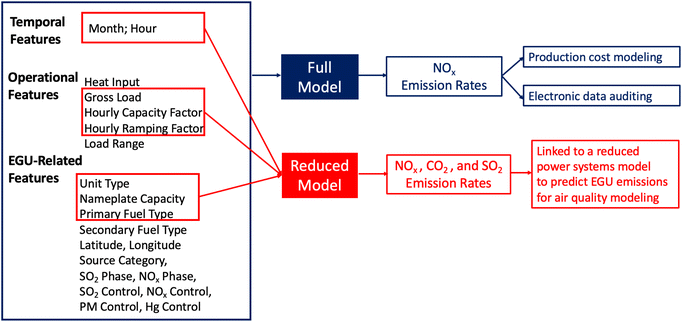
Fig. 1 shows the key steps of our study. The rest of Section 2 is structured to elaborate each of the key steps. | ||
| Fig. 1 Key steps in applying machine learning techniques to predict EGU emissions using public datasets. | ||
2.1 Data collection
We downloaded hourly, unit-level CEMS data for New York State (NYS) from 2015 to 2019 using the Air Markets Program Data (AMPD) tool15 from USEPA. Among the variables in the raw CEMS data, we aimed to predict hourly emission rates of NOx, SO2, and CO2. But these must be derived in different ways. The NOx concentrations in ppm and diluent concentration in % O2 or CO2 are measured in a NOx-diluent monitoring system,16 and then the hourly NOx emission rate in pounds per mmBtu is calculated.17 The NOx emission rate in pounds per hour is further calculated by multiplying the hourly NOx emission rate in pounds per mmBtu by the reported hourly heat input in mmBtu per hour and the operating time.17 The SO2 emission rate in pounds per hour was estimated using the default SO2 emission rate in pounds per mmBtu and the reported heat input rate in mmBtu per hour for most of the gas-fired units.18 For the oil-fired units (and some of the gas-fired units), the SO2 emission rate was calculated using the reported fuel consumption rate and the measured sulfur content.18 The CO2 emission rate in tons per hour was estimated using the recorded heat input rate in mmBtu per hour or quantified by a CO2 monitoring system together with a flow monitoring system.19 In the following discussion, we refer to these target variables as “CAMD-derived emission rates”.After removing non-contributing variables (i.e., those with constant or many missing values), we selected 16 features from the CEMS data for the predictive models, including month, hour, gross load, heat input, source category, SO2 phase, NOx phase, unit type, primary fuel type, secondary fuel type, SO2 control, NOx control, PM control, Hg control, facility latitude, and facility longitude. We added 4 additional features, which characterize EGU operational conditions, including the nameplate capacity, load range, hourly capacity factor, and hourly ramping factor. The nameplate capacity for each EGU and the hourly load range were collected using the USEPA Field Audit Checklist Tool (FACT). The hourly capacity factor and hourly ramping factor at hour t were calculated as follows:
 | (1) |
 | (2) |
The hourly load range, capacity factor, and ramping factor aim to train the models that higher emissions are likely to occur during part-load operation and ramping, respectively. In total, this resulted in 20 features. We then converted all the categorical features into numeric values using one-hot encoding, which converts one categorical value into a group of digits with a single “1” (hot) and all others “0” representing the same categorical value.
2.2 Data cleaning
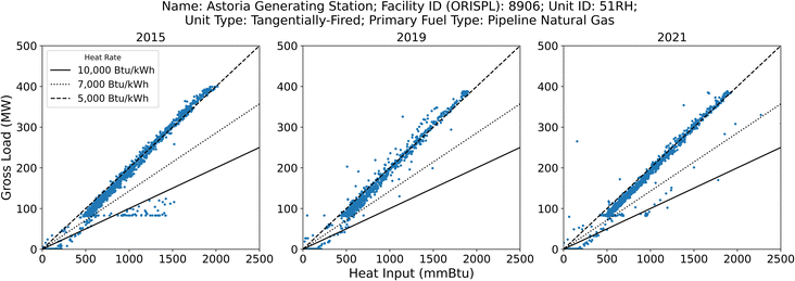
For the NOx emissions and heat input, we checked the corresponding method of determination codes (MODC) available using the USEPA FACT and removed substitute data points that were fully calculated instead of measurement-based. We deleted data points with no operating time or gross load as no emissions were generated during those conditions. We removed data points with partial operating hours to eliminate startup and shutdown conditions. Emissions associated with startup and shutdown conditions will be investigated in a future study.In addition, we screened the heat rate (inverse of the thermal efficiency) data to identify anomalies. We identified three different heat rate regimes: ∼5000 Btu kW−1 h−1, ∼7000 Btu kW−1 h−1, and ∼10![[thin space (1/6-em)]](https://www.rsc.org/images/entities/char_2009.gif) 000 Btu kW−1 h−1. Note that 5000 Btu kW−1 h−1, or ∼70% thermal efficiency, is physically impossible for thermal EGUs and may indicate reporting errors. For example, Fig. 2 depicts hourly recorded heat input versus gross load in 2015, 2019, and 2021, respectively, for Unit 51RH at the Astoria Generating Station (Facility ID: 8906). It is a tangentially-fired unit with pipeline natural gas (PNG) as the primary fuel type. A majority of the data points fall into the ∼5000 Btu kW−1 h−1 heat rate regime, which was also reported in a 2018 study.20 We conducted further investigation into this facility by examining its Title V permit from the New York Department of Environmental Conservation (NYSDEC). We gather that this unit is a twin-furnace boiler that exhausts emissions through two stacks, counted as two units (Unit 51RH and Unit 52SH). Therefore, we attribute these nonphysical heat rates to a systematic reporting error – or loophole. Specifically, dividing the gross load for the full boiler by the heat input for each individual furnace would halve the true heat rate, which could be the case here given the consistent trends shown in Fig. 2. In the current study, we removed data points with unrealistic heat rates (<6000 Btu kW−1 h−1). For future study, we recommend stricter enforcement of data report procedures by USEPA to eliminate those reporting errors.
000 Btu kW−1 h−1. Note that 5000 Btu kW−1 h−1, or ∼70% thermal efficiency, is physically impossible for thermal EGUs and may indicate reporting errors. For example, Fig. 2 depicts hourly recorded heat input versus gross load in 2015, 2019, and 2021, respectively, for Unit 51RH at the Astoria Generating Station (Facility ID: 8906). It is a tangentially-fired unit with pipeline natural gas (PNG) as the primary fuel type. A majority of the data points fall into the ∼5000 Btu kW−1 h−1 heat rate regime, which was also reported in a 2018 study.20 We conducted further investigation into this facility by examining its Title V permit from the New York Department of Environmental Conservation (NYSDEC). We gather that this unit is a twin-furnace boiler that exhausts emissions through two stacks, counted as two units (Unit 51RH and Unit 52SH). Therefore, we attribute these nonphysical heat rates to a systematic reporting error – or loophole. Specifically, dividing the gross load for the full boiler by the heat input for each individual furnace would halve the true heat rate, which could be the case here given the consistent trends shown in Fig. 2. In the current study, we removed data points with unrealistic heat rates (<6000 Btu kW−1 h−1). For future study, we recommend stricter enforcement of data report procedures by USEPA to eliminate those reporting errors.
Finally, 253![[thin space (1/6-em)]](https://www.rsc.org/images/entities/char_2009.gif) 479–329
479–329![[thin space (1/6-em)]](https://www.rsc.org/images/entities/char_2009.gif) 202 effective data points remained for modeling depending on the year representing 113 units from four different unit types: combined cycle, combustion turbine, tangentially-fired, and dry bottom wall-fired boiler. Table 1 summarizes the 2018 statistics of NOx emission rates for different unit types. Note that while the values in the table differ by year the order of magnitudes remain consistent.
202 effective data points remained for modeling depending on the year representing 113 units from four different unit types: combined cycle, combustion turbine, tangentially-fired, and dry bottom wall-fired boiler. Table 1 summarizes the 2018 statistics of NOx emission rates for different unit types. Note that while the values in the table differ by year the order of magnitudes remain consistent.
| Unit type | Number of units | Number of data points | Mean | Standard deviation | Percentile | ||||
|---|---|---|---|---|---|---|---|---|---|
| 25th | 50th | 75th | 99th | 100th | |||||
| Combined cycle | 56 | 214![[thin space (1/6-em)]](https://www.rsc.org/images/entities/char_2009.gif) 580 580 |
19.8 | 20.3 | 7.7 | 12.5 | 23.9 | 89.1 | 621.8 |
| Combustion turbine | 29 | 30![[thin space (1/6-em)]](https://www.rsc.org/images/entities/char_2009.gif) 099 099 |
13.0 | 19.2 | 3.6 | 4.1 | 26.1 | 43.9 | 302.0 |
| Tangentially-fired | 21 | 46![[thin space (1/6-em)]](https://www.rsc.org/images/entities/char_2009.gif) 895 895 |
129.3 | 188.1 | 33.2 | 81.5 | 151.6 | 1116.5 | 2153.7 |
| Dry bottom wall-fired boiler | 6 | 3125 | 139.0 | 274.0 | 18.1 | 21.8 | 75.1 | 1296.3 | 2350.6 |
2.3 Model implementation
We created two distinct ML-based models: a full model and a reduced model as illustrated in Fig. 3. The full model utilizes all the information contained in the public databases and is designed to be incorporated into a production cost model and/or serve as an electronic auditing tool to detect anomalies in the self-reported continuous emissions monitoring system (CEMS) data. This full model has the potential to facilitate power systems planning, identify regulatory compliance issues, improve data quality, and reduce emissions. The reduced model is designed to be linked to a power systems model to predict EGU emissions for air quality modeling. Since power systems models often rely on simplified network topologies, the reduced model only uses features that can be readily obtained from such power systems models.Using linear regression (LR) as a benchmark, we screened several ML algorithms, including support vector machine (SVM), decision tree, adaptive boosting (AdaBoost), random forest (RF), extreme gradient boosting (XGBoost), and neural networks (NN), by comparing their full model performance. Among these algorithms, XGBoost and NN consistently outperformed the others. Therefore, we focused on XGBoost and NN for detailed analysis. All the models were implemented using the scikit-learn library in Python.21 A brief description of XGBoost and NN is as follows.
XGBoost expands upon the principle of traditional gradient boosting algorithms, which iteratively combines weak learners (e.g. shallow decision trees) into a strong learner to reduce the model bias and improve overall accuracy. It adds both L1 and L2 regulation to prevent model overfitting, and with the parallelization of individual tree building, offers improved computational efficiency as well.
The NN implemented in this study is a dense sequential (feed forward) neural network, which comprises two densely connected hidden layers, and an output layer that returns a single, continuous value. It is a multilayered perception model utilizing the back-propagation technique for training. The multiple layers and non-linear activation functions enable it to distinguish data that is not linearly separable.
Considering that the heat input rate plays a key role in calculating the SO2 and CO2 emission rates and is typically not available in the reduced-form representations of the power system for a future scenario, we built reduced models to estimate the hourly heat input. Then we calculated the SO2 and CO2 emission rates using the equations specified in Appendix D to Part 75 of 40 CFR18 (for the SO2 emission rate) and Appendix G to Part 75 of 40 CFR19 (for the CO2 emission rate):
| SO2 emission rate (pounds per hour) = 0.0006 pounds per mmBtu × hourly heat input (mmBtu per hour) | (3) |
 | (4) |
2.4 Model evaluation
We split the data into training and test sets in three different ways, which are depicted in Fig. 4. First, in order to test the forecasting ability of the model considering interannual variability, we implemented the models by training on the previous year's data and testing on the following year's data, year-by-year from 2015 to 2019. Second, in order to investigate how far ahead the model is capable of making predictions, we evaluated the model with different prediction horizons. Using the data from 2019 as the test set, we trained the model with the data from 2015 to 2018 (1 year prediction horizon), from 2015 to 2017 (2 year prediction horizon), from 2015 and 2016 (3 year prediction horizon), and with the data from 2015 (4 year prediction horizon). Note that the prediction horizon increases from 1 to 4 years. Third, in order to find the amount of training data needed to achieve optimal performance, we drew learning curves of model performance by training models with different amounts of data from a half-year to four years. Data were combined from the odd-numbered months (January, March, May, July, September, and November) to create the half-year.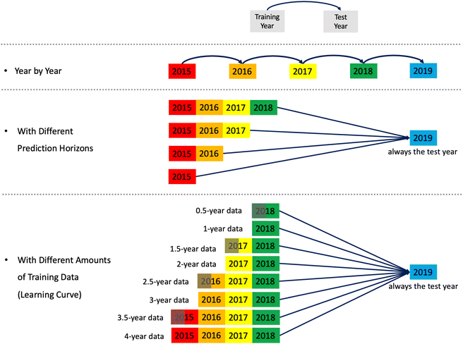 | ||
| Fig. 4 Sketch of the model evaluation in tree different ways: year by year, with different prediction horizons, and with different amounts of training data (learning curve). | ||
To evaluate the models' performance, we employed the coefficient of determination (R2), root mean square error (RMSE), and normalized RMSE (nRMSE) as the main metrics. R2 measures the proportion of the variance that is explained by the model indicating how well the model replicates the data. RMSE measures the square root of the average squared difference between the predictions and observations. We normalized RMSE by the standard deviation, referred to as nRMSE, to take into account the slightly different scales of data points in different years.
2.5 Model interpretation
We conducted two independent analyses to characterize the models' predictive performance in terms of identifying key features and making meaningful representations from the data. First, we examined the model performance at the unit level. Second, we measured model feature importance using permutation importance23 for all features in the full model. Briefly, this method randomly shuffles a feature's value and determines the feature's importance based on the respective performance decrease. It is model-agnostic but note that the permutation importance can be misleading when features are highly correlated, resulting in lower importance values. Therefore, we only kept one feature among a group of correlated features (Pearson correlation coefficient >0.8) when calculating permutation importance and assigned the same permutation importance to all the correlated features within the group.3 Results and discussion
3.1 Overall model predictive performance on NOx emission rates
Table 2 summarizes the overall predictive performance of NOx emission rates for the full and reduced models, respectively, using the year-by-year evaluation approach. Both XGBoost and NN show strong overall predictive performance in terms of R2, RMSE (pounds per hour), and nRMSE and outperform LR. In the full model (Table 2), the R2 for LR is between 0.82 and 0.91 with nRMSE ranging from 0.011–0.012, while the R2 for XGBoost and NN R2 can achieve 0.95–0.96 with nRMSE ranging from 0.005–0.008. XGBoost and NN models perform similarly, with the difference in R2 less than 0.01, in RMSE less than 1.4 pounds, and in nRMSE of less than 0.001. Both XGBoost and NN perform consistently in terms of R2 and nRMSE for different training and test years with a one-year prediction horizon.| Training year | Test year | Full model | ||||||||
|---|---|---|---|---|---|---|---|---|---|---|
| LR | XGBoost | NN | ||||||||
| R 2 | RMSE | nRMSE | R 2 | RMSE | nRMSE | R 2 | RMSE | nRMSE | ||
| 2015 | 2016 | 0.91 | 26.2 | 0.011 | 0.96 | 17.7 | 0.007 | 0.96 | 18.5 | 0.008 |
| 2016 | 2017 | 0.89 | 26.3 | 0.012 | 0.96 | 16.0 | 0.007 | 0.96 | 16.3 | 0.007 |
| 2017 | 2018 | 0.90 | 29.4 | 0.012 | 0.95 | 21.0 | 0.009 | 0.95 | 19.6 | 0.008 |
| 2018 | 2019 | 0.82 | 23.9 | 0.011 | 0.96 | 11.0 | 0.005 | 0.96 | 11.8 | 0.005 |
As shown in Table 3, XGBoost and NN for the reduced model, which contains far fewer features than the full model, still perform well with R2 between 0.86–0.93 and nRMSE between 0.007–0.015. By contrast, LR performs poorly, with much lower R2 between 0.29–0.54 and much higher nRMSE between 0.021–0.031. The reduced XGBoost models perform slightly better than the reduced NN models (i.e., slightly higher R2; slightly lower RMSE and nRMSE), with a difference in R2 of less than 0.03, RMSE of less than 4.5 pounds, and nRMSE of less than 0.001. The reduced model is somewhat more sensitive to the chosen training and test years compared with the full model.
| Training year | Test year | Reduced model | ||||||||
|---|---|---|---|---|---|---|---|---|---|---|
| LR | XGBoost | NN | ||||||||
| R 2 | RMSE | nRMSE | R 2 | RMSE | nRMSE | R 2 | RMSE | nRMSE | ||
| 2015 | 2016 | 0.54 | 59.7 | 0.025 | 0.93 | 22.9 | 0.010 | 0.90 | 27.4 | 0.011 |
| 2016 | 2017 | 0.39 | 62.9 | 0.028 | 0.93 | 21.8 | 0.010 | 0.90 | 25.2 | 0.011 |
| 2017 | 2018 | 0.38 | 72.7 | 0.031 | 0.86 | 34.2 | 0.015 | 0.86 | 34.2 | 0.015 |
| 2018 | 2019 | 0.29 | 47.5 | 0.021 | 0.91 | 16.4 | 0.007 | 0.90 | 17.8 | 0.008 |
To summarize, compared with applying linear models, applying non-linear algorithms to predict the EGU NOx emission rate can significantly enhance model performance and achieve much higher prediction accuracy, especially for models with fewer features.
3.2 Unit-level model predictive performance on NOx emission rates
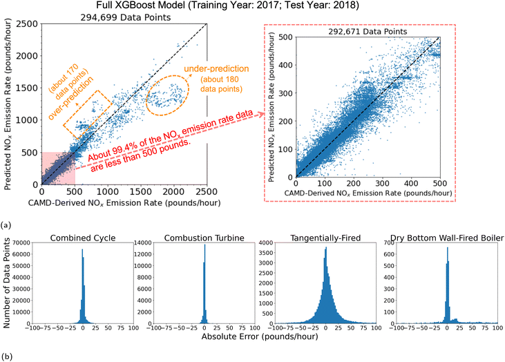
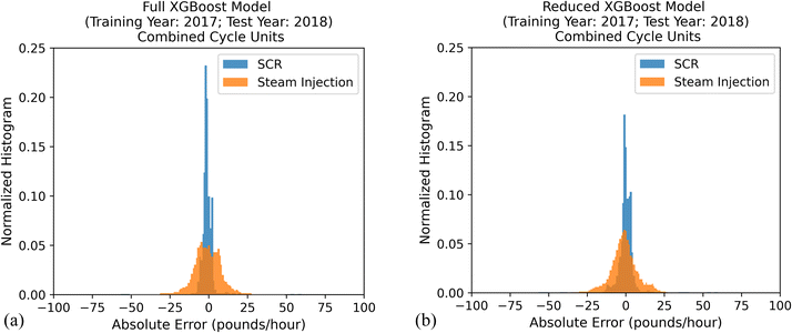
We use the full XGBoost model trained on 2017 data and tested on 2018 data as an example to investigate the details of model performance. Fig. 5a presents the scatter plots of CAMD-derived vs. predicted NOx emission rates on different scales (2500 pounds per hour in the left plot and 500 pounds per hour in the right plot). About 99.4% of the NOx emission rates fell below 500 pounds in 2018, i.e., within the region shown in the right scatter plot. The overall trend follows the identity line indicating good overall model predictive performance (R2 = 0.95, nRMSE = 0.009). Fig. 5b illustrates the corresponding distributions of the absolute errors, i.e., the difference between the predicted NOx emission rates and the CAMD-derived NOx emission rates, grouped by different unit types including combined cycle, combustion turbine, tangentially-fired, and dry bottom wall-fired boiler. The absolute errors are concentrated around 0 for all unit types. But the tangentially-fired units have the widest error distribution as a result of much larger NOx emission rates than the other types of units. As shown in Table 1, the NOx emission rates from the tangentially-fired units averaged 120.0 pounds per hour, and some extreme values exceeded 2000 pounds per hour in 2018.The models also captured the impact of emission control technologies. Fig. 6 compares the distributions of absolute prediction errors for combined cycle units equipped with selective catalytic reduction (SCR) and those with steam injection, using the full model (Fig. 6a) and the reduced model (Fig. 6b), respectively. Note that the steam injection units typically have much higher NOx emission rates than the SCR units, as SCR is more effective in reducing NOx emissions than steam injection. All the distributions are centered around a zero mean, indicating that the models generally captured emission rate magnitude differences. Higher emission rates and more dynamic combustion conditions in the steam injection units led to higher prediction errors for these units than the SCR units.
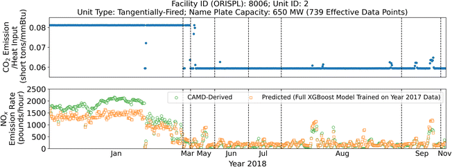 | ||
| Fig. 7 The ratios between CO2 emissions and heat input (upper), and CAMD-derived versus predicted NOx emission rates (bottom, R2 = 0.86) from Unit 2 of the Roseton Generating LLC facility in Newburgh, NY (Facility ID: 8006) in 2018, with abnormal high NOx emission rates in January corresponded with the under-prediction zone shown in the left scatter plot in Fig. 5a. | ||
Another over-prediction zone highlighted by the orange dashed box in the left scatter plot in Fig. 5a, contains about 170 data points. Most of these come from one of the tangentially-fired units within the Ravenswood Generating Station in Long Island City, NY (Facility ID: 2500; Unit ID: 30). As shown in the bottom plot of Fig. 8, these mispredictions occurred in June, July, August, and September 2018 with NOx emission rates (bottom plot) at relatively high levels. Although the unit uses residual oil as the primary fuel and PNG as the secondary fuel, the ratios between CO2 emissions and heat input suggest that the unit was burning PNG most of the time in 2018 as shown in the upper plot of Fig. 8. When those mispredictions occurred, the ratios exceeded 0.059 (but remained below 0.081) indicating the supplement of residual oil, which results in the over-predictions of these emission rates. During the remainder of the year, the model performed well with predicted rates following calculated rates closely resulting in a unit-level R2 of 0.88.
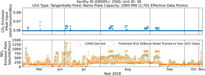 | ||
| Fig. 8 The ratios between CO2 emissions and heat input (upper), and CAMD-derived versus predicted NOx emission rates (bottom, R2 = 0.88) from Unit 30 of the Ravenswood Generating Station facility in Long Island City, NY (Facility ID: 2500) in 2018, with NOx emission rates of about 160 data points over-predicted in June, July, August and September corresponded with the over-prediction zone shown in the left scatter plot in Fig. 5a. | ||
In summary, for the tangentially-fired units with high NOx emission rates, the model captures the correct temporal trend but mispredicts the magnitude of the emission rate when an EGU operates abnormally (e.g., switches fuel or is co-fired with different fuels). Furthermore, it is very important to include both CO2 and heat input as features to predict NOx emissions.
3.3 Features' importance in predicting NOx emission rates
We quantified feature importance for the full model using permutation importance. Permutation importance measures the decrease in model performance when randomly shuffling a feature's value. Using the full model for the NOx emission rate trained on 2017 data and tested on 2018 data as examples, Fig. S1a in the ESI† ranked the feature importance for the full XGBoost model, and Fig. S1b† for the full NN model. The bars (corresponding to the left axis) represent the permutation importance of the top 20 features with each feature ranked from most to least important, and the blue dots and green triangles (corresponding to the right axis) show the model performance in terms of R2 for training data and test data, respectively.Heat input, gross load, and CO2 emission rates are the most influential features. With these three features, the test R2 reaches 0.90 for the full XGBoost model and 0.86 for the full NN model. Notice that these three features are highly correlated, so when calculating the permutation importance, they were combined to form one group and assigned the same permutation importance.
For the full NN model, nameplate capacity and SO2 emission rate rank fourth and fifth with relatively larger permutation importance values (>0.1) than the remaining features. For the full XGBoost model, SO2 emission rate, tangentially-fired unit type, hourly capacity factor, and load range rank fourth – seventh with permutation importance values larger than 0.1. Historically, tangentially fired boilers were widely used in coal-fired power plants but were converted to burn natural gas as the primary fuel type in NYS. As mentioned in Section 3.2, the NOx emissions from the tangentially-fired boilers were overall much higher than the other types of units. Therefore, the model is able to differentiate those units from the other types, and the corresponding features indicating this specific unit type show relatively high permutation importance.
3.4 Varying prediction horizon and learning curve for NOx emission rates
Fig. S2a in the ESI† shows the model performance on 2019 data with prediction horizons increasing from 1 to 4 years. Overall, the model performance only deteriorates slightly when the prediction horizon increases. For example, with a 4 year prediction horizon, i.e., when the model was trained only using data from 2015, the model still achieves an acceptable range with R2 ranging from 0.88 to 0.92 depending on the model type.Fig. S2b in the ESI† depicts the model performance in terms of R2 with respect to the amount of data used, starting with a half-year of data from 2018, and finishing with 4 years of data from 2015 to 2018. In all cases, the test data came from 2019. There is an increasing trend in R2, though small, for each addition of data to the training set. With a half-year of data from 2018, both the full and reduced models already achieve satisfactory performance, i.e., a full model R2 larger than 0.93 and a reduced model R2 larger than 0.87. For the XGBoost model, R2 for the full model increases from 0.95 (trained with a half-year of data from 2018) to 0.96 when another half-year of data is added. It then remains at 0.96 even with all four years of data added. R2 for the reduced XGBoost model increases from 0.87 to 0.90 going from a half-year to a full year of data and finally reaches 0.91 as more data are added. For the NN model, R2 for the full model increases from 0.93 (trained with a half-year of data from 2018) to 0.94 with the full year of data added, and finally reaches 0.96 with all four years of data. R2 for the reduced NN model increases from 0.87 (trained with a half-year of data from 2018) to 0.91 with all four years of data. A deviation from the increasing trend in model performance occurs for the NN models when the 2016 data are added.
3.5 Reproducing SO2 and CO2 emission rates with predicted hourly heat input
As denoted in eqn (3) and (4), the SO2 and CO2 emission rates are derived based on heat input. Therefore, in order to reproduce the SO2 and CO2 emission rates for the reduced model, we implemented an additional reduced model to predict the hourly heat input. The model was trained on the previous year's data and tested on the current year's data, year by year from 2015 to 2019. Both XGBoost and NN models show strong overall predictive performance in terms of R2 (0.98–0.99). Fig. 9a shows a scatter plot of the measured vs. predicted hourly heat input from the reduced XGBoost model for heat input trained on 2017 data and tested on 2018 data as an example. | ||
| Fig. 9 The scatter plot of (a) measured versus predicted hourly heat input from the reduced XGBoost model (trained on 2017 data and tested on 2018 data); (b) CAMD-derived versus predicted SO2 emission rates for gas-fired hours only, with the predicted values calculated by eqn (3) using the predicted hourly heat input; (c) CAMD-derived versus predicted CO2 emission rates, with the predicted values calculated by eqn (4) using the predicted hourly heat input. | ||
We then calculated the SO2 emission rates (for gas-fired hours only) and CO2 emission rates using eqn (3) and (4), respectively, and the predicted hourly heat input. Fig. 9b and c show CAMD-derived vs. predicted SO2 and CO2 emission rates, respectively, for 2018. The models for SO2 and CO2 both perform well, which strongly depend on the predicted hourly heat input.
4 Conclusions
Predictive models of emissions from electric generating units are used in a wide range of important energy and environmental applications. Driven by a need for improved emissions predictions, we developed machine learning-based models to predict the emission rates of several pollutants using a variety of publicly available datasets. The models achieved an unprecedented high level of performance. For example, the R2 value for NOx emission rates reached as high as 0.96 and 0.93 for both the full and reduced models, respectively. These models also show the capability of differentiating NOx control technologies. In order to reproduce calculation-based SO2 and CO2 emission rates, we built a reduced model to estimate the heat input, which plays a key role in calculating the SO2 and CO2 emission rates. Both XGBoost and NN models show strong overall predictive performance with R2 reaching 0.95–0.99. Those results demonstrated that our proposed strategies, i.e., applying machine learning techniques and using diverse datasets, have been effective. To the best of our knowledge, we were able to present in this paper the most accurate open-accessible unit-level emission prediction models for researchers, practitioners, and policymakers.There are a number of future steps to further enhance our capability in predicting unit-level emissions. First, we identified and removed the data points with unrealistic heat rates (Section 2.2). Resolving the corresponding data issue by strictly enforcing the reporting protocols is important for improving the data quality. Second, we excluded the data points associated with the generator startup and shutdown in this study. Such conditions only accounted for about 5% of the entire dataset. However, startup or shutdown can lead to exceedingly high emission rates (and only last for a short period of time), making them worthy of a dedicated study. Third, the methodology presented in this paper can be readily applied to other regions. Our study focused on the generation fleet in New York State. This focused approach enabled us to conduct detailed unit-by-unit analyses and seek advice from state experts. Our overall approach can be readily implemented for modeling power plant emissions in other regions in the U.S., and it is generally applicable to other countries where public datasets of power plant emissions are available. Expanding the work to other regions will create a larger dataset, which should further improve the accuracy of the models. Finally, we found that the USEPA Field Audit Checklist Tool (FACT) provides valuable information, including additional generator characteristics, operating conditions, and methods of data determination, that are not available from the Air Markets Program Data (AMPD) tool. Follow-up studies that fully take advantage of the information presented in FACT, or any other informative features available from the public domain (e.g., the generator model year), can provide additional insight into predicting unit-level emissions.
Conflicts of interest
There are no conflicts to declare.Acknowledgements
The authors would like to acknowledge the support from the New York State Energy Research and Development Authority (NYSERDA) and the kind assistance by Charles Frushour, Michael Heese and Justine Huetteman at the U.S. Environmental Protection Agency (USEPA) through the EmPOWER Air Data Challenge. The authors appreciate the valuable discussions with Ben Cohen at the New York Independent System Operator (NYISO), Ona Papageorgiou and Michael Sheehan at New York State Department of Environmental Conservation (NYSDEC) as well the generous contributions from Huilin Zhang, Ye Jiang, Yingying Yu, Zimo Zheng and Akash Kumar at Cornell University. JAS’ work was supported by the National Science Foundation Graduate Research Fellowship under grant number DGE-1650441.References
- E. Kahn, Oper. Res., 1995, 43, 388–398 CrossRef.
- Y. Tunckaya and E. Koklukaya, J. Energy Inst., 2015, 88, 118–125 CrossRef CAS.
- S. M. Safdarnejad, J. F. Tuttle and K. M. Powell, Comput. Chem. Eng., 2019, 124, 62–79 CrossRef CAS.
- J. Song, C. E. Romero, Z. Yao and B. He, Knowl Based Syst., 2016, 118, 4–14 CrossRef.
- F. Wang, S. Ma, H. Wang, Y. Li and J. Zhang, Control Eng. Pract., 2018, 80, 26–35 CrossRef.
- P. Tan, B. He, C. Zhang, D. Rao, S. Li, Q. Fang and G. Chen, Energy, 2019, 176, 429–436 CrossRef CAS.
- D. Adams, D.-H. Oh, D.-W. Kim, C.-H. Lee and M. Oh, J. Cleaner Prod., 2020, 270, 122310 CrossRef CAS.
- X. Hu, P. Niu, J. Wang and X. Zhang, Atmos. Pollut. Res., 2020, 11, 1084–1090 CrossRef CAS.
- G. Yang, Y. Wang and X. Li, Energy, 2020, 192, 116597 CrossRef CAS.
- Y. Lv, J. Liu, T. Yang and D. Zeng, Energy, 2013, 55, 319–329 CrossRef CAS.
- J. F. Tuttle, L. D. Blackburn and K. M. Powell, Comput. Chem. Eng., 2020, 141, 106990 CrossRef CAS.
- P. Tan, J. Xia, C. Zhang, Q. Fang and G. Chen, Energy, 2016, 94, 672–679 CrossRef CAS.
- S. Hill and L. D. Smoot, Prog. Energy Combust. Sci., 2000, 26, 417–458 CrossRef CAS.
- P. Glarborg, J. A. Miller, B. Ruscic and S. J. Klippenstein, Prog. Energy Combust. Sci., 2018, 67, 31–68 CrossRef.
- United States Environmental Protection Agency (EPA), Washington, DC: Office of Atmospheric Programs, Clean Air Markets Division, available from EPA’s Air Markets Program Data web site: https://ampd.epa.gov, accessed Aug, 2020 Search PubMed.
- Office of the Federal Register National Archives and Records Administration, 40 CFR Part 75.10 – General operating requirements, available from: https://www.law.cornell.edu/cfr/text/40/75.10, accessed Aug, 2020 Search PubMed.
- Office of the Federal Register National Archives and Records Administration, 40 CFR Subpart H – NOX Mass Emissions Provisions, available from: https://www.law.cornell.edu/cfr/text/40/part-75/subpart-H, accessed Aug, 2020 Search PubMed.
- Office of the Federal Register National Archives and Records Administration, 40 CFR Appendix D to Part 75 – Optional SO2 Emissions Data Protocol for Gas-Fired and Oil-Fired Units, available from: https://www.law.cornell.edu/cfr/text/40/appendix-D_to_part_75, accessed Aug, 2020 Search PubMed.
- Office of the Federal Register National Archives and Records Administration, 40 CFR Appendix G to Part 75 – Determination of CO2 Emissions, available from: https://www.law.cornell.edu/cfr/text/40/appendix-G_to_part_75, accessed Aug, 2020 Search PubMed.
- M. Rossol, G. Brinkman, G. Buster, P. Denholm, J. Novacheck and G. Stephen, Environ. Sci. Technol., 2019, 53, 13486–13494 CrossRef PubMed.
- F. Pedregosa, G. Varoquaux, A. Gramfort, V. Michel, B. Thirion, O. Grisel, M. Blondel, P. Prettenhofer, R. Weiss, V. Dubourg, J. Vanderplas, A. Passos, D. Cournapeau, M. Brucher, M. Perrot and E. Duchesnay, J. Mach. Learn. Res., 2011, 12, 2825–2830 Search PubMed.
- M. V. Liu, B. Yuan, Z. Wang, J. A. Sward, K. M. Zhang and C. L. Anderson, IEEE Trans. Power Syst., 2023, 38(4), 3293–3303 Search PubMed.
- A. Altmann, L. Toloşi, O. Sander and T. Lengauer, Bioinformatics, 2010, 26, 1340–1347 CrossRef CAS PubMed.
- National Oceanic and Atmospheric Administration, Record Breaking Artic Cold December 26, 2017 – January 8, 2018, available from: https://www.weather.gov/okx/RecordCold_Dec17Jan18/, accessed Aug, 2020 Search PubMed.
Footnote |
| † Electronic supplementary information (ESI) available. See DOI: https://doi.org/10.1039/d3va00191a |
| This journal is © The Royal Society of Chemistry 2023 |

