
 Open Access Article
 This Open Access Article is licensed under a Creative Commons Attribution-Non Commercial 3.0 Unported Licence
A dysprosium single molecule magnet outperforming current pseudocontact shift agents†
Francielli S.
Santana‡
 a,
Mauro
Perfetti‡
bc,
Matteo
Briganti
ab,
Francesca
Sacco
bde,
Giordano
Poneti
f,
Enrico
Ravera
*bde,
Jaísa F.
Soares
*a and
Roberta
Sessoli
*bc
a,
Mauro
Perfetti‡
bc,
Matteo
Briganti
ab,
Francesca
Sacco
bde,
Giordano
Poneti
f,
Enrico
Ravera
*bde,
Jaísa F.
Soares
*a and
Roberta
Sessoli
*bc
aDepartamento de Química, Universidade Federal do Paraná, Centro Politécnico, 81530-900 Curitiba, PR, Brazil. E-mail: jaisa.soares@ufpr.br
bDepartment of Chemistry “U. Schiff”, University of Florence, Via della Lastruccia 3-13, Sesto Fiorentino, 50019, Italy. E-mail: ravera@cerm.unifi.it; roberta.sessoli@unifi.it
cResearch Unit Firenze, INSTM, I-50019 Sesto Fiorentino, Firenze, Italy
dMagnetic Resonance Center (CERM), University of Florence, Via Luigi Sacconi 6, Sesto Fiorentino, 50019, Italy
eConsorzio Interuniversitario Risonanze Magnetiche di Metalloproteine, Via Luigi Sacconi 6, Sesto Fiorentino, 50019, Italy
fInstituto de Química, Universidade Federal do Rio de Janeiro, Centro de Tecnologia – Cidade Universitária, Avenida Athos da Silveira Ramos, 149, 21941-909 Rio de Janeiro, Brazil
First published on 26th April 2022
Abstract
A common criterion for designing performant single molecule magnets and pseudocontact shift tags is a large magnetic anisotropy. In this article we present a dysprosium complex chemically designed to exhibit strong easy-axis type magnetic anisotropy that is preserved in dichloromethane solution at room temperature. Our detailed theoretical and experimental studies on the magnetic properties allowed explaining several features typical of highly performant SMMs. Moreover, the NMR characterization shows remarkably large chemical shifts, outperforming the current state-of-the art PCS tags.
Introduction
Magnetic anisotropy (MA) is a key property of lanthanoid-based materials. Indeed, the localized character of the 4f orbitals leads in most paramagnetic lanthanoids to an unquenched orbital angular momentum that strongly couples with the spin to generate remarkable MA.1,2 Achieving large MA by chemical design is nowadays at the centre of a blooming research field, which aims at enhancing the performances of single molecule magnets (SMMs).3–6 In a nutshell, good SMMs are characterized by a strong easy-axis MA, which generates an energy barrier for the reversal of the magnetization, thus giving rise to magnetic bistability of pure molecular origin.7The chemical design currently employed to engineer SMMs can be exploited in NMR to enhance the pseudocontact shift (PCS), i.e., the resonance shifts due to the through space coupling of the nuclei to the magnetic dipole moment of an anisotropic paramagnetic centre. As PCSs are increasingly used for the determination of the structure and dynamics of biological macromolecules,8 great experimental effort is deployed towards achieving effective PCS agents that could become the scaffold for paramagnetic tags.9,10 The larger the anisotropy of the magnetic susceptibility, the longer the distance at which PCSs become observable. On these grounds, it is possible to expect that good SMMs also make excellent PCS tags for structural analysis of, e.g., biologically relevant molecules.11,12 Despite the similar requirements and the increased number of solution NMR studies of SMMs,13–16 a factor that slowed down the cross-communication across these fields is chemical compatibility. To date, the best mononuclear SMMs consist of dysprosium(III) ions (4f9, L = 5, S = 5/2, and J = 15/2) in a highly axial crystal field (CF) generated by low coordination numbers or cyclic polyhapto ligands in a sandwich arrangement,5,6 most of them characterized by relatively low stability towards air and common solvents. Such features make these complexes non-competitive with current PCS agents that are typically highly stable complexes based on anionic forms of polydentate ligands, such as tetraazacyclododecane-N,N′,N′′,N′′′-tetraacetic acid (H4DOTA) or dipicolinic acid (H2DPA).17–19
Notably, few polydentate ligands provide both strong axial CFs and air-stable SMMs.20,21 Examples include the dianion of H2bbpen (N,N′-bis(2-hydroxybenzyl)-N,N′-bis(2-methylpyridyl)ethylenediamine, Scheme 1, R1 = R2 = H) and related ligands, in which the negatively charged phenolic oxygens are axially coordinated with oxygen–metal–oxygen angles larger than 150°. The four N donor atoms and a halide ligand occupy the five equatorial positions of a distorted pentagonal bipyramid generating complexes with highly axial MA. Effective barriers for the reversal of the magnetization exceeding 1000 K have been observed by Tong and co-workers for dysprosium(III) derivatives and associated with easy-axis MA up to the second excited Kramers doublet of the J = 15/2 ground manifold.22 Two key parameters affect the overall axiality of the crystal field in bbpen2− complexes: (i) the O–Dy–O angle and (ii) the equatorial crystal field imparted by the halide. While the former can be tuned by chemical functionalization on the benzyl group, the latter can be modified by using different halides. Indeed, the linkage of a methyl substituent on the phenol ring (H2bbpen-CH3, Scheme 1, R1 = CH3, R2 = H)23 and the longer Dy–Br bond compared to Dy–Cl resulted in more pronounced axiality and improved SMM properties.22
 | ||
| Scheme 1 Structure of the H2bbpen ligand. | ||
In this work, we have investigated the H2bbppn ligand (N,N′-bis(2-hydroxybenzyl)-N,N′-bis(2-methylpyridyl)-1,2-propylenediamine, Scheme 1, R1 = H, R2 = CH3), which contains a methyl group bound to the diamine moiety rather than to the phenol ring, to form [Dy(bbppn)Cl] (1). According to previous studies by some of us on [Ln(bbpXn)Cl] and [Ln(bbpXn)NO3] complexes (X = e, p; Ln = Eu3+, Gd3+, Tb3+), this additional methyl group led to significant geometry changes both to the equatorial region (large deviations from planarity) and increased O–Ln–O angles.24,25 In the [Ln(bbpen)Cl] series,22,24 the smaller the Ln3+ ionic radius, the larger the O–Ln–O angle, suggesting that the complex [Dy(bbppn)Cl], here described, could present improved axiality.
Indeed, when compared to previously reported [Dy(bbpen)Cl] (2) and [Dy(bbpen-CH3)Cl] (3),23 complex 1 shows a significant increase of the O–Dy–O angle and a higher effective barrier for the reversal of the magnetization. Magnetization dynamics has been thoroughly investigated to explain some typical features of very anisotropic SMMs often overlooked in the literature. In addition, 1 presents a remarkably high easy axis MA at room temperature since the excited states are only weakly populated and mainly axial, an ideal condition to observe large PCSs provided that the structural features of the complex are preserved in solution. As a result, the solution 1H NMR spectra of 1 at room temperature reveal PCSs exceeding ±1000 ppm, in agreement with ab initio calculations based on the X-ray structure. Hyperfine shifts of the order of 10![[thin space (1/6-em)]](https://www.rsc.org/images/entities/char_2009.gif) 000 ppm have been recently reported for H and P atoms coordinated to an iron(II) center,26 but the major contribution is a through-bond Fermi contact that quickly decays a few bonds away from the paramagnetic centre. On the contrary, the magnetic anisotropy of 1 induces through-space pseudochemical shifts that can be felt by 1H nuclei at distances >10 nm from the Dy3+ centre, paving the way towards a new generation of NMR tags for protein structure determination.17–19
000 ppm have been recently reported for H and P atoms coordinated to an iron(II) center,26 but the major contribution is a through-bond Fermi contact that quickly decays a few bonds away from the paramagnetic centre. On the contrary, the magnetic anisotropy of 1 induces through-space pseudochemical shifts that can be felt by 1H nuclei at distances >10 nm from the Dy3+ centre, paving the way towards a new generation of NMR tags for protein structure determination.17–19
Results and discussion
Synthesis
Complex 1 (Fig. 1, S1 and Tables S1, S2 in ESI†) crystallizes in the monoclinic C2/c space group. The structure reveals a neutral, mononuclear Dy3+ compound with a disordered methyl group (C15 in Fig. 1) on the diamine portion of the polydentate ligand. The disorder is due to a crystallographic 2-fold axis that coincides with the Dy–Cl direction and bisects the C14A–C14Ai bond (Fig. S2†). The coordination environment of Dy3+ is closer to pentagonal bipyramidal (PBP) than to other possible geometries, as indicated by continuous shape measurements (Fig. S2 and Table S3†). On the other hand, due to the presence of the additional methyl group, 1 presents a larger deviation from the ideal PBP geometry than 2 and 3.23 | ||
| Fig. 1 Molecular structure of [Dy(bbppn)Cl] (1). The disordered carbon (C15i) on the diamine moiety and all hydrogen atoms were omitted for clarity. The use of the C14A label is explained in the ESI.† Symmetry code: (i) 1 − x + 1, y, −z + 3/2. | ||
At the axial positions of the coordination polyhedron, each of the two phenolate oxygen atoms (O1 and O1i) is 2.161(3) Å away from the Dy centre (Table S2†). This distance compares well with the corresponding bond lengths in 2, 2.166(4) Å, and 3, 2.155(3) and 2.166(3) Å. Such similarity is also valid for the average Dy–N distances in the equatorial region (2.564, 2.583, and 2.591 Å for 1, 2, and 3, respectively). The chloride ligand, in turn, is closer to Dy in 1, 2.5910(16) Å, than in 2 or 3 (2.6818(16) and 2.6580(12) Å, respectively). The binding of the methyl substituent to the ligand's aliphatic chain results in a significant deviation (0.579 Å) of the amine nitrogen atoms from the mean equatorial plane (Table S4†). This movement away from the plane allows the “closing in” of the remaining equatorial donor atoms, increasing the CF repulsion upon the oblate Dy3+ electron density distribution.27,28 Finally, the O1–Dy–O1i angle in 1, 167.19(15)°, is by far the closest to linear among the three complexes (154.3(2)° and 158.07(11)° for 2 and 3, respectively).
In 1, the shortest distance between neighbouring molecules places the Dy3+ centres 8.6879(3) Å apart from one another along the c axis (Table S5 and Fig. S3†). Additionally, weak intermolecular contacts are observed along the b axis via C–H⋯Cl interactions involving the disordered methyl group of the amine portion (H15⋯Cliii: 2.58 Å; C15–H15⋯Cliii: 149.8°, Fig. S4†). The purity of the sample was checked by powder X-ray diffraction analysis (Fig. S5†).
The diamagnetic complex 4, [Y(bbppn)Cl] (Fig. S1†), was synthesized by a route analogous to that employed for 1 (see ESI† for further details). The crystals of 1 and 4 are isomorphous (Table S1†) and can therefore form solid solutions. Structural data for 4 follow the expected trend considering the slightly smaller size of the Y3+ ion as compared to Dy3+ (effective ionic radii of 90.0 and 91.2 pm respectively),29 including a slight difference in cell volume (2661.72(18) Å3 for 4 and 2667.4(2) Å3 for 1) and a marginally larger O1–Y–O1i angle of 168.00(9)° in 4versus 167.19(15)° in 1 (Table S2†). The solid solution (Dy:Y proportion of 7:93 mol%, 1[Y]) was obtained from a mixture of the two starting materials allowed to react in MeOH with bbppn2− and crystallized by vapor diffusion with diethyl ether. Despite the use of hydrated salts as Ln3+ starting material, the crystals of 1, 4 and 1[Y] do not contain water, either as a ligand or solvating molecule, and can be kept in air for long periods without loss of crystallinity.
Products 1, 4 and 1[Y] were also characterized by elemental analysis (see ESI†) and Fourier transform infrared spectroscopy (FTIR, 400–4000 cm−1 region). Upon deprotonation of the phenol groups and coordination of bbppn2− to the Ln3+ ions, the broad and intense ν(O–H) band centred at ca. 2900 cm−1 and the also strong δ(O–H) absorption at 1372 cm−1 disappear, while the intense ν(C–O) band shifts significantly from 1250 (phenol) to 1302 cm−1 (phenolate, Fig. S6†). On the other hand, owing to the very high structural and M–L bonding similarity in the two lanthanide complexes, together with the low content of Dy3+ in the solid solution, the infrared spectra are superimposable and fail to distinguish 1 from 4, or these from 1[Y]. Tentative FTIR assignments (Table S6†) and additional discussion are presented in the ESI.†
The diamagnetic 4 was also analysed by 1H NMR (Fig. S7 and Table S7†). 2D (1H, 1H COSY and 1H, 13C HMBC) spectra in CD2Cl2 solution were registered to help with peak assignments. Because the linkage of the methyl group in the diamine backbone breaks the ligand symmetry, the 1H NMR spectrum of 4 presents a coupling pattern significantly more complicated than those given by bbpen2− complexes. Examples are [M(bbpen)]ClO4, M = Ga3+, In3+, for which the two 2-oxybenzyl and pyridylmethyl moieties were shown to be spectroscopically equivalent.30 The results for 4 are compatible with the solid-state structural features, evidencing stability in solution, and compare well with previous solution NMR studies performed with [Lu(R-bbppn)(NO3)].31 In 4, the presence of a minor component (ca. 20%) in the solution spectra suggests some degree of conformational change involving the chelate rings, as also proposed for [Dy(bbppn)Cl] (see below).
Ab initio calculations
Ab initio calculations were performed to probe how the subtle chemical change in the composition of 1 affects the electronic structure with respect to compound 2.22 To allow a straightforward comparison, we employed a CASSCF/CASSI-SO computational protocol as close as possible to the one described in the earlier work (see computational details). The X-ray geometry of 1 was employed without optimization, except for the positions of hydrogen atoms optimized at the DFT level in the presence of implicit solvent (CPCM, see computational details) to calculate the NMR shifts more reliably.32From the analysis of Fig. 2 and Table 1, two features can be highlighted. In the first place, an overall increase in the energy of all excited Kramers doublets with respect to the ground one is observed for 1. This increase is more pronounced the higher the energy of the excited state: 20 cm−1 for the first excited state, above 100 cm−1 for the second one, and up to 200 cm−1 for E4–E7. The structural origin of this phenomenon is the larger O–Dy–O angle, that gets very close to 180°. On the other side, we compute for 1 larger transversal terms gx, gy for the ground Kramers doublet (see Tables S8 and S9†). This increased rhombicity can be explained with the larger deviation of the nitrogen atoms from the equatorial plane (see previous section). Thus, from the formula by Yin and Li,33 an estimate of the QTM rate can be provided as follows:
 | (1) |
 | ||
| Fig. 2 Left: Ab initio computed energy levels for 1 (red, this work) and 2 (blue, Tong and co-workers ref. 22). Each bar represents a Kramers doublet. Right: structure of 1 showing the direction of the ground Kramers doublet magnetic easy axis. Color code: cyan/Dy, green/Cl, blue/N, red/O, khaki/C. Hydrogen atoms are omitted for clarity. | ||
In (1), Bk (k = x, y, z) are the average components of the fluctuating dipolar field. Due to the larger ground doublet's transversal g components (see Table S8†), the QTM probability in 1 is expected to be higher, assuming that the local magnetic field experienced by the two compounds is the same. It is finally important to notice that the purity of the ground and first excited state is still remarkably high (Table S10†). Fig. S8† shows the computed transition magnetic moments.
Magnetic characterization
Static and dynamic magnetic properties of 1 and 1[Y] were investigated on polycrystalline pressed powders. The temperature dependence of the product between the magnetic susceptibility and the temperature (χT) is reported in Fig. S9.† The trend is reminiscent of the previously investigated family members, showing a smooth decrease over the entire temperature range, as expected for the depopulation of the excited Kramers doublets. The agreement with the computed value from the ab initio-determined crystal field parameters is satisfactory for both χT vs. T and M vs. H curves (Fig. S9 and S10†). The latter approaches a plateau at ca. 5 μB, as expected for a strongly axial Dy3+ centre at low temperature.AC susceptibility in zero field shows a peak in the out of phase magnetic susceptibility (χ′′) over a wide temperature range (2–65 K, see Fig. S11 and S12†) for 1 and 1[Y]. In Fig. 3 we report the extracted relaxation times, τ, using the Debye model. In zero field, τ of 1 becomes temperature independent below 10 K, suggesting an efficient quantum tunnelling, significantly suppressed by magnetic dilution.
 | ||
| Fig. 3 (a) Temperature dependence of the relaxation time for 1 (full symbols) and 1[Y] (empty symbols) measured in zero and 1.6 kOe static field. The black and green lines are best fits using two vibrational modes (eqn (2)). (b) Detail of the different contributions to the best fit curve for 1 with H = 1.6 kOe. Best fit parameters are provided in Table 2. | ||
The investigation of the field dependence of χ′′ at 20 K (Fig. S13 and S14†) reveals that for 1 and 1[Y] the peaks shift to lower frequency with the application of a static field. As no significant increase in τ was observed above 1.6 kOe, this field was employed to repeat the temperature scan (see Fig. S15 and S16†), and the extracted τ are plotted in Fig. 3. At lower temperatures, the relaxation time was extracted from a single exponential fitting of the time dependence of the magnetization when the field is rapidly swept from zero to 1.6 kOe (Fig. S17 and Table S11†). The extracted relaxation times, see Fig. 3, reveal that the tunnelling can be efficiently suppressed by applying static magnetic fields, thus making 1 and 1[Y] indistinguishable.
In Fig. 4 we report the field dependence of the relaxation rate (τ−1) of 1 (see Fig. S18† for 1[Y]). The initial decrease of τ−1 is often encountered and attributed to the suppression of tunnelling. Less common is the broad field range, up to 10 kOe, in which the relaxation rate is field-independent (vide infra). We also plot the parameter α describing the width of the distribution of relaxation times. Interestingly, the two curves have a pronounced similarity, with α significantly larger when the relaxation is field-dependent. This suggests that the distribution of relaxation times is mainly due to the measurement of randomly oriented microcrystals. In this case, different values of the field component along the easy axis impart different relaxation times, increasing the value of α.
 | ||
| Fig. 4 Top: field dependence of the relaxation rate for 1 measured at 20 K. The solid line represents the best fit with eqn (3). The bars represent the contribution from the temperature-independent quantum tunneling (green) and thermally activated mechanisms dominated by Raman (orange) to the relaxation rate in zero field, as extracted from the fitting in Fig. 3. Bottom: field dependence of the width of the relaxation rate distribution. | ||
To rationalize the temperature dependence of the relaxation rate of highly anisotropic SMMs it is necessary to add to the usual Orbach and tunnelling mechanisms also contribution of low energy optical phonons. Starting from the data taken at 1.6 kOe to reduce the efficiency of quantum tunnelling, an excellent agreement was obtained by using the equation:
 | (2) |
 states that are split in 1.6 kOe by δ/kB=2.14 K. When δ/kBT ≪ 1 has the usual linear dependence on T the direct mechanism.
To avoid overparametrization, in the fitting procedure Ueff was fixed to the computed separation with the second excited Kramers doublet, ∼1010 K, given that the first excited doublet is still strongly axial, i.e. gx ≈ gy ∼ 0. The computed transition moments among the states (see Fig. S8†) further confirm this picture. However, additional data at higher temperatures would be necessary to better characterize the Orbach mechanism. The best fit was provided for the two vibrational modes ω1 = 41(1) cm−1 and ω2 = 98(1) cm−1 (see Table 2 for all best-fit parameters). These values are in line with low energy vibrations in molecular materials.34 The different contributions to the relaxation rates are visible in the Fig. 3b. In Fig. S19† we show that a fit assuming a Tn law for the Raman mechanism significantly decreases the goodness of fit. It is worth noticing that, even with the same number of adjustable parameters, the expression of the Raman mechanism via vibrational modes reproduces the experiment much better than a power law.
| τ 0/s | U eff/K | B/s−1 | ω 1/cm−1 | C/s−1 | ω 2/cm−1 | D/s−1 | Γ QT/s−1 | |
|---|---|---|---|---|---|---|---|---|
| H = 1.6 kOe | 5.7(4) × 10−13 | 1010 | 5.6(2) × 102 | 41(1) | 31.5(2) × 103 | 98(1) | 1.4(1) × 10−3 | — |
| H = 0 | 5.7 × 10⁻¹³ | 1010 | 2.4(9) × 103 | 41 | 4.2(8) × 104 | 98 | — | 8.8(4) × 102 |
| Scan H | 5.7 × 10⁻¹³ | 1010 | 2.4 × 10³ | 41 | 4.2 × 10⁴ | 98 | — | 8.8 × 10² |
Eqn (2) was also used to fit the temperature dependence of τ in zero field, fixing the energy of the vibrational modes to the values extracted from the previous fit and replacing the direct term with a tunnelling rate ΓQT = 880 ± 40 s−1. To compare this value with the theoretical one predicted by eqn (1), we computed the distribution of the dipolar field when the sample is demagnetized as in zero static field (see Fig. S20†). For the calculation we used the experimental crystallographic structure and the computed orientation of the magnetic anisotropy axes. With the resulting average values of |Bx| = 435 Oe, |By| = 560 Oe, and |Bz| = 427 Oe, the estimated ΓQT = 590 s−1 is in nice agreement with the experimental findings. In general, the agreement between computed and calculated relaxation time of Fig. 3 is again excellent but does not provide significant insight into the Raman process that is almost entirely masked by the tunnelling. In particular, the tunnelling rate is significantly higher than in 2 despite the larger axial CF of 1, but in agreement with the slightly larger computed rhombic anisotropy and transition moment for 1.
It is interesting to focus also on the field dependence of the relaxation rate. According to literature, the data can be simulated by considering that in eqn (2) the tunnelling and direct processes depend on the magnetic field as:35
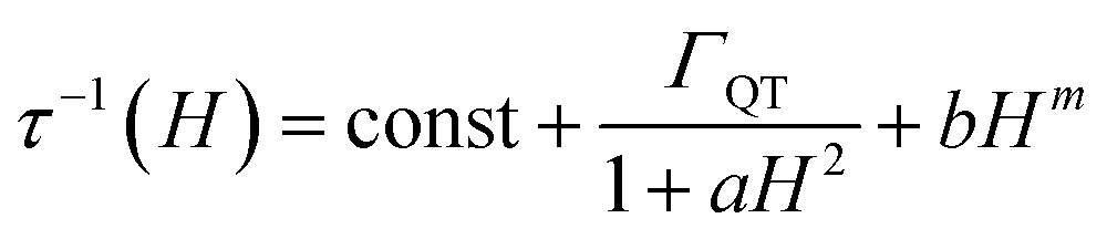 | (3) |
The first term accounts for the Orbach and Raman contributions. The second term considers the suppression of QT by the magnetic field. The field dependence of the direct process is modelled by a phenomenological power law as both D and δ parameters of eqn (2) depend on H. Fixing the Raman, Orbach and QT contributions to the values extracted from the fitting of zero field data in Fig. 3, the three adjustable parameters in the model were: a = 4(4) × 10−5 Oe−2, b = 1(2) × 10−15 s−1 Oe−m for QT and m = 4.1(1) for the direct process.
While the general trend is reproduced, the agreement is rather poor. The reason is that QT accounts for a fraction of the rate (the green bar in Fig. 4) that is much smaller than the decrease we observe on applying the external magnetic field (green plus orange bar in Fig. 4). Therefore, the assumption that the Raman mechanism (the only other relevant contribution at 20 K) is field-independent breaks down. This observation is in line with recent theoretical findings34,36 that the admixing of spin and vibrational states (i.e., the second-order term of the spin-phonon coupling) promotes transitions inside the ground doublet, still requiring the thermal population of the modes. The overall efficiency is temperature dependent due to the occupation of vibrational states but is also field-dependent, as the admixing of the ground doublets depends on the field. However, as soon as the field localizes the two wavefunctions of the ground doublet on opposite sides of the anisotropy barrier, the Raman mechanism becomes field-independent. The unusually large flat region (1–10 kOe) suggests that the Raman mechanism dominates and gives way to the direct process only at high field.
As far as magnetic hysteresis is concerned (Fig. 5 for 1), the behaviour is again very similar to that of the original [Dy(bppen)Cl] derivative, 2. The hysteresis opens below 6 K (100 Oe s−1 sweep rate), and the opening increases on decreasing temperature. The loop is pinched in zero field because of the tunnelling. The dilution in the diamagnetic host only marginally suppresses the zero-field jump in the hysteresis (see Fig. S21† for 1[Y] data).
 | ||
| Fig. 5 Temperature dependence of the hysteresis loops of 1. Field sweeping rate: 100 Oe s−1. | ||
Given that 1 presents all the features of strongly axial SMMs, we also measured the thermomagnetic hysteresis. Zero field cooled (ZFC) and field cooled (FC) magnetization at various fields between 500 and 2500 Oe were measured scanning the temperature at 0.03 K s−1 (see Fig. 6 for 1 at H = 1.6 kOe and Fig. S22 and S23† for more data also on 1[Y]). The curves become irreversible below 3.5 K. Interestingly, the FC curves measured for decreasing and increasing temperatures are not superimposable. The decreasing FC curves cross the ZFC one, but the FC measured on increasing temperatures does not. This behaviour is often reported for well-performing SMMs, including the [Dy(Cpttt)2][B(C6F5)4] system.6
 | ||
| Fig. 6 (a) Experimental and (b) simulated ZFC (blue) and FC (green and red) curves of 1 at a sweeping rate of 0.03 K s−1 and at H = 1.6 kOe. The arrows indicate the direction of the measurement for each curve. | ||
The reason for this crossing, not detected in other SMMs such as the archetypal Mn12 cluster,37 can be ascribed to the fact that the Orbach mechanism is overcome by the Raman process for these lanthanoid-based SMMs. As the relaxation time grows less rapidly on decreasing the temperature, the increase in equilibrium magnetization, which goes approximatively as T−1, cannot be neglected. As a result, the ZFC branch measured on increasing temperature reflects that the configurations with higher equilibrium magnetization have been populated at lower temperatures. A larger magnetization, compared to the FC curve measured on decreasing temperatures, is thus recorded. This is not the case if both the FC and ZFC branches are measured on increasing the temperature.
To further prove this hypothesis, we computed the out-of-equilibrium magnetization by considering the experimental temperature sweeping rate and relaxation times. The relaxation times are those extracted from Fig. 3, while the equilibrium magnetization was estimated by a fourth-order polynomial fit of the experimental data. The only adjustable parameter is the value of the magnetization of the first measured point, which is related to the complex evolution during the field change from zero to the target field. The agreement with the experimental data (see Fig. 6b) is excellent despite the simple model, confirming that the crossing of the curves must be ascribed to the measuring procedure. It is thus recommended that, in the thermomagnetic characterization protocol, an additional in-field branch is measured on increasing the temperature. This will allow an accurate determination and a meaningful comparison of the irreversibility temperature in very anisotropic and well-performing SMMs.
NMR characterization
The magnetic characterization of 1 identifies it as a SMM exhibiting a high anisotropy barrier. Ab initio calculations agree well with the experimental behaviour over a wide temperature and field range. We can thus rely on theory to predict other features that can be of relevance for NMR applications.In this regard, the ab initio computed electronic structure shows strongly axial and collinear g-tensors up to the third Kramers doublet (>1000 K, see Table S8†), suggesting that a large and strongly axial magnetic susceptibility anisotropy will be retained at room temperature in solution. Since the paramagnetic pseudocontact shift is proportional to the magnetic susceptibility anisotropy (vide infra), sizeable pseudocontact shifts are expected up to room temperature.
Starting from the ab initio computed CF parameters, we calculated the principal values of the room temperature magnetic susceptibility tensor (0.0111, 0.0128, and 0.1138 cm3 mol−1). The resulting single-molecule anisotropy is defined as:
 | (4) |
![[small chi, Greek, tilde]](https://www.rsc.org/images/entities/i_char_e11b.gif) ii are the eigenvalues of the magnetic susceptibility tensor, ordered to have zz as the most different from the two other values and xx as the opposite extreme. The estimated Δχax is about 224% of the isotropic magnetic susceptibility (defined as 1/3 of the trace of the tensor: χiso = 9.59 × 10⁻³¹ m3). On the contrary, the rhombic anisotropy, defined as Δχrh =
ii are the eigenvalues of the magnetic susceptibility tensor, ordered to have zz as the most different from the two other values and xx as the opposite extreme. The estimated Δχax is about 224% of the isotropic magnetic susceptibility (defined as 1/3 of the trace of the tensor: χiso = 9.59 × 10⁻³¹ m3). On the contrary, the rhombic anisotropy, defined as Δχrh = ![[small chi, Greek, tilde]](https://www.rsc.org/images/entities/char_e11b.gif) xx − yy = −2.17 × 10⁻³² m3, is less than 3% of the isotropic value. If such a computed large and axial anisotropy is preserved in a fluid solution, it could represent an ideal situation for a solution NMR investigation.
xx − yy = −2.17 × 10⁻³² m3, is less than 3% of the isotropic value. If such a computed large and axial anisotropy is preserved in a fluid solution, it could represent an ideal situation for a solution NMR investigation.
The resolution of the 1H-NMR spectrum of a paramagnetic complex and the observability of shifted signals depend not only on the shifts that the metal ion is able to impart on the probed magnetically active nuclei, but also on how much the presence of the metal centre broadens their lines. In general, nuclear resonances in lanthanoid complexes are only weakly affected by electron-nucleus dipole–dipole relaxation (Solomon relaxation, see eqn (6), (7) and (8) in the Experimental) because the availability of strongly spin–orbit coupled excited states within reach of the phonon distribution at room temperature ensures a fast electron relaxation time. The latter, being short, becomes the correlation time for this nuclear relaxation mechanism, reducing its efficiency.38 However, the nuclear relaxation caused by interaction with the large magnetic moment (the Curie-spin interaction) of the lanthanoid can be impactful. The efficiency of this mechanism depends principally on the molecular weight of the investigated molecule via the molecular reorientation time (eqn (9) and (10) in Methods). The observability of the NMR signal can thus be related to the ratio between the PCS and the transverse relaxation rate caused by the Curie-spin interaction,  , which is proportional to
  .39 Since the isotropic susceptibility mostly depends on the metal ion but not on its coordination environment, Δχax values are already a good indication of the observability of nuclear resonances in different complexes of the same lanthanoid (vide infra). Therefore, it is not surprising that NMR is increasingly included in the characterization of lanthanoid-based SMMs.15,40–46
In Fig. 7 we report the experimental 1H NMR spectrum of 1 recorded at 9.4 T and 293 K in deuterated dichloromethane (further experimental details are given in the Experimental section). The spectrum shows signals with shifts as large as −1200 ppm, with relatively narrow lines. The blue line shows the spectrum calculated using the X-ray determined crystal structure for the scaffold with the hydrogen positions optimized at the DFT level in implicit solvent (see computational details) and the ab initio magnetic susceptibility computed for the molecular structure in the crystalline phase. The parameters used for the simulation are given in the Experimental section.
 | ||
| Fig. 7 Experimental 1H-NMR spectrum of 1 recorded at 293 K and 9.4 T in CD2Cl2 (black) and calculated spectrum (blue). The coloured bars represent calculated positions of the H atoms belonging to the different parts of the molecule (see structure): green = phenol, orange = pyridine, violet = methyl, cyan = aliphatic backbone. For the details of the experiment and simulation see Experimental section. The figure on top of Table S7† reports the ligand alone. The hydrogen atom labelling is based on the Crystallographic Information File (CIF). Symmetry code: (i) 1 − x + 1, y, −z + 3/2. | ||
The calculated spectrum reproduces quite well the experiment, even though the experimental lines appear broader than expected. This is likely due to a conformational exchange phenomenon and additional relaxation due to Fermi contact contribution. The position of the most positively shifted peak, corresponding to the protons of the oxo-benzyl groups, is well reproduced while a slightly larger deviation is observed for the most negatively shifted peak. This is not surprising, as H13 is bound to a carbon atom in α position to the coordinated nitrogen of the pyridine ring. A weak Fermi contact contribution,38 not included in our simulation, might be expected for atoms a few bonds away from the metal centre. The remarkably extensive span of the observed signals (ca. 2200 ppm) is very close to the computed one, demonstrating that the structure is preserved in solution, and so is the axiality of the magnetic susceptibility anisotropy.
This finding is not only relevant for the characterization of this complex and its derivatives but can also have implications exceeding the boundaries of molecular magnetism. For instance, we can compare the PCSs that this complex is able to produce with other prototypical molecules that form the basis of currently used paramagnetic tags. The archetypical dysprosium-based single ion magnet DyDOTA has a computed Δχax = −7.10 × 10⁻³¹ m3. Fig. 8 shows the comparison of the PCS isosurface (±200 ppm) for 1 and DyDOTA superimposed to their molecular structures on the same scale. The value for DyDOTA has been computed from our previous ab initio calculations of its magnetic anisotropy47,48 symmetrizing the computed tensor over four orientations (90° away from each other) around the Dy–Owater bond as expected to occur in a fluid solution (see ESI† for more details). This averaging produces an effective easy-plane anisotropy.
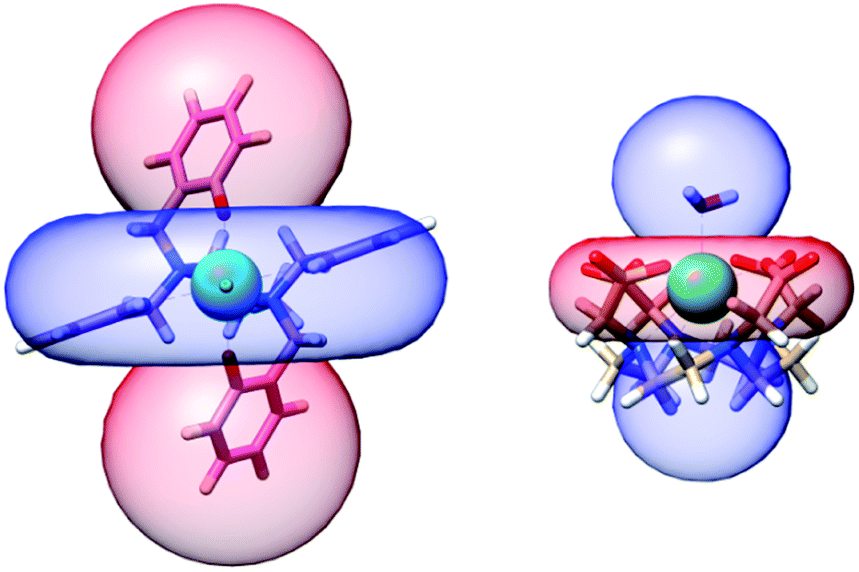 | ||
| Fig. 8 Computed isosurface of pseudocontact shift at ±200 ppm (red – positive, blue – negative) for 1 (left) and DyDOTA (right). The blue and red colours are exchanged in the two complexes due to the different nature of the room temperature magnetic anisotropy. | ||
To better quantify the efficiency of the two complexes as PCS agents, we calculate that a proton along the pseudo C4 axis of DyDOTA experiences an absolute shift of 1 ppm at ca. 23 Å from the metal (ca. 18 Å on the plane). For 1, a 1 ppm shift is obtained at 39 Å for protons along the easy axis (ca. 31 Å in the plane). In other words, grafting an ad hoc functionalized version of 1 to a protein could allow resolving structures at much larger distances from the paramagnetic probe compared to the DOTA- or the even less anisotropic DPA-based tags.17–19
Conclusion
In this article we have reported the synthesis of a new member of a family of pentagonal-bipyramidal Dy-complexes. The relatively simple chemical modification corresponding to the addition of a methyl group in the aliphatic backbone of the ligand has essential effects on magnetic anisotropy as evidenced by ab initio and magnetic studies. The analysis of the relaxation times has evidenced a large window of temperatures and magnetic fields where the Raman relaxation dominates over other thermally activated processes. This feature has allowed us to unequivocally demonstrate that the Raman relaxation mechanism is field-dependent, contrary to what is usually assumed. Moreover, our simulations also show that the crossings between the ZFC and FC curves, often observed in highly performant SMMs but – to the best of our knowledge – never commented, naturally arise from the measuring protocol and the temperature dependence of the relaxation time of these molecules.The remarkable stability of complex 1 also allowed us to record NMR spectra where through-space 1H shifts spanning a range larger than 2000 ppm were observed. This finding, directly related to the huge magnetic anisotropy retained by the complex at room temperature and in solution, opens the possibility to engineer new highly performant PCS tags.
Experimental section
Synthesis
Details on the synthesis, general characterization, and single crystal X-ray diffraction of 1, 4 and 1[Y] are presented as ESI.†Computational details
The hydrogen positions were optimized by density functional theory with ORCA 4.2.1 software.49 The PBE0 functional was employed,50 together with the D3 dispersion correction to account for dispersion forces.51,52 The DKH-def2-TZVP basis sets were used for all atoms53 except for Dy, for which the SARC2-DKH-QZVP basis sets were utilized.54 Conductor-like continuum polarization model was employed to mimic the effect of the CD2Cl2 solvent.55The post-HF calculations of the electronic properties of 1 were carried out with MOLCAS 8.0 quantum chemistry package.56 The calculations were based on the X-ray structure coordinates where only H atoms were optimized. ANO-RCC basis sets57,58 were employed for all atoms: ANO-RCC-VTZP for Dy, O, N and Cl, and ANO-RCC-VDZP for C and H. Scalar relativistic terms were treated by the Douglas–Kroll–Hess Hamiltonian. The calculations were performed at the complete active space self consistent field (CASSCF) level of theory,59 followed by complete active space state interaction by spin–orbit (CASSI-SO).60 The active space consisted of 9 electrons in the 4f orbitals of the Dy atom, CAS(9,7). All the 21 sextuplets of the ground 6H term were computed by state average calculations and included in the following spin–orbit perturbation. Due to limited computational resources, quadruplets and doublets were not computed. The magnitudes and orientations of the magnetic anisotropy axes of the ground and first excited Kramers doublets were mapped with the MOLCAS subroutine SINGLE_ANISO within the pseudospin S = 1/2 approach.61
Magnetic characterization
All the magnetic measurements were performed on pressed pellets of the samples wrapped in Teflon tape. DC measurements and time decays were performed in a SQUID magnetometer. AC magnetic measurements were performed in a Quantum Design Physical Property Measurement System (PPMS). The treatment of the ac data was done with a home-written program in MATLAB language.NMR characterization
The NMR spectrum of 4 was acquired on a Bruker Neo spectrometer operating at 500 MHz 1H Larmor frequency (11.7 T) equipped with a cryogenically cooled probehead.The NMR spectra of 1 were acquired on a Bruker Avance III spectrometer operating at 400 MHz 1H Larmor frequency (9.4 T) to mitigate the field-dependent effects of nuclear spin transverse relaxation. Furthermore, to improve the spectral quality at 5 mm, a 1H selective probe dedicated to paramagnetic systems (the nutation frequency of the hard pulse is ca. 50 kHz) was used. 1H-NMR spectra were acquired on a 400 μmol L−1 solution in CD2Cl2. A pulse of 200 ns was used to excite the entire spectral window. The signal was averaged over a total of ∼4.2 × 10⁶ scans. The baseline was manually corrected over the entire range. To avoid artefacts related to the manual procedure, the presence of signals was evaluated by the circular dispersion of the phase across 512 repetitions of the Fourier-transformed spectrum.62–64
The PCS contribution was calculated from the ab initio magnetic susceptibility tensor and using the point-dipole approximation:65
 | (5) |
 , where the alignment tensor is approximated to the first order as
  .66,67
The above treatment relies on the assumption68,69 of a direct relation between PCS and the magnetic susceptibility tensor, which was recently confirmed by a rigorous quantum chemistry treatment.70
To compute the overall spectrum, the following assumptions were also made: (1) the Fermi contact term is neglected in both the shift and the relaxation;14 (2) the chemical shielding is negligible compared to the paramagnetic contribution and (3) the relaxation due to nucleus–nucleus dipolar coupling and to chemical shielding anisotropy are negligible compared to the paramagnetic contributions.
The linewidth and the intensity of the different 1H resonances were evaluated by computing the relaxation rate as the sum of the dipolar contribution (Solomon term)71 and the part arising from the dipolar shielding anisotropy (Curie-spin term):72,73
| RiM = RSolomoniM + RCurieiM; i = 1, 2 | (6) |
The Solomon terms in R1 and R2 are assumed to be isotropic:
 | (7) |
 | (8) |
On the contrary, the anisotropy of the magnetic susceptibility may result in a sizeable anisotropy in the Curie spin relaxation:42,74–76
 | (9) |
 | (10) |
| Λσ2 = (σxy − σyx)2 + (σxz − σzx)2 + (σyz − σzy)2 |
| Δσ2 = σ2xx + σ2yy + σ2zz − σxxσyy − σxxσzz − σyyσzz + 3/4[(σxy + σyx)2 + (σxz + σzx)2 + (σyz + σzy)2] |
The effect of the finite length of the excitation pulse and the large offsets is accounted for as described in the literature.18 Further details on the calculation of the hyperfine shifts and relaxation parameters are presented in ESI.†
Data availability
All experimental and computed data are available from the authors upon request.Author contributions
The manuscript was written through the contributions of all authors.Conflicts of interest
No conflict of interest to declare.Acknowledgements
Fruitful discussion with Prof. Mauro Botta is gratefully acknowledged. Lila Cadi Tazi is kindly acknowledged for her contribution to the MATLAB program for fitting the ac data. This work has been supported by the Fondazione Cassa di Risparmio di Firenze, by the Italian Ministero dell'Istruzione, dell'Università e della Ricerca through the “Progetto Dipartimenti di Eccellenza 2018–2022 ref. 96C1700020008”, the Department of Chemistry “Ugo Schiff” of the University of Florence, and by the University of Florence through the “Progetti Competitivi per Ricercatori”. ER acknowledges the support and the use of resources of Instruct-ERIC, a landmark ESFRI project, and specifically the CERM/CIRMMP Italy center. GP gratefully acknowledges FAPERJ (through grants E-26/202.912/2019, SEI-260003/001167/2020 and E-26/010.000978/2019) for the financial support. FSS, MB and JFS are grateful to Brazilian CNPq (Conselho Nacional de Desenvolvimento Científico e Tecnológico, grants 308426/2016-9 and 314581/2020-0), CAPES (Coordenação de Aperfeiçoamento de Pessoal de Nível Superior, Finance Code 001) and PrInt/CAPES-UFPR Internationalization Program.References
- S. Gómez-Coca, D. Aravena, R. Morales and E. Ruiz, Coord. Chem. Rev., 2015, 289, 379–392 CrossRef.
- M. Perfetti and J. Bendix, Inorg. Chem., 2019, 58, 11875–11882 CrossRef CAS PubMed.
- M. A. Sørensen, U. B. Hansen, M. Perfetti, K. S. Pedersen, E. Bartolomé, G. G. Simeoni, H. Mutka, S. Rols, M. Jeong, I. Zivkovic, M. Retuerto, A. Arauzo, J. Bartolomé, S. Piligkos, H. Weihe, L. H. Doerrer, J. van Slageren, H. M. Rønnow, K. Lefmann and J. Bendix, Nat. Commun., 2018, 9, 1292 CrossRef.
- Y. S. Ding, N. F. Chilton, R. E. Winpenny and Y. Z. Zheng, Angew. Chem., 2016, 128, 16305–16308 CrossRef.
- F.-S. Guo, B. M. Day, Y.-C. Chen, M.-L. Tong, A. Mansikkamäki and R. A. Layfield, Science, 2018, 362, 1400–1403 CrossRef CAS PubMed.
- C. A. Goodwin, F. Ortu, D. Reta, N. F. Chilton and D. P. Mills, Nature, 2017, 548, 439–442 CrossRef CAS PubMed.
- S. T. Liddle and J. van Slageren, Chem. Soc. Rev., 2015, 44, 6655 RSC.
- E. Ravera, A. Carlon, M. Fragai, G. Parigi and C. Luchinat, Emerging Top. Life Sci., 2018, 2, 19–28 CrossRef CAS.
- T. Müntener, D. Joss, D. Häussinger and S. Hiller, Chem. Rev., 2022 DOI:10.1021/acs.chemrev.1c00796.
- Q. Miao, C. Nitsche, H. Orton, M. Overhand, G. Otting and M. Ubbink, Chem. Rev., 2022 DOI:10.1021/acs.chemrev.1c00708.
- L. Gigli, S. Di Grande, E. Ravera, G. Parigi and C. Luchinat, Magnetochemistry, 2021, 7, 96 CrossRef CAS.
- V. V. Novikov, A. A. Pavlov, A. S. Belov, A. V. Vologzhanina, A. Savitsky and Y. Z. Voloshin, J. Phys. Chem. Lett., 2014, 5, 3799–3803 CrossRef CAS PubMed.
- J. A. Peters, K. Djanashvili, C. F. Geraldes and C. Platas-Iglesias, Coord. Chem. Rev., 2020, 406, 213146 CrossRef CAS.
- D. Parker, E. A. Suturina, I. Kuprov and N. F. Chilton, Acc. Chem. Res., 2020, 53, 1520–1534 CrossRef CAS PubMed.
- M. Damjanović, Y. Horie, T. Morita, Y. Horii, K. Katoh, M. Yamashita and M. Enders, Inorg. Chem., 2015, 54, 11986–11992 CrossRef.
- Z. Liang, M. Damjanovic, M. Kamila, G. Cosquer, B. K. Breedlove, M. Enders and M. Yamashita, Inorg. Chem., 2017, 56, 6512–6521 CrossRef CAS PubMed.
- D. Joss and D. Häussinger, Prog. Nucl. Magn. Reson. Spectrosc., 2019, 114, 284–312 CrossRef PubMed.
- C. Nitsche and G. Otting, Paramagnetism in Experimental Biomolecular NMR, 2018, 16, 42 CAS.
- W.-M. Liu, M. Overhand and M. Ubbink, Coord. Chem. Rev., 2014, 273, 2–12 CrossRef.
- Z. Zhu, C. Zhao, T. Feng, X. Liu, X. Ying, X.-L. Li, Y.-Q. Zhang and J. Tang, J. Am. Chem. Soc., 2021, 143, 10077–10082 CrossRef CAS PubMed.
- Z. Zhu, C. Zhao, Q. Zhou, S. Liu, X.-L. Li, A. Mansikkamäki and J. Tang, CCS Chem., 2022, 1–24 Search PubMed.
- J. Liu, Y.-C. Chen, J.-L. Liu, V. Vieru, L. Ungur, J.-H. Jia, L. F. Chibotaru, Y. Lan, W. Wernsdorfer, S. Gao, X.-M. Chen and M.-L. Tong, J. Am. Chem. Soc., 2016, 138, 5441–5450 CrossRef CAS PubMed.
- Z. Jiang, L. Sun, Q. Yang, B. Yin, H. Ke, J. Han, Q. Wei, G. Xie and S. Chen, J. Mater. Chem. C, 2018, 6, 4273–4280 RSC.
- L. E. d. N. Aquino, G. A. Barbosa, J. d. L. Ramos, S. O. K. Giese, F. S. Santana, D. L. Hughes, G. G. Nunes, L. Fu, M. Fang, G. Poneti, A. N. Carneiro Neto, R. T. Moura Jr, R. A. S. Ferreira, L. D. Carlos, A. G. Macedo and J. F. Soares, Inorg. Chem., 2021, 60, 892–907 CrossRef CAS PubMed.
- T. Gregório, J. d. M. Leão, G. A. Barbosa, J. d. L. Ramos, S. O. K. Giese, M. Briganti, P. C. Rodrigues, E. L. de Sá, E. R. Viana, D. L. Hughes, L. D. Carlos, R. A. Ferreira, A. G. Macedo, G. G. Nunes and J. F. Soares, Inorg. Chem., 2019, 58, 12099–12111 CrossRef PubMed.
- J. C. Ott, E. A. Suturina, I. Kuprov, J. Nehrkorn, A. Schnegg, M. Enders and L. H. Gade, Angew. Chem., 2021, 133, 23038–23046 CrossRef.
- J. Sievers, Z. Phys. B: Condens. Matter, 1982, 45, 289–296 CrossRef CAS.
- J. D. Rinehart and J. R. Long, Chem. Sci., 2011, 2, 2078–2085 RSC.
- R. D. Shannon, Acta Crystallogr., Sect. A: Cryst. Phys., Diffr., Theor. Gen. Crystallogr., 1976, 32, 751–767 CrossRef.
- E. Wong, S. Liu, S. Rettig and C. Orvig, Inorg. Chem., 1995, 34, 3057–3064 CrossRef CAS.
- Y. Yamada, S.-I. Takenouchi, Y. Miyoshi and K.-I. Okamoto, J. Coord. Chem., 2010, 63, 996–1012 CrossRef CAS.
- E. Ravera, L. Gigli, B. Czarniecki, L. Lang, R. Kümmerle, G. Parigi, M. Piccioli, F. Neese and C. Luchinat, Inorg. Chem., 2021, 60, 2068–2075 CrossRef PubMed.
- B. Yin and C.-C. Li, Phys. Chem. Chem. Phys., 2020, 22, 9923–9933 RSC.
- M. Briganti, F. Santanni, L. Tesi, F. Totti, R. Sessoli and A. Lunghi, J. Am. Chem. Soc., 2021, 143, 13633–13645 CrossRef CAS PubMed.
- J. M. Zadrozny, M. Atanasov, A. M. Bryan, C.-Y. Lin, B. D. Rekken, P. P. Power, F. Neese and J. R. Long, Chem. Sci., 2013, 4, 125–138 RSC.
- A. Lunghi and S. Sanvito, J. Chem. Phys., 2020, 153, 174113 CrossRef CAS PubMed.
- R. Sessoli, D. Gatteschi, A. Caneschi and M. A. Novak, Nature, 1993, 365, 141–143 CrossRef CAS.
- I. Bertini, C. Luchinat, G. Parigi and E. Ravera, NMR of Paramagnetic Molecules: applications to metallobiomolecules and models, Elsevier, Amsterdam, NL, 2015 Search PubMed.
- C. Geraldes and C. Luchinat, Met. Ions Biol. Syst., 2003, 40, 513–588 CAS.
- M. Vonci, K. Mason, E. A. Suturina, A. T. Frawley, S. G. Worswick, I. Kuprov, D. Parker, E. J. McInnes and N. F. Chilton, J. Am. Chem. Soc., 2017, 139, 14166–14172 CrossRef CAS PubMed.
- A. C. Harnden, E. A. Suturina, A. S. Batsanov, P. K. Senanayake, M. A. Fox, K. Mason, M. Vonci, E. J. McInnes, N. F. Chilton and D. Parker, Angew. Chem., 2019, 131, 10396–10400 CrossRef.
- E. A. Suturina, K. Mason, C. F. Geraldes, N. F. Chilton, D. Parker and I. Kuprov, Phys. Chem. Chem. Phys., 2018, 20, 17676–17686 RSC.
- N. Ishikawa, T. Iino and Y. Kaizu, J. Phys. Chem. A, 2002, 106, 9543–9550 CrossRef CAS.
- M. Damjanovic, K. Katoh, M. Yamashita and M. Enders, J. Am. Chem. Soc., 2013, 135, 14349–14358 CrossRef CAS PubMed.
- M. Hiller, S. Krieg, N. Ishikawa and M. Enders, Inorg. Chem., 2017, 56, 15285–15294 CrossRef CAS PubMed.
- M. Sugita, N. Ishikawa, T. Ishikawa, S.-y. Koshihara and Y. Kaizu, Inorg. Chem., 2006, 45, 1299–1304 CrossRef CAS.
- M. Briganti, E. Lucaccini, L. Chelazzi, S. Ciattini, L. Sorace, R. Sessoli, F. Totti and M. Perfetti, J. Am. Chem. Soc., 2021, 143, 8108–8115 CrossRef CAS PubMed.
- M. Briganti, G. F. Garcia, J. Jung, R. Sessoli, B. Le Guennic and F. Totti, Chem. Sci., 2019, 10, 7233–7245 RSC.
- F. Neese, Wiley Interdiscip. Rev.: Comput. Mol. Sci., 2018, 8, e1327 Search PubMed.
- C. Adamo and V. Barone, J. Chem. Phys., 1999, 110, 6158–6170 CrossRef CAS.
- S. Grimme, J. Antony, S. Ehrlich and H. Krieg, J. Chem. Phys., 2010, 132, 154104 CrossRef PubMed.
- S. Grimme, S. Ehrlich and L. Goerigk, J. Comput. Chem., 2011, 32, 1456–1465 CrossRef CAS PubMed.
- F. Weigend and R. Ahlrichs, Phys. Chem. Chem. Phys., 2005, 7, 3297–3305 RSC.
- D. Aravena, F. Neese and D. A. Pantazis, J. Chem. Theory Comput., 2016, 12, 1148–1156 CrossRef CAS PubMed.
- V. Barone and M. Cossi, J. Phys. Chem. A, 1998, 102, 1995–2001 CrossRef CAS.
- F. Aquilante, J. Autschbach, R. K. Carlson, L. F. Chibotaru, M. G. Delcey, L. De Vico, I. F. Galván, N. Ferré, L. M. Frutos, L. Gagliardi, M. Garavelli, A. Giussani, C. E. Hoyer, G. Li Manni, H. Lischka, D. Ma, P. Å. Malmqvist, T. Müller, A. Nenov, M. Olivucci, T. B. Pedersen, D. Peng, F. Plasser, B. Pritchard, M. Reiher, I. Rivalta, I. Schapiro, J. Segarra-Martí, M. Stenrup, D. G. Truhlar, L. Ungur, A. Valentini, S. Vancoillie, V. Veryazov, V. P. Vysotskiy, O. Weingart, F. Zapata and R. Lindh, J. Comput. Chem., 2016, 37, 506–541 CrossRef CAS PubMed.
- B. O. Roos, R. Lindh, P.-Å. Malmqvist, V. Veryazov and P.-O. Widmark, J. Phys. Chem. A, 2004, 108, 2851–2858 CrossRef CAS.
- B. r. O. Roos, R. Lindh, P.-Å. Malmqvist, V. Veryazov, P.-O. Widmark and A. C. Borin, J. Phys. Chem. A, 2008, 112, 11431–11435 CrossRef CAS.
- B. O. Roos and P.-Å. Malmqvist, Phys. Chem. Chem. Phys., 2004, 6, 2919–2927 RSC.
- P. A. Malmqvist, B. O. Roos and B. Schimmelpfennig, Chem. Phys. Lett., 2002, 357, 230–240 CrossRef CAS.
- L. F. Chibotaru and L. Ungur, J. Chem. Phys., 2012, 137, 064112 CrossRef CAS PubMed.
- J. Fukazawa and K. Takegoshi, Phys. Chem. Chem. Phys., 2010, 12, 11225–11227 RSC.
- J. Fukazawa, K. Takeda and K. Takegoshi, J. Magn. Reson., 2011, 211, 52–59 CrossRef CAS PubMed.
- E. Ravera, J. Magn. Reson., 2021, 100022 CrossRef.
- R. J. Kurland and B. R. McGarvey, J. Magn. Reson., 1970, 2, 286–301 CAS.
- J. Lohman and C. MacLean, Chem. Phys., 1978, 35, 269–274 CrossRef CAS.
- C. Gayathri, A. Bothner-By, P. Van Zijl and C. Maclean, Chem. Phys. Lett., 1982, 87, 192–196 CrossRef CAS.
- L. Cerofolini, J. M. Silva, E. Ravera, M. Romanelli, C. F. Geraldes, A. L. Macedo, M. Fragai, G. Parigi and C. Luchinat, J. Phys. Chem. Lett., 2019, 10, 3610–3614 CrossRef CAS PubMed.
- G. Parigi, L. Benda, E. Ravera, M. Romanelli and C. Luchinat, J. Chem. Phys., 2019, 150, 144101 CrossRef PubMed.
- L. Lang, E. Ravera, G. Parigi, C. Luchinat and F. Neese, J. Phys. Chem. Lett., 2020, 11, 8735–8744 CrossRef CAS PubMed.
- I. Solomon, Phys. Rev., 1955, 99, 559 CrossRef CAS.
- M. Guéron, J. Magn. Reson., 1975, 19, 58–66 Search PubMed.
- A. J. Vega and D. Fiat, Mol. Phys., 1976, 31, 347–355 CrossRef CAS.
- N. Bloembergen, J. Chem. Phys., 1957, 27, 572–573 CrossRef CAS.
- G. Parigi, E. Ravera and C. Luchinat, Prog. Nucl. Magn. Reson. Spectrosc., 2019, 114, 211–236 CrossRef PubMed.
- R. M. Gregory and A. D. Bain, Concepts Magn. Reson., Part A, 2009, 34, 305–314 CrossRef.
Footnotes |
| † Electronic supplementary information (ESI) available: Synthetic procedures and crystallographic characterization. Magnetic measurements and simulations. Energy level structure and composition. Computational details. NMR details. CCDC 2129444 (complex 1) and 2129445 (complex 4). For ESI and crystallographic data in CIF or other electronic format see https://doi.org/10.1039/d2sc01619b |
| ‡ These authors contributed equally. |
| This journal is © The Royal Society of Chemistry 2022 |