 Open Access Article
Collective variable discovery in the age of machine learning: reality, hype and everything in between†‡
Soumendranath Bhakat *
*
Department of Biochemistry and Biophysics, Perelman School of Medicine, University of Pennsylvania, Pennsylvania 19104-6059, USA. E-mail: bhakatsoumendranath@gmail.com; Tel: +1 30549 32620
First published on 2nd September 2022
Abstract
Understanding the kinetics and thermodynamics profile of biomolecules is necessary to understand their functional roles which has a major impact in mechanism driven drug discovery. Molecular dynamics simulation has been routinely used to understand conformational dynamics and molecular recognition in biomolecules. Statistical analysis of high-dimensional spatiotemporal data generated from molecular dynamics simulation requires identification of a few low-dimensional variables which can describe the essential dynamics of a system without significant loss of information. In physical chemistry, these low-dimensional variables are often called collective variables. Collective variables are used to generate reduced representations of free energy surfaces and calculate transition probabilities between different metastable basins. However the choice of collective variables is not trivial for complex systems. Collective variables range from geometric criteria such as distances and dihedral angles to abstract ones such as weighted linear combinations of multiple geometric variables. The advent of machine learning algorithms led to increasing use of abstract collective variables to represent biomolecular dynamics. In this review, I will highlight several nuances of commonly used collective variables ranging from geometric to abstract ones. Further, I will put forward some cases where machine learning based collective variables were used to describe simple systems which in principle could have been described by geometric ones. Finally, I will put forward my thoughts on artificial general intelligence and how it can be used to discover and predict collective variables from spatiotemporal data generated by molecular dynamics simulations.
1 Introduction
Over the past three decades, the major focus of structural biology and biophysics has been to understand the conformational dynamics of biological systems across a broad range of timescales with high spatial resolution (ability to visualise molecular motion). Molecular dynamics (MD) simulation acts as a computational microscope which can capture biologically relevant conformational dynamics across varied timescales with high spatial resolution.1 Major advances in computational hardware and algorithms led to an ever-growing use of MD simulation in varied biological systems. A typical MD simulation generates high-dimensional spatiotemporal data which captures complex molecular motions. Simulation of increasingly larger molecules at ever increasing time scales leads to the ‘curse of dimensionality’ which can be summarised as follows: “as the size of the biomolecule and the simulation length increases, it also increases the number of explanatory temporal variables (e.g. H-bond distances, radius of gyration, RMSD, dihedral angles etc.) and the problem of structure discovery using temporal variables gets harder. This is analogous to the problem of variable selection during model fitting in machine learning.2”Capturing low-dimensional representation (without significant loss of information regarding slow conformational degrees of freedom) from high-dimensional temporal data is an open area of research in biomolecular simulation. An excellent example of this is the large scale flap dynamics in plasmepsin-II and BACE-1.3 In plasmepsin-II, the sine/cos transformation of χ1 and χ2 angles of 20 residues present in the flap region generates 58 dimensions. Such a high number of dimensions makes it incredibly difficult to capture slow degrees of freedom which dominate flap opening. However, careful analysis of the probability distributions showed that flipping of χ1 and χ2 angles of conserved tyrosine (Tyr) governs the flap dynamics in plasmepsin-II and BACE-1.4 Such low-dimensional projections which best captures the conformational changes are known as collective variables (CVs) or order parameters (not to be confused with NMR order parameter which is a measure of conformational entropy). Temporal evolution along CVs provide thermodynamic and kinetic informations about conformational changes.5–7 It is worth mentioning that the use of buzz-word “automatic identification” to highlight new methods for CV discovery from MD simulation gives a false impression i.e. selection of good CV is a streamlined and well-defined process. But in practice, naive application of automated methods leads to uninterpretable and poor choice of CVs. Further such methods are not necessarily new, but in most cases direct applications or minor modifications of machine learning algorithms developed for classification (binary classifiers and their variants), signal processing (PCA, TICA, autoencoders etc), time-series prediction (neural networks, hidden Markov model etc.) and natural language processing (LSTM, transformers) etc. Recent years saw a sharp rise in applying machine learning algorithms for CV selection on systems which can be represented by simple geometric CVs e.g. dihedral angles, H-bond, RMSDs etc (highlighted in later sections).
Due to overuse of the words ‘AI/machine learning’ and flood of papers reporting new algorithms, the current field of CV discovery in biomolecular simulation is hard to navigate for a beginner or people from other disciplines. In this review we will classify the CV discovery process as following: (1) geometric (dihedral angles, H-bonds, RMSD etc) and (2) abstract (PCA, ICA, neural network etc.). One question that is still up in the air: “Has the field of CV discovery in biomolecular simulation reached a plateau?”. I will provide my opinion on the aforementioned question and will put forward some challenges in order to the test the robustness and general applicability of CV discovery algorithms in context of biomolecular simulation.
2 Metastability & collective variables
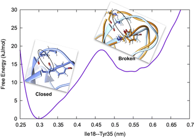
Before we dive into the definition of CV, we must understand the concept of metastability. Let's consider basic pancreatic trypsin inhibitor (BPTI) as an example and focus on a particular H-bond between Ile18–N–O–Tyr35 (Fig. 1). In crystal conformation the aforementioned H-bond remains in a closed conformation. If one performs a short MD simulation, the stationary probability distribution fluctuates around the closed basin, however, careful analysis of 1 ms MD simulation showed formation of broken conformations. A CV (in this case the H-bond distance) should be able to distinguish the metastable states (such as broken and closed conformations) and estimate apparent free energy profile along it as described by following equation:
F(x) = −kBT![[thin space (1/6-em)]](https://www.rsc.org/images/entities/char_2009.gif) ln ln![[thin space (1/6-em)]](https://www.rsc.org/images/entities/char_2009.gif) P(x) P(x)
| (1) |
The rugged nature of biomolecular energy landscape is by definition characterised by numerous metastable basins. An optimal CV is the one for which two metastable states are separated by high free energy barrier (Fig. 2). In most cases a single CV is not enough to capture the complexity of conformational landscape. Selection of CVs is an essential step to perform free energy/kinetics calculations and drive pathway based sampling methods e.g. metadynamics,8 steered MD,9 umbrella sampling10 etc.
For the sake of simplicity CVs can be divided into two categories: (1) geometric and (2) abstract.
2.1 Geometric CVs
Most commonly used geometric CVs that captures conformational dynamics in biomolecules are:(a) Distance: in biomolecular simulation two kinds of distances are most commonly used:
(i) distance between two atoms
(ii) distance between center of mass (COM) of two group of atoms.
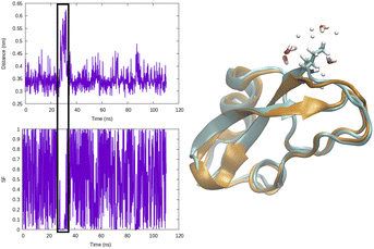
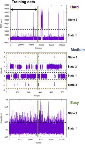
Distance as CVs can be used as an input within adaptive sampling and enhanced sampling methods. For example, distance between COM of ligand and protein can be used as a CV to capture ligand unbinding using well-tempered metadynamics.4,11 Similarly H-bond distance can be used as CV (Fig. 3) to capture transition between closed and broken states. Such CV can be especially useful to study transient solvent exposure in protein which leads to hydrogen–deuterium exchange (paper in preparation).
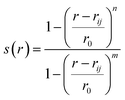
(b) Switching function: a smoother version of distance CV is switching function (SF) which allows a smoother transition between two metastable states along a particular distance (Fig. 3). A typical mathematical form (other functional forms of switching function includes tanh, Gaussian, exponential, cubic etc) of SF can be described as follows:
 | (2) |
A more general CV which combines multiple distances with switching function is known as contact map. It calculates the distances between a number of pairs of atoms and convert each distance by a switching function. Such CVs are useful where fluctuation along multiple distances governs conformational dynamics.
(c) Dihedral angle: tracking temporal evolution of dihedral angles (e.g. ϕ, ψ, ω, χ1, χ2) during MD simulation is a well established method to capture conformational dynamics of biomolecules. Most common example includes tracking the conformational sampling in alanine dipeptide by probability distribution along ϕ and ψ angles. Recently, Bhakat and Söderhjelm4 showed that the conformational dynamics of pepsin-like aspartic proteases can be captured by two dihedral angles: χ1 and χ2 angles of conserved Tyr (Fig. 4 highlights evolution of χ1 during MD simulation). However in many cases, conformational dynamics of biomolecules can't be captured by a few dihedral angles. In complex cases, linear combinations of dihedral angles (more on this later) can be used as CVs to capture biomolecular dynamics.
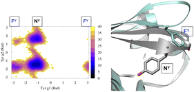 | ||
| Fig. 4 Projection of χ1 and χ2 angle of Tyr77 in apo plasmepsin-II (PDB: 1LF4) during unbiased ∼600 ns long MD simulation (left panel). Tyr77 predominantly remains in the normal state (NY) with rare sampling of the flipped state (FY). Conformational snapshots corresponding normal and flipped states with relative position of flap (β hairpin structure) is also highlighted (right panel). In apo plasmepsin-II, rotation of Tyr77 along χ1 and χ2 angles dictates the extent of flap opening which governs substrate entry and catalytic activity. | ||
(d) RMSD: RMSD is one of the commonly used CV which measures the similarity between two superimposed atomic co-ordinates. RMSD is the measure of average distance and in bimolecular simulation it measures deviation of atomic co-ordinates from the starting conformation using the following equation:
 | (3) |
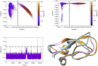 | ||
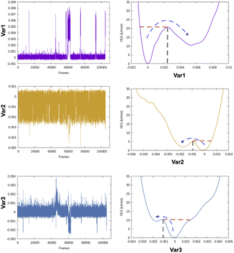
| Fig. 5 Projection of different variables (more precisely time independent components as described in Fig. 8) which captures transient loop opening BPTI as a function of Cα RMSD of residue 6–56 in BPTI. It can be easily seen that a higher RMSD value separates two metastable states along variable 1. Snapshots corresponding crystal (orange), RMSD ∼0.15 nm (pink) and RMSD ∼ 0.25 nm (sea green) highlights differences in loop conformation. RMSD calculation was performed on M1 state13 of 1 ms long conventional MD simulation performed by D. E. Shaw Research.14 | ||
Besides the aforementioned CVs, several other geometric variables (radius of gyration, eRMSD) are frequently used to analyse MD simulations. Softwares e.g. Plumed,15 gmx plugins integrated with Gromacs, CPPTRAJ,16 MDAnalysis,17 MDTraj18 have build-in capabilities to perform analysis of MD trajectories using geometric CVs.
2.2 Abstract CVs
Abstract CVs are usually linear or non-linear transformations of geometric CVs (e.g. dihedral angles, distances, RMSD etc). However the former is often less intuitive compared to the latter. In case of linear transformation, the transformed data is a linear combination of original variables. Whereas non-linear transformations are more complex than that. In this section, I will underscore some of abstract CVs (linear: principal component analysis & independent component analysis; non-linear: kernel trick, diffusion map, t-SNE) that have been regularly used to capture low-dimensional spatiotemporal representation from high dimensional dataset generated by MD simulation. I will further discuss the probabilistic interpretation of variational autoencoders which has been applied to capture compressed representation of temporal variables from molecular simulation. Finally, I will highlight the application of binary classifiers in context of classifying metastable states and drive enhanced sampling simulations to capture state transitions. I will further list the softwares/tools/codes that can be used to generate abstract CVs in context of biomolecular simulation. be a vector of geometric CVs e.g. dihedral angles or distances (assuming r is mean free). First principal component (PC1) of the dataset r1, r2, r3, …, rN is the weighted linear combination of the features that captures the largest variance:
| y1 = w11r1 + w21r2 + w31r3 + … + wN1rN | (4) |
 . The process of generating PCs can be summarised as follows:
(a) generate a mean free version of the input data i.e. a vector of geometric CVs
(b) compute eigenvectors and eigenvalues from the covariance matrix
 | (5) |
(c) sort the eigenvalues in descending order and retain k (k is the new subspace k < D) eigenvectors that corresponds to k largest eigenvalues. The eigenvector corresponds to the largest eigenvalue capture the greatest variability in the data.
(d) construct a projection matrix w with elements w1j, w2j, wNj (where w = [w1j,w2j, …, wNj]T).
(e) generate the PCs, y by transforming the original geometric vectors r via elements of the projection matrix w.
Principal components are uncorrelated to each other (as eigenvectors are orthogonal to one another) and sorted by their variance (PC1 > PC2 > PC3…). PCs extracted from MD dataset defines direction in feature space along maximal variance (largest amplitude/fluctuations). PCA has been applied routinely on periodic (dihedral angles) and non-periodic (CA atomic positions, RMSDs, distances) degrees of freedom (Fig. 6). The coefficients w corresponding each variables allows incorporating PCs as CVs within enhanced sampling protocols e.g. metadynamics and its variants. PCA reduced dimensions can be also used to construct free energy surface of biomolecules. Despite its success, application of PCA in biomolecular simulation has been a subject of controversy. It has been argued that PCA can't capture the slow conformational degrees of freedom within time scales accessible to MD simulations. However, the author believes that PCA on a carefully chosen subset of atomic co-ordinates can capture slow conformational changes in biomolecules.
Softwares: MDAnalysis, Plumed (with capability of using PCs as CVs in metadynamics), MSMBuilder,20 PyEMMA,21 pytraj, scikit-learn (can't be directly used on MD trajectories but can be interfaced with MD post-processing tools e.g. MDTraj).
| p(y1(t),y2(t)) = p(y1(t))p(y2(t)) | (6) |
| Cr(τ) = <r(t)r(t + τ)T> | (7) |
 | (8) |
Symmetrization is a mathematical trick which allows applying the algorithm to the reversible dynamics (as 〈r(t + τ)r(t)T〉 = 〈r(t)r(t − τ)T〉). It also makes sure that the eigenvalues are real and two eigenvectors that comes from distinct eigenvalues are orthogonal. Finally the TICA problem can be formulated a generalised eigenvalue problem (can be solved by second-order blind source separation algorithms e.g. AMUSE):
| Cr(τ)A = Cr(0)AΛ | (9) |
| λ1 < λ2 < … <λN; λ1 captures largest auto-covariance and so on | (10) |
The eigenvalues, λi are associated with the relaxation timescales of a biomolecular process by:
 | (11) |
TICA has been routinely used on temporal data from MD simulation to identify slow conformational degrees of freedom such as flipping of side-chain dihedral angle (Fig. 7), transient exposure of protein interior which leads of solvent exposure (Fig. 8) and drive enhanced sampling simulations.25 Recently Schultze and Grubmuller compared projection of TICs between high-dimensional data from protein dynamics and random walk.26 However the authors disregarded any discussion surrounding the choice of input features and its effect on TICA. Fig. 7 highlights the importance of input features in describing conformational dynamics along TIC space. Lack of separation aka population gap along TIC space in ref. 26 (see Fig. 7, left panel) is a sign that either TICA analysis was performed on a poorly chosen feature space or the sampling was not sufficient enough to capture slow conformational dynamics in proteins.
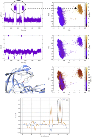 | ||
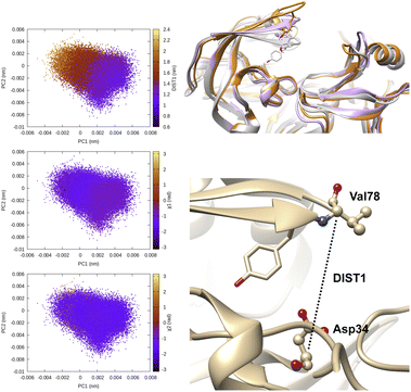
| Fig. 7 Evolution of χ1 and χ2 angles of Tyr77 of plasmepsin-II during MD simulation. TICA analysis (lag time 10 ns) was performed on χ1 and χ2 angles (sin/cos modification) of residue 74–84. Projection of TIC1 and TIC2 along χ1 and χ2 angles of Tyr77 shows that TIC1 managed to capture the slowest degree of motion which is the χ2 rotation of Ty77. Further, projection along TICs failed to separate fluctuation along DIST1 as it is defined by distance between backbone Cα atoms. Fluctuation of TIC coefficients (eigenvalues) also highlights feature no 21 (sin χ2 of Tyr77) as the dominant feature among 25 features (Table 1 in ESI‡). Snapshots corresponding crystal (grey) and flipped (χ2 ∼ 2 rad) are also highlighted. | ||
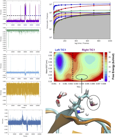 | ||
| Fig. 8 Time-series projection of first 5 TICs and corresponding implied timescales showing how first few TICs captured slow conformational degrees of freedom (transient loop opening as depicted in Fig. 5) in BPTI. TICA analysis was performed on Cα atomic positions of residues 6–56 using a lag time of 500 frames (all calculations were performed on M1 state as described by ref. 13). Transient loop opening in BPTI leads to breaking of H-bond interaction between Ile18–NH and Tyr35–O which makes the amide of Ile18 solvent exposed and enables hydrogen–deuterium exchange.29 Projection of water distance from Ile18–NH shows how TIC1 captures a metastable solvent exposed basin where a water molecule comes within 0.25 nm of amide hydrogen. Snapshot corresponding solvent exposed conformation highlights the relative position of backbone amide and closest (with 0.3 nm) waters. | ||
Wiskott and co-workers27 have shown how the objective function of TICA with lag time 1 is formally equivalent to slow feature analysis (SFA) which captures slowly varying features from high-dimensional data (Fig. 9). SFA and TICA are based on two different principles: slowness and statistical independence. However, the similarity between SFA and TICA (second order ICA with lag-time 1) opens up possibilities to combine these two algorithms28 for capturing slowly varying statistically independent components from high-dimensional temporal data generated by MD simulation.
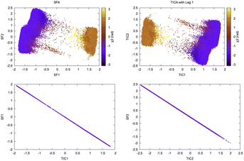 | ||
| Fig. 9 Projection of slow features and TICs with lag time 1 along χ2 angle of Tyr77 shows similarity of TICA and SFA in separating slow conformational degree of freedom. The squared Pearson correlation coefficient, R2 between SFA and TICA with lag time 1 is 1.00. This example is a demonstration of mathematical concepts described in ref. 27 in context of biomolecular simulation. It further raises possibilities of combining the two algorithms and use it to develop Markov state model. | ||
Softwares: MSMBuilder,20 PyEMMA21 and deeptime30 comes with built in TICA functionality. A scikit-learn style implementation of SFA can be found here: https://github.com/wiskott-lab/sklearn-sfa.
 , kernel function k(ri, rj) generates modified inner products which maps
 | (12) |
 must be proper inner product. One doesn't need to explicitly compute ϕ as the kernel matrix k(ri, rj) (modified inner product) can be easily computed by a variety of functions:
(a) Polynomial kernel: k(ri,rj) = (γ·rTirj + c)d, γ > 0
(b) Sigmoid kernel: k(ri,rj) = tanh(γ.rTirj + r).
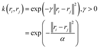
(c) Gaussian kernel: k(ri,rj) = exp(−γ·‖ri − rj‖2), γ > 0. where r, d and γ are kernel hyper-parameters. A drawback of this approach is that when we map the data into higher dimensions, we may overfit the model. Hence the choice of right kernel functions are of utmost importance. Schwartz and colleagues used kernel PCA (using polynomial kernel function) to identify CVs in lactate dehydrogenase. Further, kernel TICA has been used to identify CVs which captures folded to unfolded transition in small folded proteins.32
Softwares: scikit-learn and MODE-TASK33 have in-built kernel PCA functionality. MSMBuilder has a built in kernel TICA algorithm which can be applied on high-dimensional features from MD dataset for discovering low-dimensional representations aka CVs.
In a random walk Markov model the connectivity between data points ri and rj is defined as the probability of jumping from state ri to rj in one step of random walk. The connectivity can be also expressed as a normalised kernel function k(ri, rj) (similar to the functional form of Gaussian kernel. One can choose other measures of distances as kernel functions e.g. Mahalonibis distance, Jensen–Shannon divergence etc.) which measures similarity between data points:
 | (13) |
(a) k is symmetric: k(ri, rj) = k(rj, ri). This allows spectral analysis of the distance matrix kij
(b) k(ri, rj) ≥ 0.
The transition probability p(ri, rj) can be expressed as:
 | (14) |
| PA = ΛA | (15) |
| A(r) = (λt1a1(r),λt2a2(r), …, λtka1(r)) | (16) |
The diffusion distance (analogous to the functional form of kinetic distance as proposed by Noe and Clementi ref. 34) at time t can be expressed as a function of eigenvectors. Kevrekidis and coworkers35 has shown that the diffusion distance can be approximated as Euclidean distance on the diffusion map space:
 | (17) |
Eqn (16) provides justification of using Euclidean distance in the diffusion map space for clustering. Diffusion distance can also be interpreted as a measure of how kinetically close are the two conformations. The distance is small if there are multiple high probability transition pathways between two conformations. Diffusion map has been applied in biomolecular simulation to capture slow transitions and guide enhanced sampling simulations.36–38 Recently the functional form of eqn (16) in combination with maximum entropy based CV selection method SGOOP was used to capture kinetically relevant low dimensional projection in small peptides.39
Softwares: MDAnalysis has an integrated diffusion map module which can be applied on selected features from MD simulation.
 | (18) |
 | (19) |
The Gaussian bandwidth σi has been set in such a way that the perplexity of the conditional distribution equals to the perplexity provided by the user (40 highlighted that there is a monotonically increasing relationship between perplexity and bandwidth). The perplexity is defined as:
| Perp(pi) = 2H(pi) | (20) |
![[thin space (1/6-em)]](https://www.rsc.org/images/entities/char_2009.gif) log2
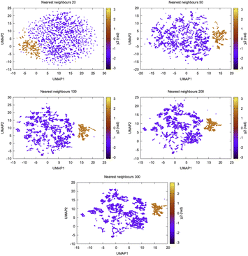
log2![[thin space (1/6-em)]](https://www.rsc.org/images/entities/char_2009.gif) pj|i. Perplexity can be thought as a measure of nearest neighbours and the choice of perplexity heavily determines the outcome of t-SNE (Fig. 10).
pj|i. Perplexity can be thought as a measure of nearest neighbours and the choice of perplexity heavily determines the outcome of t-SNE (Fig. 10).
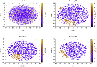 | ||
| Fig. 10 Projection of first two t-SNE components along χ2 angle of Tyr77 in plasmepsin-II shows how the embedding changes with perplexity. Further t-SNE performed on the high dimensional torsional features (Table 1 in ESI‡) didn't manage to separate flipping along χ2 which is a slow degree of freedom. It further shows that clustering on top of t-SNE reduced dimensions will generate artificial clusters which in reality belong to same metastable state. | ||
t-SNE aims to learn a low dimensional manifold  in such a way that the new conditional probability
  reflects similarity with pj|i.
  can be expressed as:
 | (21) |
The distance based metrics  is a heavily tailed distribution. In t-SNE, Student t-distribution has been used to measure the similarity between low-dimensional data-points so that the points that are far apart have
  which are invariant of perturbation. The algorithm aims to minimise the Kullback–Leibler divergence (other measures of similarity e.g. Jensen–Shannon divergence, Bhattacharya distance can be explored to improve the embedding result) by comparing joint probability distributions P′ (low-dimensional) and P (high-dimensional):
 | (22) |
The gradient descent algorithm is usually effective for small datasets but performs poorly in case of larger datasets. Recently a time-lagged version of t-SNE42 was proposed using inspiration from time-lagged ICA (TICA). However, the stochastic nature (mainly due to perplexity) of t-SNE (as shown in Fig. 10 and discussed in ref. 43) prevents its use as a meaningful CV for reconstructing trustworthy free energy surface and calculating kinetics from MD simulation. Clustering on the top of t-SNE embedding can also produce artificial clusters which might trick the user of thinking that it discovers new metastable states but in reality they belong to the same free energy basin.
Softwares: time-lagged version of t-SNE can be accessed here: https://github.com/spiwokv/tltsne. Popular machine learning package scikit-learn also has a t-SNE module: https://scikit-learn.org/stable/modules/generated/sklearn.manifold.TSNE.html. MODE-TASK https://github.com/RUBi-ZA/MODE-TASK a python toolkit for analysing MD simulation has an integrated t-SNE functionality. Tensorboard embedding projector https://projector.tensorflow.org has a graphical user interface to perform t-SNE.
In recent years, several other dimensionality reduction methods such as spectral gap optimization of order parameters (SGOOP),44 isomap45 (https://scikit-learn.org/stable/modules/generated/sklearn.manifold.Isomap.html), dynamic mode decomposition (DMD)46 (https://mathlab.github.io/PyDMD/, see ref. 47 for similarity between DMD and TICA and their variants), multi-dimensional scaling (MDS),45 UMAP48,49 (https://umap-learn.readthedocs.io/en/latest/, Fig. 11), iVIS50 (https://bering-ivis.readthedocs.io/en/latest/) which are similar to some of the aforementioned algorithms, were applied on temporal data from MD simulation. Further, sparse regression based dimensionality reduction method sparse identification of nonlinear dynamical systems (SINDy)51 can possibility be applied on temporal data from MD simulation to discover linear combinations of features which best captures conformational dynamics in macromolecules. Recent review by Glielmo et al.52 summarises mathematical concepts, strengths and limitations as well as applicability of few such methods in analysing high-dimensional data from MD simulations.
VAE takes high dimensional vector r = [r1,r2, …, rN]T as inputs. Each components of r are probability distributions along geometric or abstract CVs. The encoder part of the VAE encodes the high dimensional data into the latent variables z. The joint probability distribution of input and latent variables, p(r, z) can be expressed as:
| p(r,z) = p(r|z)p(z) | (23) |
The generative process can be expressed as:
(a) sampling latent variables, zi from the prior distribution p(z) and
(b) sampling of data point ri from the likelihood p(r|z) which is conditional on the latent variables z.
The goal of VAE is to infer good approximation of the latent variables (z) given input data (r) which is equivalent to calculate the posterior distribution p(z|r) as following:
 | (24) |
| p(r) = ∫p(r|z)p(z)dz | (25) |
Estimation of p(r) is a computationally expensive process as it requires integrating over all the possible values of z. VAE approximates the posterior distribution p(z|r) by a new distribution q(z|r) (tractable distribution). If qλ(z|r) is similar to p(z|r) then we can use it to approximate p(r). λ is the hyper-parameter which indicates type of distribution. If q(z|r) a Gaussian distribution then λri = (μri,σri2) where μ is the mean and σ2 is the variance of latent variables of each input component.
Now we want to measure how well qλ(z|r) approximates p(z|r). VAE uses Kullback–Leibler (KL) divergence to measure information loss between two probability densities as described below:
 | (26) |
We can reformulate eqn (26) as follows:
log![[thin space (1/6-em)]](https://www.rsc.org/images/entities/char_2009.gif) p(r) = ELBO(λ) + KL(qλ(z|r)‖p(z|r)) p(r) = ELBO(λ) + KL(qλ(z|r)‖p(z|r))
| (27) |
From eqn (27) we can see that minimising KL divergence (KL divergence is always greater or equal to zero) is equivalent to maximising Evidence Lower Bound (ELBO). It allows us to bypass the hard task of minimising KL divergence between the approximate q(z|r) and true posterior p(z|r), instead we maximise ELBO. ELBO term can be further expressed as follows:
 | (28) |
Eqn (28) is known the VAE loss function (L):
 | (29) |
In biomolecular simulation deep neural network (DNN) encodes input data and computes λ which approximates qw(z|r, λ). The decoder takes p(z) as input and maps into original distribution pw′(r|z). w and w′ acts as a neural network weights. w transforms the input data within the neural network hidden layers and the resulting latent variable is a combination of linear transformations that are modified by non-linear activation functions. Weights are learnable parameters during VAE training. The value of weight dictates the importance of a variable. A higher weight value corresponding an input component indicates that it will have a significant influence on the output.
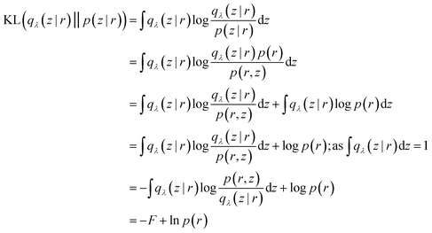
Mathematically speaking, the reason behind VAE's popularity in biomolecular simulation community is due to the interconnectivity between loss function and variational free energy (F):
 | (30) |
∫qλ(z|r)![[thin space (1/6-em)]](https://www.rsc.org/images/entities/char_2009.gif) log log![[thin space (1/6-em)]](https://www.rsc.org/images/entities/char_2009.gif) p(r)dz = 1 p(r)dz = 1
| (31) |
By comparing eqn (26) with (31) we can conclude that the variational free energy (F) is equal to the ELBO(λ). Thus minimising KL divergence is equivalent to maximising the variational free energy (F).
Fig. 12 shows a typical architecture of VAE in context of biomolecular simulation. The encoder part of the VAE acts as a non-linear dimensionality reduction of input r. Whereas the decoder DNN acts an input reconstruction. VAE has been primarily used a dimensionality reduction method to compress multi-variate probability distributions. The weights of the encoder layer which maps the input data onto the latent layer has been further used to drive enhanced sampling simulations such as metadynamics.55 As the latent layer of VAE represents a non-linear combination of input data hence it reduces the need of multiple CVs as inputs in metadynamics (traditionally metadynamics is limited to a maximum of two CVs). However in terms of exploration of the conformational space, metadynamics bias applied to multiple CVs using parallel-bias metadynamics framework will be equivalent to using VAE's latent variable as CV in a 1D metadynamics. Several different flavours of VAEs have been developed which mainly differs in their architecture (e.g. β-VAE which uses an additional hyper-parameter β to learn disentangled latent variables by controlling the KL divergence56) and types of inputs (e.g. VAE-SNE which takes output of tSNE as inputs, DMD-VAE which can take multiple dynamic modes as inputs, SINDy-VAE which takes outputs from SINDy algorithm as inputs). However, combining autoencoder based machine learning architecture with enhanced sampling algorithms or MD codes is a difficult task in practice. Recently, Chen and co-workers57 proposed a user-friendly tool called MLCV which uses an autoencoder architecture to transform arbitrarily defined CVs to autoencoder learned CVs and integrate it with MD engines for enhanced sampling calculations. In future, MLCV can be extended by adding different variants of VAE to capture conformational heterogeneity and drive enhanced sampling calculations.
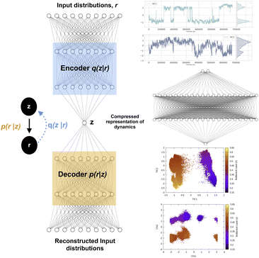 | ||
| Fig. 12 Left panel showing a typical architecture of deep neural network based variational autoencoder. The input distributions r can be probability distributions of geometric variables, TICs, DMD etc. Right panel shows how latent layer of variational autoencoder learned the dynamics of the system using TICs as inputs. TICs were generated using χ1 and χ2 angles of residues present in the flap region of plasmepsin-II (Table 1 in ESI‡) with lag-time 1000. Following hyper-parameters were used during the training process of VAE, no of hidden layers = 2, no of neurons in each hidden layer = 20, epochs = 100, batch size = 500, learning rate = 1e − 2. | ||
Softwares & implementations: VAEs for post-processing high-dimensional time-series data generated from MD simulation can be implemented using popular machine learning libraries e.g. PyTorch, Tensorflow, Keras etc. Recently Pande and co-workers58(variational dynamic encoder: https://github.com/msmbuilder/vde) as well as Tiwary and colleagues59 (RAVE: https://github.com/tiwarylab/RAVE) applied VAE to compress high-dimensional temporal data and able to capture non-linear dynamics in context of protein folding, protein-ligand binding/unbinding etc. A collection of prebuilt VAE architectures implemented with PyTorch (https://github.com/AntixK/PyTorch-VAE) opens up the possibility to evaluate VAE variants in context of MD simulation.
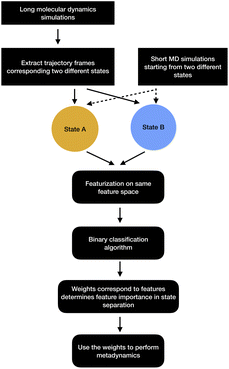 | ||
| Fig. 13 Schematic representation of showing how binary classifiers can be used to separate metastable states and drive enhanced sampling calculations. | ||
2.2.7.1 Support vector machine. Let A and B are two metastable states which can be represented by unique points in space where each point belongs to high-dimensional feature vector r = [r1, …, rN]. The goal of SVM algorithm is to find a separating hyperplane that maximises the minimum distance between closest points (support vectors) of the two metastable states (otherwise known as classes):
 | (32) |
 is the normalisation term. The SVM algorithm then maximise the minimum distance w* = argw max[minndH]. In context of biomolecular simulation, eqn (32) acts a CV which can separate metastable states and drive enhanced sampling simulations (Fig. 14). Sultan and Pande showed how dH can be used as CV within metadynamics framework to sample conformational space of alanine dipeptide and chignolin folding.61 SVM algorithm can be further extended for non-linear classification by using kernel trick as explained before.
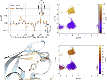 | ||
| Fig. 14 Coefficients (weights) correspond to linear SVM and passive aggressive classifier63 trained on χ1 and χ2 angles of residue 74–84 (Table 1 in ESI‡) in plasmepsin-II showing the importance of sin χ2 (feature 21) and cos χ2 (feature 25) in separating two metastable basins, normal (χ2 ∼ − 1 rad) and flipped (χ2 ∼ 2 rad). 50 ns trajectories from each basins were used for training purpose using the scheme described in Fig. 13. Further χ1 and χ2 angles of Tyr77 projected along classifier decision boundaries demonstrated separation of metastable states. Snapshots corresponding normal (grey) and flipped (blue) states are also highlighted. | ||
2.2.7.2 Linear discriminant analysis. Linear discriminant analysis (LDA) is a supervised dimensionality reduction method which finds linear combinations of features that best separates two or more metastable states.64 Imagine two metastable states with common features
![[r with combining right harpoon above (vector)]](https://www.rsc.org/images/entities/i_char_0072_20d1.gif) have means
have means ![[small mu, Greek, vector]](https://www.rsc.org/images/entities/i_char_e0e9.gif) A and
A and ![[small mu, Greek, vector]](https://www.rsc.org/images/entities/i_char_e0e9.gif) B and covariances ΣA and ΣB. The linear combinations of features
B and covariances ΣA and ΣB. The linear combinations of features ![[w with combining right harpoon above (vector)]](https://www.rsc.org/images/entities/i_char_0077_20d1.gif) ·
·![[r with combining right harpoon above (vector)]](https://www.rsc.org/images/entities/i_char_0072_20d1.gif) (
(![[w with combining right harpoon above (vector)]](https://www.rsc.org/images/entities/i_char_0077_20d1.gif) is known as LDA coefficients) will have means
is known as LDA coefficients) will have means ![[w with combining right harpoon above (vector)]](https://www.rsc.org/images/entities/i_char_0077_20d1.gif) ·
·![[small mu, Greek, vector]](https://www.rsc.org/images/entities/i_char_e0e9.gif) A,B and variances
A,B and variances ![[w with combining right harpoon above (vector)]](https://www.rsc.org/images/entities/i_char_0077_20d1.gif) TΣA,B
TΣA,B![[w with combining right harpoon above (vector)]](https://www.rsc.org/images/entities/i_char_0077_20d1.gif) . LDA objective function separates two distributions by taking ratio between variance between the classes to variance within classes:
. LDA objective function separates two distributions by taking ratio between variance between the classes to variance within classes:
 | (33) |
Mathematically it can shown that the maximum separation occurs when  . LDA algorithm can be generalised to more than one classes (Multi-class LDA). Eqn (33) acts as a CV in metadynamics to drive transition between state A and B. Recently Parrinello and co-workers used a harmonic version of LDA (HLDA) as a CV to study folding of a small protein and protein-ligand binding/unbinding.62,65 The framework of LDA can be patched with neural network (Deep-LDA) as well as kernel trick in order to introduce non-linearity. Recently Deep-LDA framework has been applied in SAMPL5 host–guest systems to accurately calculate binding free energy and to understand the role of water molecule in ligand binding.66
In order to apply classifier algorithms to separate metastable states one first need to sample different metastable states. However, sampling of metastable states separated by high entropic barrier often requires ultra-long MD simulations or enhanced sampling simulations e.g. parallel-tempering. Further, one needs to carefully choose a set of features that can separate a set of metastable states. For complex systems, selection of such features are not trivial and often needs significant amount of trial and error.
Softwares: scikit-learn's supervised learning module incorporates both LDA and SVM algorithms for training purpose. It further integrates various other supervised learning algorithms that can be applied to classify metastable states and act as CVs in enhanced sampling simulations.
Softwares: Tiwary and co-workers67 used LSTM based neural network to predict temporal evolution in model systems. Their code can be accessed here: https://github.com/tiwarylab/LSTM-predict-MD.Tensorflow (https://www.tensorflow.org/text/tutorials/transformer and https://www.tensorflow.org/guide/keras/rnn) and Pytorch (https://github.com/jdb78/pytorch-forecasting) based time-series forecasting modules can be used for this purpose. Zeng and co-workers68 used LSTM/transformers to predict temporal evolution of different CVs in alanine dipeptide (https://github.com/Wendysigh/LSTM-Transformer-for-MD).
3 Use of machine learning/AI in CV selection: the hype
Recently numerous papers reported different combinations of abstract order parameters to capture conformational dynamics and molecular recognition of macromolecules. In one such case neural network based LDA (Deep-LDA) approach has been applied on SAMPL5 host–guest systems to estimate binding free energy.66 Previously funnel metadynamics using simple distance CV combined with artificial restraint along binding-site solvation managed to accurately predict the binding free energy for the same host–guest systems.70 We can ask a question: was deep-LDA framework necessary for a relatively simple problem such as host–guest binding/unbinding which was previously solved using simple geometric CVs? One can argue that deep-LDA framework is more natural as it didn't impose any artificial restraint along solvent degrees of freedom. In SAMPL5 host–guest systems, the solvation (when the binding site is occupied by long-lived water molecule) of the binding site is a slow process (Fig. S2 in ref. 70). In principal TICA/SGOOP (which by design capable of capturing slow degrees of freedom) could have solved such a problem. Further, deep-LDA method is a slightly fancier application of previously described work which uses binary classifiers as CVs to drive conformational sampling.61 This is a classic example where the developers of a CV discovery method used buzzwords to solve a trivial problem without pointing out how exactly such deep learning based CV is superior compared to other geometric or abstract order parameters.In another case authors used TICs/SGOOPs as inputs within a VAE and used the VAE's latent layer as CV for enhanced sampling.55,71 Such an approach is advantageous if an enhanced sampling algorithm is limited to driving along one CV. Further, the eigenvalues corresponding each TIC/SGOOP can be used to filter geometric CVs which then can be used as an input in VAE. This approach can be seen as an extension of previous approach where one inputs TICs/SGOOPs directly into VAE. However a critic can ask: is there any advantage in terms of sampling if one uses VAE's latent layer vs. multiple CVs (using parallel-bias metadynamics) within metadynamics (Fig. 16) and more importantly can you call such method artificial intelligence (AI)?
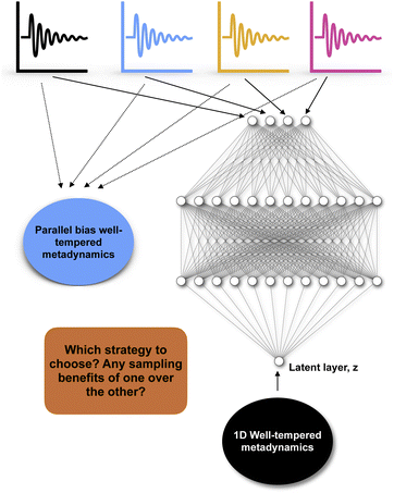 | ||
| Fig. 16 Describes dilemma of choosing an enhanced sampling strategy over other: in case of four different CVs (depicted by black, blue, yellow and magenta) one can either choose to perform a parallel-bias72 variant of well-tempered metadynamics simulation or feed these four CVs within variational autoencoder and uses the latent layer of variational autoencoder as CV in 1D well-tempered metadynamics. | ||
Most of the algorithms described in the previous section either require extensive sampling or prior knowledge about metastable states in order to capture conformational changes in biomolecules. These algorithms can be best described as data driven machine learning algorithms which solves a deterministic closed set finite problems using large amount of training data.
In case of complex biological process e.g. protein-ligand unbinding, protein–protein binding, protein folding involving multiple metastable states and lack of prior knowledge about transition states, an iterative machine learning based CV discovery method combined with enhanced sampling can accelerate sampling of the underlying free energy surface.73,74 However such protocol also requires initial guess of CVs. An near-term artificial general intelligence (AGI) on other hand will learn about the dynamical system on the fly without the external supervision (e.g. feature selection, choice of algorithms, tuning of hyper-parameters etc) and extract observables that can be confirmed by biophysical experiments. Development of such self-aware AGI will require significant innovation in terms of novel algorithms and software design. Until that time, the biomolecular simulation community should refrain from using the word AI in context of identifying low-dimensional representation to approximate kinetics and thermodynamics of biomolecular systems.
4 Conclusions
In recent years data-driven machine learning models impacted the field of biomolecular simulation and have been applied in context of protein folding, protein-ligand/protein binding and capturing rare conformational changes during molecular simulation. However a real challenge in comparing the power of different machine learning models is due to absence of a common dataset. We believe that the basic pancreatic trypsin inhibitor (BPTI) can act as a reasonable dataset to test different algorithms. The reasons behind that are accessibility of (a) 1 ms long MD simulation and (b) experimental observables such as NMR order parameter, kinetics of ring flipping (rare events) and protection factors (measure of amide hydrogen–deuterium exchange). Further transient loop opening of BPTI which leads to amide hydrogen–deuterium exchange29 and aromatic ring flipping75,76 are the rare events that can be captured by both simulation and experiments. Transient loop opening leads to amide hydrogen–deuterium exchange which is represented by a metric called protection factor. A good machine learning model for CV discovery combined with an enhanced sampling framework should sample the rare events and predict experimental observables (rate of ring flipping and protection factors). Recent metadynamics based investigation with geometric CVs (dihedral angles) highlighted the challenge of sampling slow ring flipping in BPTI. In order to live up to the hype, machine learning based abstract CVs should do better in sampling such rare events and predict kinetics.A major leap forward in combining machine learning with MD will be prediction of multi-dimensional spatiotemporal evolution of biomolecular dynamics. Recently, transformer network has been applied to model crowd motion dynamics which managed to achieve state-of-the-art performance on commonly used pedestrian prediction datasets.77 In future extension of such work can be applied in context of MD simulation to predict temporal evolution of CVs and corresponding spatial representation. However prediction of spatiotemporal evolution of bimolecular structure without correctly capturing the water dynamics doesn't model physical reality as water plays integral role in molecular recognition and conformational dynamics of biomolecules. We hope breakthroughs in quantum computer together with novel machine learning algorithms will make spatiotemporal prediction of solvated biomolecular system a reality, until then we have to carefully select geometric/abstract CVs to capture dynamics of biomolecules from atomistic simulations.
Author contributions
SB conceived the idea, performed all the calculations and wrote the manuscript.Conflicts of interest
There are no conflicts to declare.Acknowledgements
The computations were performed on computer resources provided by the Swedish National Infrastructure for Computing (SNIC) at LUNARC (Lund University) and HPC2N (Umeå University). The author thanks Borna Novak for carefully reading the manuscript.Notes and references
- S. A. Hollingsworth and R. O. Dror, Neuron, 2018, 99, 1129–1143 CrossRef CAS PubMed.
- J. Fan and J. Lv, Stat. Sin., 2010, 20, 101–148 Search PubMed.
- S. Bhakat, RSC Adv., 2021, 11, 11026–11047 RSC.
- S. Bhakat and P. Söderhjelm, J. Chem. Inf. Model., 2022, 62, 914–926 CrossRef CAS PubMed.
- G. Bussi and A. Laio, Nat. Rev. Phys., 2020, 2, 200–212 CrossRef.
- Y. Wang, J. M. Lamim Ribeiro and P. Tiwary, Curr. Opin. Struct. Biol., 2020, 61, 139–145 CrossRef CAS PubMed.
- M. Chen, Eur. Phys. J. B, 2021, 94, 211 CrossRef CAS PubMed.
- O. Valsson, P. Tiwary and M. Parrinello, Annu. Rev. Phys. Chem., 2016, 67, 159–184 CrossRef CAS PubMed.
- J. S. Patel, A. Berteotti, S. Ronsisvalle, W. Rocchia and A. Cavalli, J. Chem. Inf. Model., 2014, 54, 470–480 CrossRef CAS PubMed.
- W. You, Z. Tang and C.-e. A. Chang, J. Chem. Theory Comput., 2019, 15, 2433–2443 CrossRef CAS PubMed.
- L. S. Dodda, J. Tirado-Rives and W. L. Jorgensen, J. Phys. Chem. B, 2019, 123, 1741–1748 CrossRef CAS PubMed.
- F. Sittel and G. Stock, J. Chem. Phys., 2018, 149, 150901 CrossRef PubMed.
- F. Persson and B. Halle, J. Am. Chem. Soc., 2013, 135, 8735–8748 CrossRef CAS PubMed.
- D. E Shaw, P. Maragakis, K. Lindorff-Larsen, S. Piana, R. O. Dror, M.P. Eastwood, J.A. Bank, J.M. Jumper, J.K. Salmon, Y. Shan and W. Wriggers, Science, 2010, 330, 341–346 CrossRef CAS PubMed.
- G. A. Tribello, M. Bonomi, D. Branduardi, C. Camilloni and G. Bussi, Comput. Phys. Commun., 2014, 185, 604–613 CrossRef CAS.
- D. R. Roe and T. E. Cheatham, J. Chem. Theory Comput., 2013, 9, 3084–3095 CrossRef CAS PubMed.
- N. Michaud-Agrawal, E. J. Denning, T. B. Woolf and O. Beckstein, J. Comput. Chem., 2011, 32, 2319–2327 CrossRef CAS PubMed.
- R. T. McGibbon, K. A. Beauchamp, M. P. Harrigan, C. Klein, J. M. Swails, C. X. Hernández, C. R. Schwantes, L.-P. Wang, T. J. Lane and V. S. Pande, Biophys. J., 2015, 109, 1528–1532 CrossRef CAS PubMed.
- F. Sittel, T. Filk and G. Stock, J. Chem. Phys., 2017, 147, 244101 CrossRef PubMed.
- M. P. Harrigan, M. M. Sultan, C. X. Hernández, B. E. Husic, P. Eastman, C. R. Schwantes, K. A. Beauchamp, R. T. McGibbon and V. S. Pande, Biophys. J., 2017, 112, 10–15 CrossRef CAS PubMed.
- M. K. Scherer, B. Trendelkamp-Schroer, F. Paul, G. Pérez-Hernández, M. Hoffmann, N. Plattner, C. Wehmeyer, J.-H. Prinz and F. Noé, J. Chem. Theory Comput., 2015, 11, 5525–5542 CrossRef CAS PubMed.
- L. Molgedey and H. G. Schuster, Phys. Rev. Lett., 1994, 72, 3634–3637 CrossRef PubMed.
- G. Pérez-Hernández, F. Paul, T. Giorgino, G. De Fabritiis and F. Noé, J. Chem. Phys., 2013, 139, 015102 CrossRef PubMed.
- C. R. Schwantes and V. S. Pande, J. Chem. Theory Comput., 2013, 9, 2000–2009 CrossRef CAS PubMed.
- M. M. Sultan and V. S. Pande, J. Chem. Theory Comput., 2017, 13, 2440–2447 CrossRef PubMed.
- S. Schultze and H. Grubmüller, J. Chem. Theory Comput., 2021, 17, 5766–5776 CrossRef CAS PubMed.
- T. Blaschke, P. Berkes and L. Wiskott, Neural Comput., 2006, 18, 2495–2508 CrossRef PubMed.
- T. Blaschke and L. Wiskott, Independent Component Analysis and Blind Signal Separation, Berlin, Heidelberg, 2004, pp. 742–749 Search PubMed.
- F. Persson and B. Halle, Proc. Natl. Acad. Sci. U. S. A., 2015, 112, 10383–10388 CrossRef CAS PubMed.
- M. Hoffmann, M. Scherer, T. Hempel, A. Mardt, B. de Silva, B. E. Husic, S. Klus, H. Wu, N. Kutz, S. L. Brunton and F. Noé, Mach. learn.: sci. technol., 2021, 3, 015009 Search PubMed.
- C. R. Schwantes and V. S. Pande, J. Chem. Theory Comput., 2015, 11, 600–608 CrossRef CAS PubMed.
- M. P. Harrigan and V. S. Pande, bioRxiv, 2017 DOI:10.1101/123752.
- C. Ross, B. Nizami, M. Glenister, O. Sheik Amamuddy, A. R. Atilgan, C. Atilgan and Ö. T. Bishop, Bioinformatics, 2018, 34, 3759–3763 CrossRef CAS PubMed.
- F. Noé and C. Clementi, J. Chem. Theory Comput., 2015, 11, 5002–5011 CrossRef PubMed.
- B. Nadler, S. Lafon, I. Kevrekidis and R. Coifman, Advances in Neural Information Processing Systems, 2006 Search PubMed.
- W. Zheng, M. A. Rohrdanz and C. Clementi, J. Phys. Chem. B, 2013, 117, 12769–12776 CrossRef CAS PubMed.
- A. L. Ferguson, A. Z. Panagiotopoulos, P. G. Debenedetti and I. G. Kevrekidis, Proc. Natl. Acad. Sci. U. S. A., 2010, 107, 13597–13602 CrossRef CAS PubMed.
- A. L. Ferguson, A. Z. Panagiotopoulos, I. G. Kevrekidis and P. G. Debenedetti, Chem. Phys. Lett., 2011, 509, 1–11 CrossRef CAS.
- S.-T. Tsai, Z. Smith and P. Tiwary, J. Chem. Theory Comput., 2021, 17, 6757–6765 CrossRef CAS PubMed.
- L. van der Maaten and G. Hinton, J. Mach. Learn. Res., 2008, 9, 2579–2605 Search PubMed.
- M. Wattenberg, F. Viégas and I. Johnson, Distill, 2016 DOI:10.23915/distill.00002.
- V. Spiwok and P. Kříž, Front. Mol. Biosci., 2020, 7, 132 CrossRef CAS PubMed.
- T. Chari, J. Banerjee and L. Pachter, bioRxiv, 2021 DOI:10.1101/2021.08.25.457696.
- P. Tiwary and B. J. Berne, Proc. Natl. Acad. Sci. U. S. A., 2016, 113, 2839–2844 CrossRef CAS PubMed.
- B. Ghojogh, A. Ghodsi, F. Karray and M. Crowley, Multidimensional Scaling, Sammon Mapping, and Isomap: Tutorial and Survey, 2020 Search PubMed.
- J. H. Tu, C. W. Rowley, D. M. Luchtenburg, S. L. Brunton and J. N. Kutz, J. Comput. Dyn., 2014, 1, 391–421 Search PubMed.
- S. Klus, F. Nüske, P. Koltai, H. Wu, I. Kevrekidis, C. Schütte and F. Noé, J. Nonlinear Sci., 2018, 28, 985–1010 CrossRef.
- L. McInnes, J. Healy and J. Melville, UMAP: Uniform Manifold Approximation and Projection for Dimension Reduction, 2020 Search PubMed.
- F. Trozzi, X. Wang and P. Tao, J. Phys. Chem. B, 2021, 125, 5022–5034 CrossRef CAS PubMed.
- H. Tian and P. Tao, J. Chem. Inf. Model., 2020, 60, 4569–4581 CrossRef CAS PubMed.
- S. L. Brunton, J. L. Proctor and J. N. Kutz, Proc. Natl. Acad. Sci. U. S. A., 2016, 113, 3932–3937 CrossRef CAS PubMed.
- A. Glielmo, B. E. Husic, A. Rodriguez, C. Clementi, F. Noé and A. Laio, Chem. Rev., 2021, 121, 9722–9758 CrossRef CAS PubMed.
- D. P. Kingma and M. Welling, Found. Trends Mach. Learn., 2019, 12, 307–392 CrossRef.
- D. P. Kingma and M. Welling, Auto-Encoding Variational Bayes, 2014 Search PubMed.
- M. M. Sultan, H. K. Wayment-Steele and V. S. Pande, J. Chem. Theory Comput., 2018, 14, 1887–1894 CrossRef CAS PubMed.
- C. P. Burgess, I. Higgins, A. Pal, L. Matthey, N. Watters, G. Desjardins and A. Lerchner, Understanding disentangling in β-VAE, 2018 Search PubMed.
- H. Chen, H. Liu, H. Feng, H. Fu, W. Cai, X. Shao and C. Chipot, J. Chem. Inf. Model., 2022, 62, 1–8 CrossRef CAS PubMed.
- C. X. Hernández, H. K. Wayment-Steele, M. M. Sultan, B. E. Husic and V. S. Pande, Phys. Rev. E, 2018, 97, 062412 CrossRef PubMed.
- J. M. L. Ribeiro, P. Bravo, Y. Wang and P. Tiwary, J. Chem. Phys., 2018, 149, 072301 CrossRef PubMed.
- N. Mohanty, A. L.-S. John, R. Manmatha and T. Rath, Handbook of Statistics, Elsevier, 2013, vol 31, pp. 249–267 Search PubMed.
- M. M. Sultan and V. S. Pande, J. Chem. Phys., 2018, 149, 094106 CrossRef PubMed.
- D. Mendels, G. Piccini, Z. F. Brotzakis, Y. I. Yang and M. Parrinello, J. Chem. Phys., 2018, 149, 194113 CrossRef PubMed.
- K. Crammer, O. Dekel, J. Keshet, S. Shalev-Shwartz and Y. Singer, J. Mach. Learn. Res., 2006, 7, 551–585 Search PubMed.
- R. A. Fisher, Ann. Hum. Genet., 1936, 7, 179–188 Search PubMed.
- R. Capelli, A. Bochicchio, G. Piccini, R. Casasnovas, P. Carloni and M. Parrinello, J. Chem. Theory Comput., 2019, 15, 3354–3361 CrossRef CAS PubMed.
- V. Rizzi, L. Bonati, N. Ansari and M. Parrinello, Nat. Commun., 2021, 12, 93 CrossRef CAS PubMed.
- S.-T. Tsai, E.-J. Kuo and P. Tiwary, Nat. Commun., 2020, 11, 5115 CrossRef CAS PubMed.
- W. Zeng, S. Cao, X. Huang and Y. Yao, A Note on Learning Rare Events in Molecular Dynamics using LSTM and Transformer, 2021 Search PubMed.
- B. Lim and S. Zohren, Philos. Trans. R. Soc., A, 2021, 379, 20200209 CrossRef PubMed.
- S. Bhakat and P. Söderhjelm, J. Comput.-Aided Mol. Des., 2017, 31, 119–132 CrossRef CAS PubMed.
- S. Pant, Z. Smith, Y. Wang, E. Tajkhorshid and P. Tiwary, J. Chem. Phys., 2020, 153, 234118 CrossRef CAS PubMed.
- J. Pfaendtner and M. Bonomi, J. Chem. Theory Comput., 2015, 11, 5062–5067 CrossRef CAS PubMed.
- S. Pant, Z. Smith, Y. Wang, E. Tajkhorshid and P. Tiwary, J. Chem. Phys., 2020, 153, 234118 CrossRef CAS PubMed.
- J. M. Lamim Ribeiro and P. Tiwary, J. Chem. Theory Comput., 2019, 15, 708–719 CrossRef CAS PubMed.
- U. Weininger, K. Modig and M. Akke, Biochemistry, 2014, 53, 4519–4525 CrossRef CAS PubMed.
- M. Kulkarni and P. Söderhjelm, bioRxiv, 2021 DOI:10.1101/2021.01.07.425261.
- C. Yu, X. Ma, J. Ren, H. Zhao and S. Yi, Spatio-Temporal Graph Transformer Networks for Pedestrian Trajectory Prediction, 2020 Search PubMed.
Footnotes |
| † Major part of the article was written when the author was affiliated to Division of Biophysical Chemistry, Center for Molecular Protein Science, Department of Chemistry, Lund University, Sweden and Department of Biochemistry and Molecular Biophysics, Washington University School of Medicine, St Louis, Missouri, USA. |
| ‡ Electronic supplementary information (ESI) available. See https://doi.org/10.1039/d2ra03660f |
| This journal is © The Royal Society of Chemistry 2022 |

