
 Open Access Article
 This Open Access Article is licensed under a Creative Commons Attribution-Non Commercial 3.0 Unported Licence
BonDNet: a graph neural network for the prediction of bond dissociation energies for charged molecules†
Mingjian
Wen
 ab,
Samuel M.
Blau
b,
Evan Walter Clark
Spotte-Smith
ab,
Shyam
Dwaraknath
b and
Kristin A.
Persson
*ac
ab,
Samuel M.
Blau
b,
Evan Walter Clark
Spotte-Smith
ab,
Shyam
Dwaraknath
b and
Kristin A.
Persson
*ac
aDepartment of Materials Science and Engineering, University of California, Berkeley, CA 94720, USA
bEnergy Technologies Area, Lawrence Berkeley National Laboratory, Berkeley, CA 94720, USA
cMolecular Foundry, Lawrence Berkeley National Laboratory, Berkeley, CA 94720, USA. E-mail: kapersson@lbl.gov
First published on 8th December 2020
Abstract
A broad collection of technologies, including e.g. drug metabolism, biofuel combustion, photochemical decontamination of water, and interfacial passivation in energy production/storage systems rely on chemical processes that involve bond-breaking molecular reactions. In this context, a fundamental thermodynamic property of interest is the bond dissociation energy (BDE) which measures the strength of a chemical bond. Fast and accurate prediction of BDEs for arbitrary molecules would lay the groundwork for data-driven projections of complex reaction cascades and hence a deeper understanding of these critical chemical processes and, ultimately, how to reverse design them. In this paper, we propose a chemically inspired graph neural network machine learning model, BonDNet, for the rapid and accurate prediction of BDEs. BonDNet maps the difference between the molecular representations of the reactants and products to the reaction BDE. Because of the use of this difference representation and the introduction of global features, including molecular charge, it is the first machine learning model capable of predicting both homolytic and heterolytic BDEs for molecules of any charge. To test the model, we have constructed a dataset of both homolytic and heterolytic BDEs for neutral and charged (−1 and +1) molecules. BonDNet achieves a mean absolute error (MAE) of 0.022 eV for unseen test data, significantly below chemical accuracy (0.043 eV). Besides the ability to handle complex bond dissociation reactions that no previous model could consider, BonDNet distinguishes itself even in only predicting homolytic BDEs for neutral molecules; it achieves an MAE of 0.020 eV on the PubChem BDE dataset, a 20% improvement over the previous best performing model. We gain additional insight into the model's predictions by analyzing the patterns in the features representing the molecules and the bond dissociation reactions, which are qualitatively consistent with chemical rules and intuition. BonDNet is just one application of our general approach to representing and learning chemical reactivity, and it could be easily extended to the prediction of other reaction properties in the future.
1 Introduction
The strength of chemical bonds is one of the fundamental and decisive elements in determining the reactivity and selectivity of molecules undergoing chemical reactions.1–3 The bond dissociation energy (BDE), the amount of energy needed to break a bond in a molecule, is one measure of chemical bond strength. BDEs play a significant role in many chemical applications. BDE analysis is a typical key first step in understanding chemical processes such as retrosynthesis,4–6 drug metabolism,3,7 biofuel combustion,8,9 photochemical decontamination of water pollutants,10 formation of side products in batteries and solar cells,11 and many others. Despite being a thermodynamic property, BDEs are also commonly applied to predict kinetic properties of reactions. For example, the Bell–Evans–Polanyi principle12,13 provides an efficient way to calculate the activation energies of reactions within a distinct family from BDE values; these activation energies can then be used with the Arrhenius equation14 to calculate the reaction rates.A bond dissociation reaction can be categorized into one of two types: homolysis
| A:B → A⋅ + B⋅ | (1) |
| A:B → [A:]− + [B]+ | (2) |
| [A:B]− → A⋅ + [B⋅]− | (3) |
is the counterpart of eqn (1) for a −1 charged molecule. Whatever the bond dissociation type and the molecular charges are, the BDE is calculated as the energy change between the products and the reactant, ΔE = E(A) + E(B) − E(AB). Historically, reaction enthalpy has been used, as these values have been tabulated in textbooks;15,16 recently, however, the Gibbs free energy has become prevalent in the chemical literature.17–20 Quantum mechanical computational chemistry methods like density functional theory (DFT) are well suited to calculate a large (∼103 to 104) but still limited number of BDEs with high accuracy.21,22 However, they become too computationally demanding to be widely adopted for chemical design of real-system reaction cascades,23 where millions of BDEs need to be calculated to screen for appropriate molecules or reactions. Machine learning models could be a promising alternative to provide orders of magnitude faster predictions without a significant sacrifice in accuracy. Contemporary machine learning methods, especially deep learning, have already demonstrated success in solving many chemistry problems, such as retrosynthesis planning,4–6,24 reaction products prediction,25–28 molecule generation,29–32 and molecular property prediction.33,34 The most crucial component of chemical machine learning models is a suitable molecular representation to extract information relevant to the problem of interest. Conventional approaches utilize feature engineering to encode variable-size molecules as fixed-length vectors that emphasize particular aspects of molecules deemed important for a property while ignoring others.35–38 However, these manually crafted molecular representations are not easily transferable to new problems. More recently, molecular representations have been automatically generated using graph neutral network (GNN) methods.39–43 GNNs treat molecules as graphs and learn molecular representations from data via message passing between atoms and bonds. Models based on GNNs can significantly outperform conventional methods that rely on manual feature engineering.44–46
For the prediction of BDEs, there already are several machine learning models relying on molecular representations either from manual feature engineering or GNNs. Early works restricted themselves to extremely small datasets of one or two bond types and trained simple learning algorithms such as polynomial fitting47 and support vector machines48 on manually crafted features. More recent works have leveraged high-throughout DFT calculations to generate larger BDE datasets of various bond types and have adopted neural networks as the learning algorithm. Qu et al.2 trained an associative neural network (ANN) on ∼12![[thin space (1/6-em)]](https://www.rsc.org/images/entities/char_2009.gif) 000 BDEs for molecules made up of C, H, O, N, and S atoms, achieving a mean absolute error (MAE) of 0.145 eV. St. John et al.3 trained ALFABET (a GNN model) on ∼290000 BDEs for molecules made up of C, H, O, and N atoms, achieving an MAE of 0.025 eV.3 These MAEs are close to or even below the chemical accuracy of 0.043 eV (i.e. 1 kcal mol−1).49 Despite their successes, current machine learning models for BDE prediction still suffer from two interdependent limitations. First, these models assume particular states of the products (e.g. neutral charge) and predict BDEs from the reactants by specifying the breaking bonds, without considering feature updates of the products. Second, these models are only applicable to the homolysis of neutral molecules as in eqn (1); heterolysis (eqn (2)) and bond dissociation of charged molecules (eqn (3)) are beyond their capabilities. This is likely due to the lack of publicly accessible BDE datasets for charged molecules or heterolytic bond dissociation. Unlike the homolysis of neutral molecules (eqn (1)) where the two products exhibit the same charge, cleaving a neutral molecule heterolytically (eqn (2)) or a charged molecule homolytically (eqn (3)) will yield products of different charges. Depending on which product possesses which charge, there might be several different possible ways for the bond to break, and thus several different values for the BDE. Without explicitly including product information, it is impossible for a model to distinguish between these different possible reactions.
000 BDEs for molecules made up of C, H, O, N, and S atoms, achieving a mean absolute error (MAE) of 0.145 eV. St. John et al.3 trained ALFABET (a GNN model) on ∼290000 BDEs for molecules made up of C, H, O, and N atoms, achieving an MAE of 0.025 eV.3 These MAEs are close to or even below the chemical accuracy of 0.043 eV (i.e. 1 kcal mol−1).49 Despite their successes, current machine learning models for BDE prediction still suffer from two interdependent limitations. First, these models assume particular states of the products (e.g. neutral charge) and predict BDEs from the reactants by specifying the breaking bonds, without considering feature updates of the products. Second, these models are only applicable to the homolysis of neutral molecules as in eqn (1); heterolysis (eqn (2)) and bond dissociation of charged molecules (eqn (3)) are beyond their capabilities. This is likely due to the lack of publicly accessible BDE datasets for charged molecules or heterolytic bond dissociation. Unlike the homolysis of neutral molecules (eqn (1)) where the two products exhibit the same charge, cleaving a neutral molecule heterolytically (eqn (2)) or a charged molecule homolytically (eqn (3)) will yield products of different charges. Depending on which product possesses which charge, there might be several different possible ways for the bond to break, and thus several different values for the BDE. Without explicitly including product information, it is impossible for a model to distinguish between these different possible reactions.
In this paper, we overcome these limitations and propose a general GNN model, Bond Dissociation Network (BonDNet), capable of predicting both homolytic and heterolytic BDEs for molecules of any charge. In addition to the atom and bond features widely used in previous GNNs for molecules,39–43 BonDNet adds global features50,51 to encode molecule-level information. Specifically, the total charge of a molecule is included as a global feature to distinguish molecules with the same connectivity but different charge. BonDNet then takes the differences of the atom, bond, and global features between the products and the reactant to represent a bond dissociation reaction.52–54 We show that these chemically inspired difference features assist the model in learning better representations of bond dissociation reactions, and thus, even when only predicting homolytic BDEs of neutral molecules, BonDNet surpasses previous models by a considerable margin. We trained BonDNet on a novel dataset consisting of both homolytic and heterolytic BDEs for neutral and charged (−1, and +1) molecules. The model achieves an MAE of 0.022 eV for unseen BDEs in this complex dataset, approaching the accuracy of the DFT method used to generate the data. Finally, we demonstrate how chemical insight can be extracted from BonDNet by analyzing the features representing the molecules and the reactions. An interface to use the developed model for the prediction of BDEs is provided via binder55 and can be accessed at https://github.com/mjwen/bondnet.
2 Methods
In molecular GNNs, molecules are represented as graphs, with atoms represented by nodes and chemical bonds represented by edges. Following ref. 50 and 51, we extend this representation by adding global features to encode molecule-level information and then denote a molecular graph as G = (E,V,u). In this molecular graph, E = {(ek,rk,sk)}k=1:Ne is the set of bonds (edges), where Ne is the total number of bonds in the molecule, and (ek,rk,sk) holds the information of the kth bond: ek is a vector of bond features (e.g. whether a bond is in a ring), and rk and sk are the indices of the two atoms forming the bond. Similarly, V = {vi}i=1:Nv is the set of atoms (nodes), where Nv is the total number of atoms in the molecule, and vi is a vector of features for atom i (e.g. atom type). Finally, u is a global feature vector of molecule-level information such as the total molecular charge.BonDNet has two major components. The first is a graph-to-graph (g2g) module that takes a molecular graph as input and yields the same molecular graph but with updated atom, bond, and global features. The g2g module is applied multiple times to learn better molecular representations from the data. The second component is a graph-to-property (g2p) module. Taking as input the molecular representations learned by the g2g module, the g2p module constructs chemically inspired representations of reactions and maps them to chemical properties (in this work, BDEs). In this section, we first provide a thorough discussion of the two components and then briefly introduce the input features and how the model is trained.
2.1 Graph-to-graph module
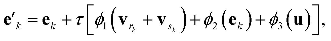
The g2g module takes a molecular graph G(E,V,u) as input, updates the bond, atom, and global features, and outputs the same molecular graph with updated features G(E′,V′,u′). The feature update scheme is based on the gated graph convolutional network (GatedGCN),56 which has been shown to consistently perform well for a number of regression and classification tasks across various datasets.57 The GatedGCN, however, can only operate on graphs having node and edge features. To support our molecular graph, we extend GatedGCN for graphs that also have global features.A schematic illustration of the g2g module of BonDNet is shown in Fig. 1a. First, each bond feature vector ek is updated from the feature vectors for the two atoms participating in the bond, vrk and vsk, the global feature vector u, and the current bond feature vector:
 | (4) |
 that form bonds with the atom, the formed bonds, and the global state:
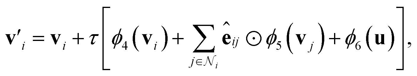 | (5) |
 | (6) |
 is another way to denote the bond feature
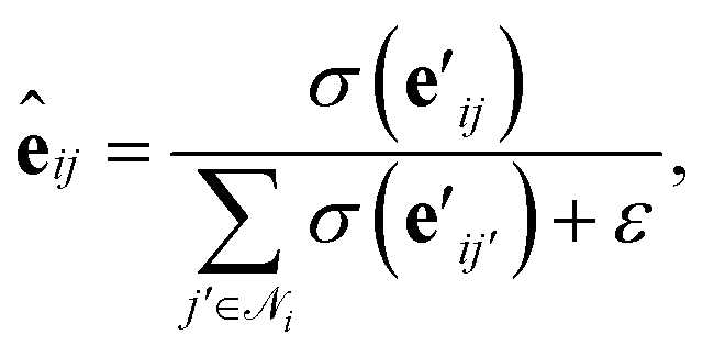
  such that atoms i and j form bond k, i.e. i = rk and j = sk. The edge gate
  can be regarded as a soft attention mechanism57 that enables neighboring atoms to contribute with different magnitude to the atom feature update. Finally, the global feature vector u is updated based on all atoms, all bonds, and itself:
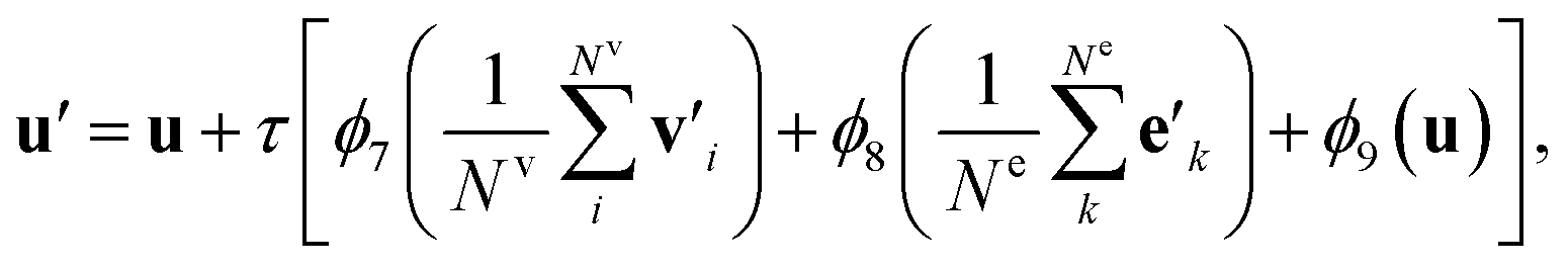 | (7) |
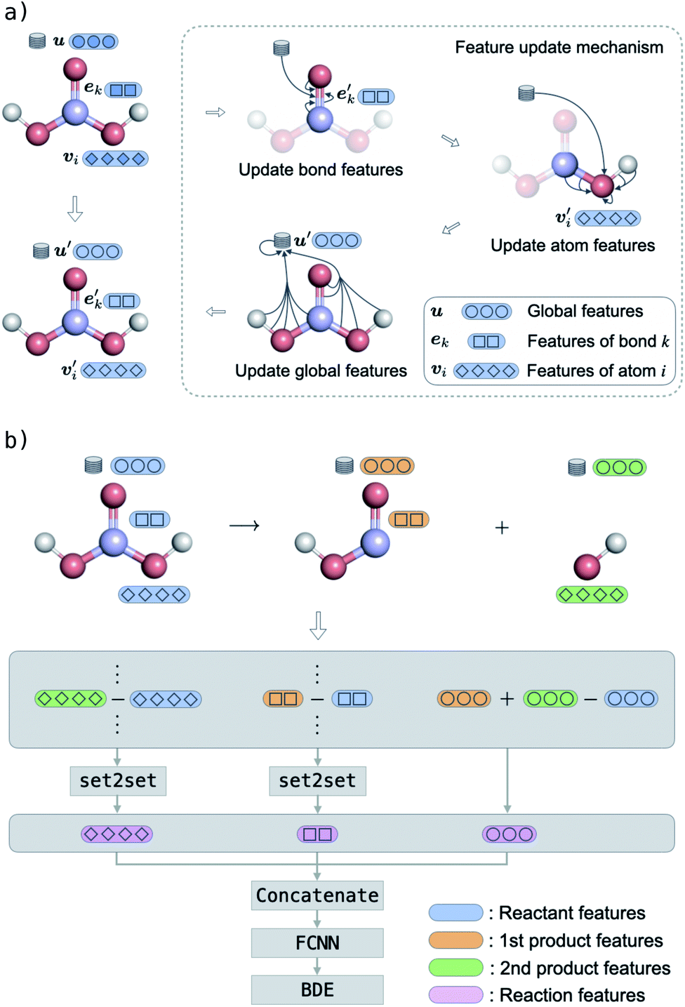 | ||
| Fig. 1 Schematic illustration of the BonDNet model for the prediction of bond dissociation energies (BDEs). (a) Graph-to-graph module to learn molecular representations. First, bond features are updated using messages passed from the two atoms forming the bond, the global state, and the bond itself. Similarly, atom features and global features are updated in sequence according to the messages passed among atoms, bonds, and the global state. This module is typically applied multiple times to learn better molecular representations. (b) Graph-to-property module to map molecular representations to a BDE. First, the features of the reactant are subtracted from the products; then the difference features are concatenated to form a representation of the reaction; and finally the representation of the reaction is mapped to the BDE via a fully connected neural network (FCNN). | ||
The bond feature update in eqn (4) and the atom feature update in eqn (5) pass messages based on the connectivity of the molecular graph, and the information exchange is thus inherently localized. To enable long-range interactions, we can compose multiple g2g modules together, taking the output of one module as the input for another module. For example, with four stacked g2g modules, the hydrogens of the H2CO3 molecule shown in Fig. 1a can interact because each g2g module lets an atom “see” other atoms one bond away from it. However, this is not realistic for large molecules where a large number of g2g modules would be needed to let all atoms interact as such an approach would make the model too deep to be effectively trained. This long-range interaction problem is addressed by the global feature update in eqn (7). In addition to encoding molecule-level information, the global features also serve as a central memory bank to facilitate long-range interaction. The bond and atom messages are aggregated to the memory bank in each g2g module and then disseminated from the memory bank to all bonds and atoms in the next g2g module. As a result, starting from the second g2g module, an atom or a bond can interact with all other atoms and bonds in the molecule. Our tests show that, with the help of the global features, three g2g modules are sufficient to learn good molecular representations.
2.2 Graph-to-property module
As discussed in Section 1, to build a general machine learning model for the prediction of both homolytic and heterolytic BDEs for molecules of any charge, one must take into consideration both the reactant and the products. Using the g2g module, we are able to describe single molecules of any charge. The key challenge is then to construct a representation for a reaction using both the reactant and products, a representation that should emphasize the breaking bond and its local environment.Our approach is illustrated in Fig. 1b. First, we stack multiple g2g modules together (a later module takes as input the output of a former module) and apply them to the reactant and products to obtain a better molecular representation for each of them. The number of g2g modules is determined via a hyperparameter search based on the model performance on the validation set (see Table S4 in the ESI†). We then take the differences of the features of each atom, each bond, and the global state between the products and the reactant:
 | (8) |
 is the feature vector of atom i in the product, and a similar explanation applies for the other terms appearing on the right-hand side of eqn (8). Upon bond dissociation, all atoms in the reactant are present in either the first product or the second product, and thus we can compute the difference feature for each atom. However, the breaking bond only exists in the reactant and not in the products. Thus, the breaking bond's product feature is set to a zero vector, i.e. its difference feature is equal to its negative reactant feature. Calculating the difference features requires atom mapping between the products and the reactant, which can be readily obtained via graph isomorphism. Next, we apply the set-to-set (set2set) model59 to aggregate the set of atom difference feature vectors {Δv'i} into a single vector,
  Similarly, set2set is applied to the bond difference feature vectors:
  Note that set2set is not applied to the global difference features since there is only one global difference feature vector for the reaction. The set2set model is invariant to permutation of atom/bond indices, and it is chosen over simply summing/averaging the difference features because it has more expressive power.39 After the set2set model, the atom, bond, and global difference feature vectors are concatenated to form a representation of the reaction,
| r = Δv′‖Δe′‖Δu′, | (9) |
The key aspect of our approach is to represent a bond dissociation reaction with difference features. Operating on the difference features has several advantages. First, they are obtained by subtracting the features of the reactant from the products, equivalent to how a BDE is computed from the energies of the products and the reactant. Second, since atoms and bonds far away from the breaking bond in the reactant and the products tend to have similar feature values,53,54 the difference features deviate significantly from zero only for atoms and bonds near the breaking bond. This enables the model to focus on the breaking bond and its surrounding environment, consistent with the chemical intuition that a BDE depends on the relatively local environment of the bond.
2.3 Input features
There are a number of atom, bond, and global raw features suitable as input for BonDNet, such as atom type, ring status of a bond, and molecular charge. A major consideration in choosing the features is that they should require little effort to obtain and do not require a quantum chemical calculation. Thus, we ignore geometric information such as bond length and bond angle which would not be available for new molecules for which the BDEs are to be predicted. For the same reason, we include the total charge of a molecule as a global feature instead of atomic partial charges (e.g. the restrained electrostatic potential (RESP) partial charge60) as atom features. A summary of the chosen input features is given in Tables S2 and S3 in the ESI,† and they are all generated with RDKit.61 The atom, bond, and global feature vectors typically do not have the same length, and thus linear transformations are applied to unify their length before passing them to BonDNet.2.4 Dataset and model training
There are two publicly available BDE datasets constructed from quantum chemical calculations: (1) the ZINC BDE dataset2 for the subset of “fragment-like” molecules in the ZINC database,62,63 and (2) the PubChem BDE dataset3 for CxHyOzNm molecules in the PubChem compound database.64 Both datasets only contain homolytic BDEs for neutral molecules. Using a novel framework for high-throughput simulation of charged and radical molecules,65 we constructed a new dataset consisting of over 60000 unique homolytic and heterolytic bond dissociations of neutral and charged molecules and their unique fragments, motivated by the need to understand reactivity in energy storage devices with organic electrolytes. (See the Datasets section in the ESI† for details on how the dataset is constructed.) This bond dissociation of neutral and charged molecules (BDNCM) dataset contains organic and inorganic species, closed-shell and radical molecules, molecules coordinated with metal ions, and molecules of charge −1, 0, and +1, all in the presence of an implicit solvent environment. (We note that BonDNet is a general model that can be applied to molecules of any charge, although we demonstrate its capabilities here with molecules of charge −1, 0, and +1.) See Table S1 in the ESI† for a summary of the three datasets.
Each dataset is split into three subsets for training, validation, and testing with a split ratio of 8:1:1. We optimize all model parameters in an end-to-end fashion using the training set, select hyperparameters based on the performance on the validation set, and report results on the test set unless otherwise stated. The model is implemented in Python using DGL66 with the PyTorch67 backend. To facilitate the training, we add a batch normalization (BN) layer68 and a dropout layer69 before the ReLU activation functions in eqn (4), (5) and (7). We train the model with the Adam optimizer to minimize a mean-squared-error loss function with a mini-batch size of 100. The learning rate is set to 0.001 at the start and is reduced if the validation error does not decrease for 50 epochs with a reducing rate of 0.5. The training stops when the validation error does not decrease for 150 epochs, and the optimization is allowed to run for a maximum of 1000 epochs. The optimal hyperparameters are obtained using a grid search and are given in Table S4 in the ESI.†
3 Results and discussion
3.1 Model performance
BonDNet outperforms previous models on homolytic BDEs for neutral molecules by a substantial margin. It also achieves a mean absolute error (MAE) significantly below the chemical accuracy on our BDNCM dataset of homolytic and heterolytic BDEs for both neutral and charged molecules.The mean absolute errors (MAEs) of BDEs predicted by BonDNet are presented in Table 1. The standard deviations are obtained by running the model five times with different data splits. Also included are MAEs by two other machine learning models: (1) ALFABET3 for the PubChem BDE dataset and (2) ANN2 for the ZINC BDE dataset. The ALFABET model is a GNN and the ANN model is an associate neural network trained on manually crafted features. MAEs by BonDNet are far below the chemical accuracy of 0.043 eV (i.e. 1 kcal mol−1)49 for both the BDNCM and PubChem BDE datasets. Although both BonDNet and ALFABET are GNN models, BonDNet outperforms ALFABET by 20% for the PubChem BDE dataset. BonDNet does not perform as well for the ZINC BDE dataset, with an MAE of about twice the chemical accuracy. One plausible explanation is that the ZINC BDE dataset is much smaller than the other two datasets (it consists of 16626 BDEs, only 5.7% the size of the PubChem BDE dataset); another could be that the reference BDE values in this dataset are less reliable and consistent, perhaps because the molecular geometries are optimized using a semiempirical tight-binding method as opposed to the DFT methods employed in the other two datasets. Nevertheless, BonDNet still achieves a 30% performance boost compared with the ANN model.
| BDNCM | PubChem | ZINC | |
|---|---|---|---|
| a MAEs are reported in eV. | |||
| BonDNet | 0.0221 ± 0.0026 | 0.0204 ± 0.0002 | 0.1013 ± 0.0076 |
| ALFABET | 0.0252 | ||
| ANN | 0.1453 | ||
To briefly test the transferability of BonDNet, we applied it predict the BDEs of a set of 82 drug-like molecules that are much larger than the molecules in the PubChem training set. The MAE for the drug-like molecules is 0.0460 eV (about twice the value of the MAE for the PubChem test set 0.0204 eV), which is acceptable considering that the drug-like molecules are much larger than the molecules in the PubChem dataset, and considering that this error is still roughly equal to chemical accuracy. See Fig. S2 in the ESI† for individual predictions.
As discussed in Section 1, it is possible to construct a machine learning model for the prediction of homolytic BDEs for neutral molecules based only on the reactants. For example, given the molecular graph G = (E,V) of a reactant (with no global features), we can update the atom and bond features with a procedure similar to the g2g module and then map the updated bond features to BDEs. In fact, ALFABET3 is such a model. In contrast, BonDNet (1) introduces global features to encode molecule-level information and (2) takes advantage of the chemically inspired difference features between the products and the reactant to represent a bond dissociation reaction.
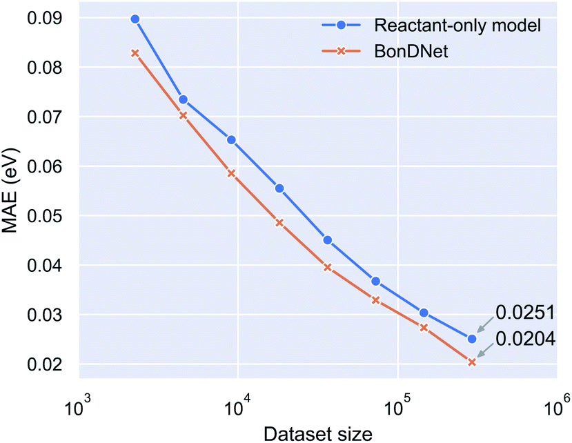
To determine whether it is the inclusion of global features or the use of difference features that allows BonDNet to perform better than ALFABET, we conducted an ablation analysis by training a reactant-only model and testing its performance on the PubChem BDE dataset. The reactant-only model sits between ALFABET and BonDNet. It is effectively the same as ALFABET except that it includes global features which are not present in ALFABET. Compared with BonDNet, the reactant-only model uses reactant features instead of the difference features between the products and the reactant. (See Table S5 in the ESI† for architectural details of the reactant-only model.) The reactant-only model achieves an MAE of 0.0251 eV for the PubChem BDE dataset, virtually the same as ALFABET (see Table 1), suggesting that the difference features are responsible for the superior performance of BonDNet. In addition to the whole PubChem BDE dataset, we also trained on randomly selected 1/2, 1/4, …, 1/128 subsets. Fig. 2 shows the MAE versus dataset size relation. We see that BonDNet performs better than the reactant-only model across a range of dataset sizes, small or large. The trend suggests that the accuracy of both models can be further improved when more data becomes available.
 | ||
| Fig. 2 Mean absolute error (MAE) of model prediction versus the size of the dataset used for training the model. BonDNet makes predictions based on the difference of the features between the products and the reactant of a bond dissociation reaction, while the reactant-only model only uses the reactant features. | ||
BonDNet is a general model capable of learning any type of BDEs. To obtain a deeper understanding of its behavior on complex datasets, we provide a more fine-grained performance analysis on the newly generated BDNCM dataset consisting of both homolytic and heterolytic BDEs for neutral and charged molecules.
Fig. 3a shows the BDEs predicted by BonDNet versus the reference values from quantum chemical computations. The prediction closely follows the reference along the diagonal line, yielding good results in a range of BDEs from −5 eV to 20 eV. Fig. 3b shows a distribution of the prediction error defined as the difference between the predicted BDE and the reference BDE. The prediction errors are tightly localized around 0, although there are a few larger ones which can be seen more clearly in the inset of Fig. 3b where the vertical axis is plotted on a log scale. We analyzed the reactions for which the magnitude of the prediction error is larger than 0.43 eV (10 times the chemical accuracy) and found that these reactions can be broadly categorized into two groups. First, some types of reactions are underrepresented in the dataset. It is expected that a machine learning model such as BonDNet cannot provide good predictions for such underrepresented data. Second, most reactions with large prediction errors are more complex than one-bond dissociation. For example, when breaking a bond leads to the spontaneous change of a neighboring single bond to a double bond. Such a change would substantially alter the reference BDE, adding complexity that BonDNet is not yet designed to deal with. The reactions with the 10 largest prediction errors are given in Fig. S1 in the ESI,† together with an explanation for each of them.
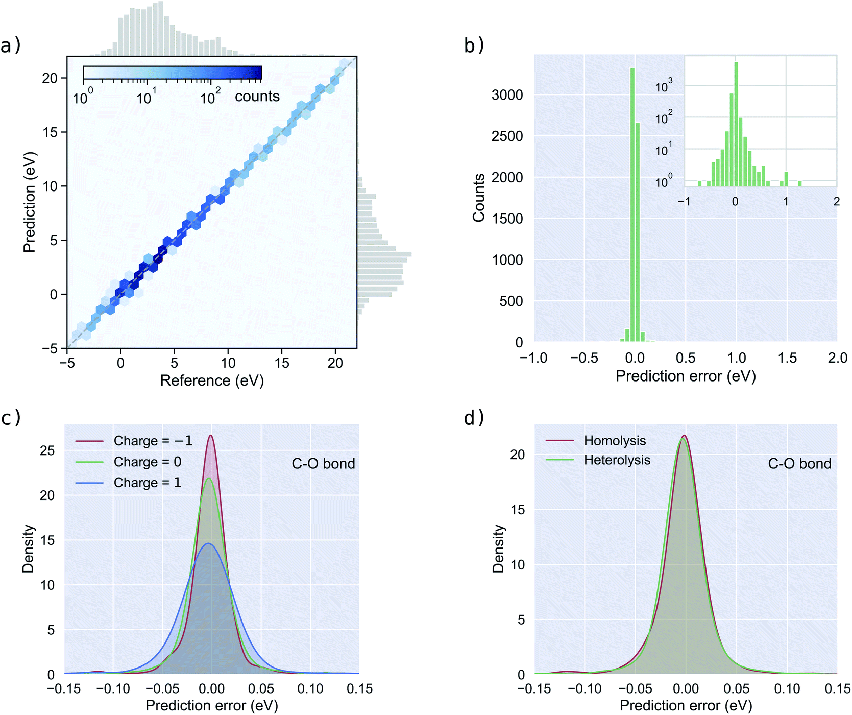 | ||
| Fig. 3 Performance of BonDNet on the BDNCM dataset. (a) BDEs predicted by BonDNet versus reference values computed from quantum chemistry; (b) histogram of the prediction error (difference between the prediction and the reference); (c) distribution of the prediction error in C–O bonds by reactant charge; and (d) distribution of the prediction error in C–O bonds by bond dissociation type. | ||
Table 2 presents the MAEs and bond counts by the type of the breaking bond for both the training set and test set. BonDNet makes predictions almost equally well for all types of bonds in the training set irrespective of their counts. However, this does not mean the model would generalize equally well for unseen data (e.g. the test set) of different bond types. In fact, if a bond type has more instances in the training set, the model can more easily learn the corresponding underlying chemistry; thus, the model would generalize better for unseen data of this bond type. This can be seen from the test set MAEs in Table 2: the MAE decreases in general as the bond counts increase. As a specific example, although the training MAE for C–O and F→Li+ bonds are almost the same, the test MAE for C–O bonds is about only one third of that for F→Li+ bonds because the dataset has many more BDEs for C–O bonds. This data imbalance problem can be solved by collecting more BDEs for the underrepresented bonds in the future.
| Bond type | MAE (train) | Counts (train) | MAE (test) | Counts (test) |
|---|---|---|---|---|
| a MAEs are reported in eV; the arrow “→” denotes a coordinate bond. | ||||
| C–O | 0.0050 | 17037 |
0.0185 | 2152 |
| C–H | 0.0045 | 12920 |
0.0189 | 1545 |
| C–C | 0.0047 | 11774 |
0.0177 | 1557 |
| O→Li+ | 0.0046 | 3868 | 0.0272 | 474 |
| H–O | 0.0046 | 2313 | 0.0197 | 270 |
| C–F | 0.0049 | 1890 | 0.0269 | 228 |
| C→Li+ | 0.0051 | 1070 | 0.0496 | 138 |
| F→Li+ | 0.0055 | 437 | 0.0539 | 54 |
| O–F | 0.0131 | 75 | 0.0409 | 8 |
| O–O | 0.0137 | 51 | 0.4886 | 5 |
| H–F | 0.0181 | 7 | — | 0 |
| F–F | 0.0031 | 4 | — | 0 |
| H–H | 0.0088 | 4 | — | 0 |
Next, we assess how BonDNet performs with respect to the reactant charge using C–O bonds as an example. (Results for other bond types are given in Fig. S3 and S4 in the ESI.†) We divide the C–O bonds into three groups according to the charge of the reactants and plot the distribution of the prediction error in Fig. 3c. For all three groups, the prediction error is centered around 0. The prediction error for −1 charged molecules is somewhat more localized than for neutral molecules. As a result, the MAE for −1 charged molecules is smaller than for neutral molecules, as can be seen in Table 3. For the same reason, the MAEs for both −1 charged and neutral molecules are smaller than the MAE for +1 charged molecules. Nevertheless, these differences are not large, and BonDNet is able to accurately predict the BDEs for molecules of different charges. In a similar manner, we assess the performance of BonDNet with respect to the bond dissociation type: homolysis or heterolysis. The difference in the distributions of the prediction error (Fig. 3d) is negligible; the same can be said for the MAEs (Table 3), demonstrating that BonDNet is able to accurately predict both homolytic and heterolytic BDEs.
| MAE (eV) | Counts | ||
|---|---|---|---|
| Charge | −1 | 0.0146 | 787 |
| 0 | 0.0178 | 890 | |
| 1 | 0.0265 | 475 |
| Dissociation type | Homolysis | 0.0189 | 1373 |
| Heterolysis | 0.0178 | 779 |
3.2 Analysis of the learning process
Deep learning models can typically achieve good performance when trained on reasonably large datasets, but they are oftentimes regarded as “black boxes” because it is not easy to interpret what a model learns by mapping it to scientific domain knowledge and how a model learns by adjusting its parameters.42 By design, we tried to incorporate chemical insights into the architecture of BonDNet. For example, the difference of the features between the products and the reactant is taken to construct the feature vector representing a bond dissociation reaction, which is similar to how a BDE is computed from the energies of the products and the reactant. In this section, we further explore how BonDNet learns by adjusting its parameters to capture the underlying nature of chemical bonding in the data via the analysis of the patterns in the learned features.First, we look at the learned representations of the bond dissociation reactions. This provides us with an idea of how the model learns to map the inputs to the BDE predictions. For easier visual discovery of patterns, we embed the high-dimensional difference feature vector in eqn (9) for each reaction into a two-dimensional (2D) space by the uniform manifold approximation and projection (UMAP) method.70Fig. 4 shows the embedding for the BDNCM test set. In general, points that are close together in the 2D embedded space are similar in the original vector space. Therefore, since reactions with similar BDEs are close to each other in the embedded 2D space (Fig. 4a), their feature vectors are similar to each other. Note that all model parameters are optimized in an end-to-end fashion, where the g2g module and the g2p module work together to achieve the goal of reproducing the reference BDEs in the training set. Consequently, the feature vectors representing the reactions are adapted in accordance with the BDEs during the training process. Fig. 4b shows that reactions with the same type of breaking bond tend to “cluster” together, but there can be multiple faraway clusters for each bond type. The former is simply because reactions with the same type of breaking bond are similar to each other as we would expect. The latter, however, is because the surrounding environment of the bonds and/or the global state (e.g. total charge) of the molecules are different such that the model assigns distinctive feature vectors to them, in spite of being the same bond type. These observations suggest that the model “listens” to both the input (e.g. bond type) and the target (BDE) and learns by transforming the feature vectors to be aligned with them.
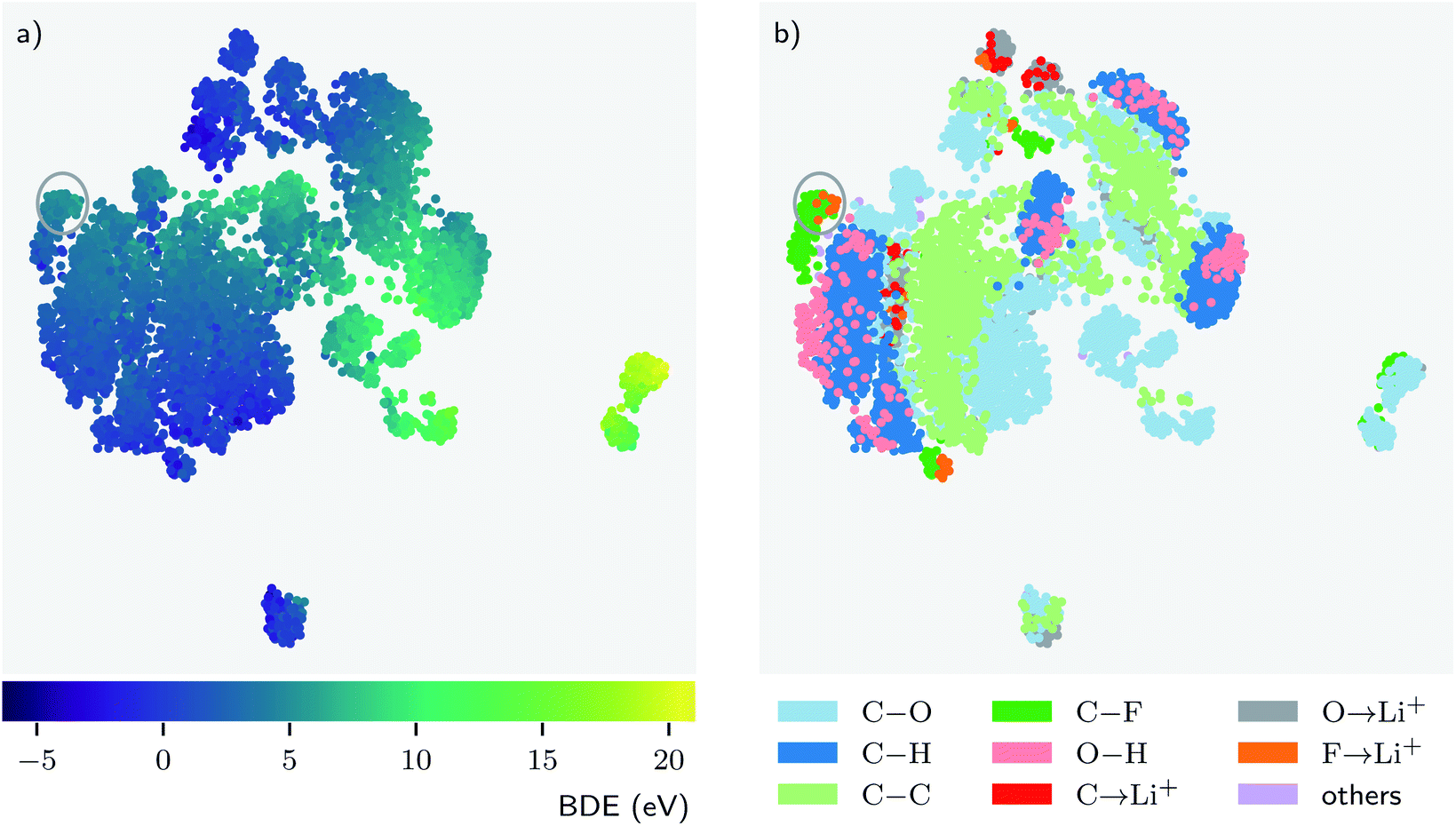 | ||
| Fig. 4 Embedding of the high-dimensional feature vectors representing the bond dissociation reactions into a two-dimensional space. The embedding is obtained using the uniform manifold approximation and projection (UMAP) technique. Each data point in the plot represents one bond dissociation reaction and the points are colored according to their (a) BDE value and (b) bond type. The arrow “→” denotes a coordinate bond. | ||
Furthermore, the patterns in the data yield chemical insights that may align with common chemical knowledge or, in some cases, challenge chemical intuition.42,71,72 Such insight would provide new perspectives on the data and thus help us to better understand the system under study. For example, in Fig. 4b we see that O–H bonds (pink) are always associated with C–H bonds (dark blue). This means that, despite the unique nature of O–H bonds, the model finds them to be fairly similar to C–H bonds. However, from the perspective of the learning model this is unsurprising because both O–H and C–H are covalent bonds formed with hydrogen atoms, and more importantly, unlike other atoms, hydrogen can only form one bond. The behavior of bonds formed with lithium is more interesting. We might expect F→Li+, C→Li+, and O→Li+ bonds to be similar because they are all coordinate bonds involving a lithium ion Li+. This is indeed the case for some F→Li+ bonds, as can be seen from the upper part of Fig. 4b where the F→Li+ (orange), C→Li+ (red), and O→Li+ (gray) bonds are close to each other. Surprisingly, there are a fair number of F→Li+ bonds (orange) deemed more similar to C–F bonds (dark green) than to the other coordinate bonds. There are two major reasons for this counterintuitive behavior. First, both F→Li+ and C–F are bonds formed with F. Second, the F→Li+ bonds have a wide spectrum of BDEs (−0.2 to 21.1 eV in the dataset), and some of them have BDEs more close to the C–F bonds. Such close BDEs result in the adaption of the feature vectors corresponding to these F→Li+ bonds towards the feature vectors of the C–F bonds during the training. For example, the F→Li+ and C–F bonds in the circle have very similar energies and, obviously, they are close to each other in the embedded 2D space.
In addition to the reaction-level difference features in the g2p module, each bond has its own features in each g2g module. To investigate how the bond features evolve in the learning process, we calculate the similarity between bond pairs by measuring the Pearson correlation coefficient between their feature vectors and observe how the similarity changes in different layers of BonDNet (a layer means a g2g module). Taking the fluorine-substituted lithium butylene dicarbonate molecule (F-LBDC) in the BDNCM dataset as an example (Fig. 5b), Fig. 5a shows the heatmap of the bond similarity matrix for various layers of BonDNet. The input bond features only include “whether a bond is in a ring”, “ring size”, and “whether a bond is a coordinate bond” (see Table S2 in the ESI† for more information on input features). As a result, the bond similarity for input features (layer 0) aggregates into two groups mainly based on the “whether a bond is in a ring” information. Moreover, the bonds in rings (bonds 1, 2, 3, and 4 in Fig. 5b) further aggregate into two subgroups according to “whether a bond is a coordinate bond.” As the learning proceeds, the bond similarity heatmap presents a distinctive pattern in later layers. For example, were it not for the fluorine substitution, bonds 9 and 11 would exhibit a similarity score of 1 in all layers due to the symmetry in the LBDC molecule. However, bond 11 in layer 3 is more similar to bond 10 (correlation score 0.92) than to bond 9 (correlation score 0.81), in agreement with our chemical intuition that the fluorine atom substantially impacts the properties of its neighboring bonds.
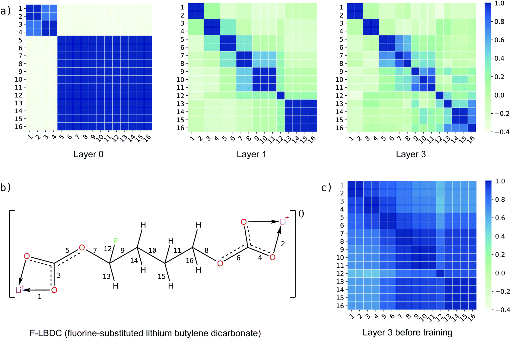 | ||
| Fig. 5 Bond similarity for the fluorine-substituted lithium butylene dicarbonate molecule (F-LBDC) measured as the Pearson correlation coefficient between the bond feature vectors. (a) Heatmap of the bond similarity matrix for the input features (layer 0), first g2g module (layer 1), and last g2g module (layer 3); (b) the F-LBDC molecule, where identical bonds are labelled only once (the arrow “→” denotes a coordinate bond); and (c) heatmap of the bond similarity matrix for the last g2g module (layer 3) before training the model. | ||
As a comparison, Fig. 5c displays the heatmap of the bond similarity matrix for layer 3 before training the BonDNet model. There is hardly any visual pattern in the heatmap that is in strong agreement with the chemical structure of the F-LBDC molecule. This demonstrates that BonDNet has learned to transform the raw input features into more refined features via the exchange of information among atoms, bonds, and the global state in the g2g module. More importantly, the refined features are in agreement with our understanding of the molecules, suggesting that BonDNet learns to predict the BDE by trying to understand the underlying chemical rules.
4 Conclusions
By incorporating chemical insights into the model architecture via global features and difference features, we have designed a GNN model for accurate prediction of BDEs. Our BonDNet model learns by adjusting its parameters to capture the underlying nature of chemical bonding in the data, and it outperforms previous state-of-the-art models in prediction accuracy. BonDNet is the very first machine learning model capable of predicting both homolytic and heterolytic BDEs for molecules of any charge. An interface to use the developed model to make predictions is provided via binder55 and can be accessed at https://github.com/mjwen/bondnet. A user can simply provide a molecule of interest (e.g. as a SMILES string or connectivity matrix along with the total molecular charge), and the tool will return the BDEs of all the bonds in the molecule. As an intrinsic property of bond dissociation reactions, BDEs and their relative strengths are crucial in understanding many chemical processes, such as drug metabolism, biofuel combustion, photochemical decontamination of water pollutants, formation of side products in batteries and solar cells, and so forth. We expect applications involving such processes will benefit from our model to conduct fast and accurate high-throughput screening for critical reactions and molecules based on BDEs.BonDNet does not take as input any geometric information of molecules, and thus stereoisomers (e.g. cis/trans isomers) cannot be distinguished. This, however, could be addressed by directly encoding the isomerism information into the atom, bond, and global features without explicitly using the geometric information, which we leave for future investigation.
In essence, BonDNet is a model that represents chemical reactions using molecular features of both the reactants and the products. Therefore, our approach is not limited to just predicting BDEs but could be applied to learn other reaction properties such as activation energy, retrosynthesis chemical reactivity, and reaction conditions (e.g. temperature and solvents). Such capabilities would require little to no modification of the current model besides modifying the training target to be another property of interest. Future generation of large quantitative datasets through high-throughput experimentation and/or quantum computational chemistry methods will thus enable the adoption of BonDNet and similar methods for rapid and accurate prediction of such properties.
Code availability
The BonDNet graph neural network model is released as an open-source repository at https://github.com/mjwen/bondnet.Conflicts of interest
There are no conflicts to declare.Acknowledgements
The method development of BonDNet was collaboratively supported by the Joint Center for Energy Storage Research, an Energy Innovation Hub funded by the US Department of Energy, Office of Science, Basic Energy Sciences as well as by the Silicon Electrolyte Interface Stabilization (SEISTA) Consortium directed by Brian Cunningham under the Assistant Secretary for Energy Efficiency and Renewable Energy, Office of Vehicle Technologies Program of the U.S. Department of Energy, Contract No. DE-AC02-05CH11231. Data production was supported by the Battery Materials Research (BMR) program directed by Tien Duong under the Assistant Secretary for Energy Efficiency and Renewable Energy, Office of Vehicle Technologies Program of the U.S. Department of Energy, Contract DE-AC02-05CH11231. Computational resources were provided by the National Energy Research Scientific Computing Center (NERSC), a U.S. Department of Energy Office of Science User Facility under Contract No. DE-AC02-05CH11231, and by the Department of Energy's Office of Energy Efficiency and Renewable Energy (located at the National Renewable Energy Laboratory). This research also used the Lawrencium computational cluster resource provided by the IT Division at the Lawrence Berkeley National Laboratory (Supported by the Director, Office of Science, Office of Basic Energy Sciences, of the U.S. Department of Energy under Contract No. DE-AC02-05CH11231).Notes and references
- K. Schmidt-Rohr, J. Chem. Educ., 2015, 92, 2094–2099 CrossRef CAS.
- X. Qu, D. A. Latino and J. Aires-de Sousa, J. Cheminf., 2013, 5, 34 CAS.
- P. C. S. John, Y. Guan, Y. Kim, S. Kim and R. S. Paton, Nat. Commun., 2020, 11, 2328 CrossRef PubMed.
- C. W. Coley, L. Rogers, W. H. Green and K. F. Jensen, ACS Cent. Sci., 2017, 3, 1237–1245 CrossRef CAS.
- M. H. S. Segler and M. P. Waller, Chem.–Eur. J., 2017, 23, 5966–5971 CrossRef CAS.
- C. W. Coley, W. H. Green and K. F. Jensen, Acc. Chem. Res., 2018, 51, 1281–1289 CrossRef CAS PubMed.
- L. Ji, A. S. Faponle, M. G. Quesne, M. A. Sainna, J. Zhang, A. Franke, D. Kumar, R. van Eldik, W. Liu and S. P. de Visser, Chem.–Eur. J., 2015, 21, 8973 CrossRef.
- K. Kohse-Höinghaus, P. Oßwald, T. A. Cool, T. Kasper, N. Hansen, F. Qi, C. K. Westbrook and P. R. Westmoreland, Angew. Chem., Int. Ed., 2010, 49, 3572–3597 CrossRef PubMed.
- J. L. Bao, R. Meana-Pañeda and D. G. Truhlar, Chem. Sci., 2015, 6, 5866–5881 RSC.
- M. Freccero, M. Fagnoni and A. Albini, J. Am. Chem. Soc., 2003, 125, 13182–13190 CrossRef CAS.
- B. Lee, J. Yoo and K. Kang, Chem. Sci., 2020, 11, 7813–7822 RSC.
- R. P. Bell, Proc. R. Soc. London, Ser. A, 1936, 154, 414–429 Search PubMed.
- M. G. Evans and M. Polanyi, Trans. Faraday Soc., 1936, 32, 1333 RSC.
- P. Houston, Chemical Kinetics and Reaction Dynamics, Dover Publications, 2012 Search PubMed.
- M. Silberberg, Chemistry: The Molecular Nature of Matter and Change, McGraw-Hill Companies, Incorporated, 2008 Search PubMed.
- T. Brown, H. LeMay, B. Bursten, C. Murphy, P. Woodward and M. Stoltzfus, Chemistry: The Central Science, Pearson Education, 2017 Search PubMed.
- F. G. Bordwell, J. P. Cheng and J. A. Harrelson, J. Am. Chem. Soc., 1988, 110, 1229–1231 CrossRef CAS.
- D. C. Miller, K. T. Tarantino and R. R. Knowles, Topics in Current Chemistry Collections, Springer, 2016, pp. 145–203 Search PubMed.
- C. F. Wise and J. M. Mayer, J. Am. Chem. Soc., 2019, 141, 14971–14975 CrossRef CAS PubMed.
- W. Luo, C. Mao, P. Ji, J.-Y. Wu, J.-D. Yang and J.-P. Cheng, Chem. Sci., 2020, 11, 3365–3370 RSC.
- X. Li, X. Xu, X. You and D. G. Truhlar, J. Phys. Chem. A, 2016, 120, 4025–4036 CrossRef CAS PubMed.
- A. Nazemi and T. R. Cundari, Inorg. Chem., 2017, 56, 12319–12327 CrossRef CAS PubMed.
- F. Häse, C. Kreisbeck and A. Aspuru-Guzik, Chem. Sci., 2017, 8, 8419–8426 RSC.
- B. Liu, B. Ramsundar, P. Kawthekar, J. Shi, J. Gomes, Q. L. Nguyen, S. Ho, J. Sloane, P. Wender and V. Pande, ACS Cent. Sci., 2017, 3, 1103–1113 CrossRef CAS PubMed.
- J. N. Wei, D. Duvenaud and A. Aspuru-Guzik, ACS Cent. Sci., 2016, 2, 725–732 CrossRef CAS PubMed.
- C. W. Coley, R. Barzilay, T. S. Jaakkola, W. H. Green and K. F. Jensen, ACS Cent. Sci., 2017, 3, 434–443 CrossRef CAS PubMed.
- P. Schwaller, T. Gaudin, D. Lányi, C. Bekas and T. Laino, Chem. Sci., 2018, 9, 6091–6098 RSC.
- M. H. S. Segler, M. Preuss and M. P. Waller, Nature, 2018, 555, 604–610 CrossRef CAS PubMed.
- R. Gómez-Bombarelli, J. N. Wei, D. Duvenaud, J. M. Hernández-Lobato, B. Sánchez-Lengeling, D. Sheberla, J. Aguilera-Iparraguirre, T. D. Hirzel, R. P. Adams and A. Aspuru-Guzik, ACS Cent. Sci., 2018, 4, 268–276 CrossRef PubMed.
- B. Sanchez-Lengeling and A. Aspuru-Guzik, Science, 2018, 361, 360–365 CrossRef CAS PubMed.
- W. Jin, R. Barzilay and T. S. Jaakkola, Proceedings of the 35th International Conference on Machine Learning, 2018, pp. 2328–2337 Search PubMed.
- Z. Zhou, S. Kearnes, L. Li, R. N. Zare and P. Riley, Sci. Rep., 2019, 9, 1–10 Search PubMed.
- A. S. Christensen, L. A. Bratholm, F. A. Faber and O. A. von Lilienfeld, J. Chem. Phys., 2020, 152, 044107 CrossRef CAS PubMed.
- B. Huang and O. A. von Lilienfeld, Nat. Chem., 2020, 12, 945–951 CrossRef CAS PubMed.
- P. C. D. Hawkins, A. G. Skillman and A. Nicholls, J. Med. Chem., 2007, 50, 74–82 CrossRef CAS PubMed.
- D. Rogers and M. Hahn, J. Chem. Inf. Model., 2010, 50, 742–754 CrossRef CAS PubMed.
- J. P. Janet and H. J. Kulik, Chem. Sci., 2017, 8, 5137–5152 RSC.
- R. Todeschini, V. Consonni, R. Mannhold, H. Kubinyi and G. Folkers, Molecular Descriptors for Chemoinformatics: Volume I: Alphabetical Listing/Volume II: Appendices, References, Wiley, 2009 Search PubMed.
- J. Gilmer, S. S. Schoenholz, P. F. Riley, O. Vinyals and G. E. Dahl, Proceedings of the 34th International Conference on Machine Learning-Volume 70, 2017, pp. 1263–1272 Search PubMed.
- K. T. Schütt, H. E. Sauceda, P.-J. Kindermans, A. Tkatchenko and K.-R. Müller, J. Chem. Phys., 2018, 148, 241722 CrossRef PubMed.
- E. N. Feinberg, D. Sur, Z. Wu, B. E. Husic, H. Mai, Y. Li, S. Sun, J. Yang, B. Ramsundar and V. S. Pande, ACS Cent. Sci., 2018, 4, 1520–1530 CrossRef CAS PubMed.
- Z. Xiong, D. Wang, X. Liu, F. Zhong, X. Wan, X. Li, Z. Li, X. Luo, K. Chen, H. Jiang and M. Zheng, J. Med. Chem., 2019, 63(16), 8749–8760 CrossRef PubMed.
- K. Yang, K. Swanson, W. Jin, C. Coley, P. Eiden, H. Gao, A. Guzman-Perez, T. Hopper, B. P. Kelley, M. Aathea, A. Palmer, V. Settels, T. S. Jaakkola, K. F. Jensen and R. Barzilay, J. Chem. Inf. Model., 2019, 59, 3370–3388 CrossRef CAS PubMed.
- S. Kearnes, K. McCloskey, M. Berndl, V. Pande and P. Riley, J. Comput.-Aided Mol. Des., 2016, 30, 595–608 CrossRef CAS PubMed.
- Z. Wu, B. Ramsundar, E. N. Feinberg, J. Gomes, C. Geniesse, A. S. Pappu, K. Leswing and V. Pande, Chem. Sci., 2018, 9, 513–530 RSC.
- J. Klicpera, J. Groß and S. Günnemann, International Conference on Learning Representations (ICLR), 2020 Search PubMed.
- Y. Feng, L. Liu, J.-T. Wang, S.-W. Zhao and Q.-X. Guo, J. Org. Chem., 2004, 69, 3129–3138 CrossRef CAS PubMed.
- C. X. Xue, R. S. Zhang, H. X. Liu, X. J. Yao, M. C. Liu, Z. D. Hu and B. T. Fan, J. Chem. Inf. Comput. Sci., 2004, 44, 669–677 CrossRef CAS PubMed.
- F. A. Faber, L. Hutchison, B. Huang, J. Gilmer, S. S. Schoenholz, G. E. Dahl, O. Vinyals, S. Kearnes, P. F. Riley and O. A. von Lilienfeld, J. Chem. Theory Comput., 2017, 13, 5255–5264 CrossRef CAS PubMed.
- P. W. Battaglia, J. B. Hamrick, V. Bapst, A. Sanchez-Gonzalez, V. Zambaldi, M. Malinowski, A. Tacchetti, D. Raposo, A. Santoro, R. Faulkner, et al., 2018, arXiv preprint arXiv:1806.01261.
- C. Chen, W. Ye, Y. Zuo, C. Zheng and S. P. Ong, Chem. Mater., 2019, 31, 3564–3572 CrossRef CAS.
- N. Schneider, D. M. Lowe, R. A. Sayle and G. A. Landrum, J. Chem. Inf. Model., 2015, 55, 39–53 CrossRef CAS PubMed.
- C. W. Coley, W. Jin, L. Rogers, T. F. Jamison, T. S. Jaakkola, W. H. Green, R. Barzilay and K. F. Jensen, Chem. Sci., 2019, 10, 370–377 RSC.
- C. Grambow, L. Pattanaik and W. H. Green, J. Phys. Chem. Lett., 2020, 11(8), 2992–2997 CrossRef CAS PubMed.
- P. Jupyter, M. Bussonnier, J. Forde, J. Freeman, B. Granger, T. Head, C. Holdgraf, K. Kelley, G. Nalvarte, A. Osheroff, M. Pacer, Y. Panda, F. Perez, B. R. Kelley and C. Willing, Proceedings of the 17th Python in Science Conference, 2018, pp. 113–120 Search PubMed.
- X. Bresson and T. Laurent, 2017, arXiv preprint arXiv:1711.07553.
- V. P. Dwivedi, C. K. Joshi, T. Laurent, Y. Bengio and X. Bresson, 2020, arXiv preprint arXiv:2003.00982.
- I. Goodfellow, Y. Bengio and A. Courville, Deep learning, MIT Press, 2016 Search PubMed.
- O. Vinyals, S. Bengio and M. Kudlur, International Conference on Learning Representations (ICLR), 2016 Search PubMed.
- R. Woods and R. Chappelle, J. Mol. Struct.: THEOCHEM, 2000, 527, 149–156 CrossRef CAS.
- RDKit: Open-source cheminformatics, http://www.rdkit.org, accessed 2020-06-30 Search PubMed.
- J. J. Irwin, T. Sterling, M. M. Mysinger, E. S. Bolstad and R. G. Coleman, J. Chem. Inf. Model., 2012, 52, 1757–1768 CrossRef CAS PubMed.
- R. A. Carr, M. Congreve, C. W. Murray and D. C. Rees, Drug Discovery Today, 2005, 10, 987–992 CrossRef CAS PubMed.
- S. Kim, J. Chen, T. Cheng, A. Gindulyte, J. He, S. He, Q. Li, B. A. Shoemaker, P. A. Thiessen, B. Yu, L. Zaslavsky, J. Zhang and E. E. Bolton, Nucleic Acids Res., 2019, 47, D1102–D1109 CrossRef PubMed.
- S. M. Blau, E. W. C. Spotte-Smith, X. Xie, B. M. Wood, H. Patel, M. Wen, S. Dwaraknath and K. A. Persson, Quantum chemical calculations of lithium-ion battery electrolyte decomposition products and intermediates, 2020, unpublished.
- M. Wang, L. Yu, D. Zheng, Q. Gan, Y. Gai, Z. Ye, M. Li, J. Zhou, Q. Huang, C. Ma, Z. Huang, Q. Guo, H. Zhang, H. Lin, J. Zhao, J. Li, A. J. Smola and Z. Zhang, ICLR Workshop on Representation Learning on Graphs and Manifolds, 2019 Search PubMed.
- A. Paszke, S. Gross, F. Massa, A. Lerer, J. Bradbury, G. Chanan, T. Killeen, Z. Lin, N. Gimelshein, L. Antiga, et al., Advances in neural information processing systems, 2019, pp. 8026–8037 Search PubMed.
- S. Ioffe and C. Szegedy, Proceedings of the 32nd International Conference on International Conference on Machine Learning – Volume 37, 2015, p. 448–456 Search PubMed.
- N. Srivastava, G. Hinton, A. Krizhevsky, I. Sutskever and R. Salakhutdinov, J. Mach. Learn. Res., 2014, 15, 1929–1958 Search PubMed.
- L. McInnes, J. Healy, N. Saul and L. Großberger, J. Open Source Softw., 2018, 3, 861 CrossRef.
- K. T. Butler, D. W. Davies, H. Cartwright, O. Isayev and A. Walsh, Nature, 2018, 559, 547–555 CrossRef CAS PubMed.
- F. Häse, I. F. Galván, A. Aspuru-Guzik, R. Lindh and M. Vacher, Chem. Sci., 2019, 10, 2298–2307 RSC.
Footnotes |
| † Electronic supplementary information (ESI) available: Dataset description, raw input features, model hyperparameters, and additional error analysis. See DOI: 10.1039/d0sc05251e |
| ‡ It should be noted that, if the breaking bond is part of a ring, only one product will be formed. Without loss of generality, we assume the reactant cleaves into two products in this paper. |
| This journal is © The Royal Society of Chemistry 2021 |