 Open Access Article
 This Open Access Article is licensed under a
 Creative Commons Attribution 3.0 Unported Licence
Sources of non-methane hydrocarbons in surface air in Delhi, India†
Gareth J.
Stewart
a,
Beth S.
Nelson
 a,
Will S.
Drysdale
a,
W. Joe F.
Acton
b,
Adam R.
Vaughan
a,
James R.
Hopkins
ac,
Rachel E.
Dunmore
a,
C. Nicholas
Hewitt
b,
Eiko
Nemitz
d,
Neil
Mullinger
d,
Ben
Langford
d,
Shivani
e,
Ernesto
Reyes-Villegas
f,
Ranu
Gadi
e,
Andrew R.
Rickard
ac,
James D.
Lee
ac and
Jacqueline F.
Hamilton
*a
a,
Will S.
Drysdale
a,
W. Joe F.
Acton
b,
Adam R.
Vaughan
a,
James R.
Hopkins
ac,
Rachel E.
Dunmore
a,
C. Nicholas
Hewitt
b,
Eiko
Nemitz
d,
Neil
Mullinger
d,
Ben
Langford
d,
Shivani
e,
Ernesto
Reyes-Villegas
f,
Ranu
Gadi
e,
Andrew R.
Rickard
ac,
James D.
Lee
ac and
Jacqueline F.
Hamilton
*a
aWolfson Atmospheric Chemistry Laboratories, Department of Chemistry, University of York, York, YO10 5DD, UK. E-mail: jacqui.hamilton@york.ac.uk
bLancaster Environment Centre, Lancaster University, Lancaster, LA1 4YQ, UK
cNational Centre for Atmospheric Science, University of York, York, YO10 5DD, UK
dUK Centre for Ecology and Hydrology, Bush Estate, Penicuik, EH26 0QB, UK
eIndira Gandhi Delhi Technical University for Women, Kashmiri Gate, New Delhi, Delhi 110006, India
fDepartment of Earth and Environmental Sciences, The University of Manchester, Manchester, M13 9PL, UK
First published on 13th August 2020
Abstract
Rapid economic growth and development have exacerbated air quality problems across India, driven by many poorly understood pollution sources and understanding their relative importance remains critical to characterising the key drivers of air pollution. A comprehensive suite of measurements of 90 non-methane hydrocarbons (NMHCs) (C2–C14), including 12 speciated monoterpenes and higher molecular weight monoaromatics, were made at an urban site in Old Delhi during the pre-monsoon (28-May to 05-Jun 2018) and post-monsoon (11 to 27-Oct 2018) seasons using dual-channel gas chromatography (DC-GC-FID) and two-dimensional gas chromatography (GC×GC-FID). Significantly higher mixing ratios of NMHCs were measured during the post-monsoon campaign, with a mean night-time enhancement of around 6. Like with NOx and CO, strong diurnal profiles were observed for all NMHCs, except isoprene, with very high NMHC mixing ratios between 35–1485 ppbv. The sum of mixing ratios of benzene, toluene, ethylbenzene and xylenes (BTEX) routinely exceeded 100 ppbv at night during the post-monsoon period, with a maximum measured mixing ratio of monoaromatic species of 370 ppbv. The mixing ratio of highly reactive monoterpenes peaked at around 6 ppbv in the post-monsoon campaign and correlated strongly with anthropogenic NMHCs, suggesting a strong non-biogenic source in Delhi. A detailed source apportionment study was conducted which included regression analysis to CO, acetylene and other NMHCs, hierarchical cluster analysis, EPA UNMIX 6.0, principal component analysis/absolute principal component scores (PCA/APCS) and comparison with NMHC ratios (benzene/toluene and i-/n-pentane) in ambient samples to liquid and solid fuels. These analyses suggested the primary source of anthropogenic NMHCs in Delhi was from traffic emissions (petrol and diesel), with average mixing ratio contributions from Unmix and PCA/APCS models of 38% from petrol, 14% from diesel and 32% from liquified petroleum gas (LPG) with a smaller contribution (16%) from solid fuel combustion. Detailed consideration of the underlying meteorology during the campaigns showed that the extreme night-time mixing ratios of NMHCs during the post-monsoon campaign were the result of emissions into a very shallow and stagnant boundary layer. The results of this study suggest that despite widespread open burning in India, traffic-related petrol and diesel emissions remain the key drivers of gas-phase urban air pollution in Delhi.
Introduction
Poor urban air quality is a major global public health concern, particularly in the developing world, as rapid urban growth has increased concentrations to harmful levels. This issue remains at the forefront of many governmental policies, as by 2050 approximately 66% of the global population are expected to live in urban environments.1 Globally, an estimated 4.2 million premature deaths were a result of poor ambient air quality in 2016,2 mainly caused by exposure to particulate matter (PM) and ozone (O3). NMHCs are key precursors to PM and O3 and some, such as aromatic species, are carcinogenic themselves.3 Globally biogenic NMHC emissions are the dominant source with an estimated flux of 377–760 TgC per year.4–6 However, anthropogenic emissions, which have been estimated to be 130–169 TgC per year,5,7,8 can be important drivers of poor air quality in densely populated urban environments.NMHC emissions from India are high and poorly understood, with emissions estimated to be the second largest in Asia, after China.9,10 Several emissions inventories have been produced for India, which included a range of NMHC sources.9,11–15 However, inventories remain hard to evaluate without knowledge of unaccounted for and unregulated sources and their strength.
Delhi (28°40′0′′N, 77°10′0′′E) had a population of around 29 million in 2018![[thin space (1/6-em)]](https://www.rsc.org/images/entities/char_2009.gif) 16 and has been ranked as the worst of 1600 cities in the world for air pollution, based on available data.17 The air quality index of Delhi is rarely considered good by international standards (see the ESI1†). As a result, 1/3 of adults and 2/3 of children in Delhi have experienced respiratory symptoms owing to poor air quality.18 NMHC pollution has been previously highlighted as coming from uncontrolled and unregulated sources in and surrounding Delhi and amplified by an unfavourable geographic location.19 NMHCs are a key driver of air pollution in Delhi: the composition of fine particulates (PM1) in Delhi has been found to be dominated by oxygenated organic aerosol which derives from NMHC precursors,20–22 whilst ozone production has been found to be in a regime where NOx emissions reduction, without simultaneous reduction in NMHCs, would lead to an increase.23
16 and has been ranked as the worst of 1600 cities in the world for air pollution, based on available data.17 The air quality index of Delhi is rarely considered good by international standards (see the ESI1†). As a result, 1/3 of adults and 2/3 of children in Delhi have experienced respiratory symptoms owing to poor air quality.18 NMHC pollution has been previously highlighted as coming from uncontrolled and unregulated sources in and surrounding Delhi and amplified by an unfavourable geographic location.19 NMHCs are a key driver of air pollution in Delhi: the composition of fine particulates (PM1) in Delhi has been found to be dominated by oxygenated organic aerosol which derives from NMHC precursors,20–22 whilst ozone production has been found to be in a regime where NOx emissions reduction, without simultaneous reduction in NMHCs, would lead to an increase.23
A range of inventories have been produced for NMHC emissions from 1990–2010 in Delhi which have estimated emissions between 100–261 ktonne per year.15,24–26 Other inventories have focussed on specific sources, such as traffic emissions and estimated NMHC emissions using fleet average emission factors to be around 180 ktonne per year in 1995, to approximately 80 ktonne per year in 2014.27 Current inventories for Delhi are limited by the lack of activity data and emission factors specific to Indian NMHC sources which include brick kilns, residential solid fuel combustion, agricultural waste burning, poor quality coal, cooking, burning of organic and plastic waste for heating and combustion of municipal solid waste.19 Poorly serviced and regulated diesel generators using inferior quality fuel are also an important pollution source throughout the year in areas with a poor electricity infrastructure.19 The highest resolution inventory (1 km2) used China specific emission factors and calculated the importance of different sources to NMHCs as transport (51%), diesel generators (14%), power plants (13%), brick kilns (9%), domestic (7%), industrial (5%) and waste burning (1%).26
Recent studies have focused on improving understanding of NMHC emissions from Indian sources. A detailed study of combustion of north-Indian solid fuel sources showed that many hundreds to thousands of organic components were released into the aerosol phase.28 A different study measured emission factors of non-methane volatile organic compounds from the combustion of a range of solid fuel sources such as fuel wood, cow dung cakes, charcoal, crop residues and municipal solid waste.29
Previous studies focussed on making NMHC measurements in Delhi have limitations, concentrating on total NMHCs30 or small subsets of NMHCs such as benzene, toluene, ethylbenzene and xylenes (BTEX).31–36 Only a few studies have included a greater variety of NMHCs.37,38 These have been complemented by a 2008 study with 7 day “snap shot” intensive observations of a range of species of atmospheric interest during the summer, post-monsoon and winter periods.39 These measurements were used to create a gridded emission inventory (2 km2 over an area of 32 km × 30 km) of hydrocarbon emissions for area sources (including emissions from cooking, crematoria, open burning, waste incinerators and diesel generator sets), industrial sources and vehicular sources. This formed part of a source apportionment study focussed on pollutant monitoring, creation of new emission inventories, and receptor and dispersion modelling in Delhi, Mumbai, Bangalore, Chennai, Kanpur and Pune.40 The Central Pollution Control Board (CPCB) also measure BTEX at 12 of their 20 sites in Delhi, although there is generally very limited data coverage. A detailed recent study made measurements at an urban and background site in Delhi using proton-transfer-reaction time-of-flight mass spectrometry (PTR-TOF-MS) and determined the relative NMHC contributions at the urban site of traffic (56.6%), solid fuel (27.5%) and secondary formation (15.9%). This result echoed the findings of several studies and available emissions inventories which have concluded that transport emissions are the dominant NMHC source in Delhi.15,26,39,41,42
Attempts to improve air quality in Delhi, which started with the 1981 Air Act,43 have heavily focussed on limiting transport related emissions. Examples include reducing the concentration of benzene in petrol to <1%, phasing out vehicles >15 years old, the introduction of improved vehicle regulations, time restrictions placed on when heavy goods vehicles can enter the city, the introduction of compressed natural gas (CNG, mainly methane) for light goods vehicles, mandatory for public transport vehicles, and the construction of a modern metro system;27,34 however, air pollution has remained stubbornly high. This is because improvements have not taken into account the significant unregulated population growth, which is expected to continue as Delhi is estimated to become the most populous city in the world in 2030 with an estimated population of 39 million.16 Consequently the risks due to elevated levels of air pollution remain of great concern. Accurate measurements of a wide range of ambient NMHC species are vital to understand the sources of NMHCs in Delhi, as rapid development and limited measurements have resulted in a lack of reliable data to determine the key drivers of the consistent poor air quality observed. This is crucial to allow the development of well targeted legislation to improve air quality and limit the impact on human health at a reasonable economic cost.
During this study, measurements of a range of NMHCs were made at an urban site located in Old Delhi during the pre- and post-monsoon seasons in 2018. Exceptionally high levels of NMHC pollution were measured at night during the post-monsoon period. The meteorological drivers of this elevated pollution are explored in detail and the contributions from different sources are evaluated using a range of complementary source apportionment techniques. The findings of this study are placed in context using recent receptor model and inventory studies.
Measurements
Delhi has five main seasons: winter (December to January), spring (February to March), pre-monsoon (April to June), monsoon (July to mid-September) and post-monsoon (mid-September to November). Measurements were made during two field campaigns in the pre- and post-monsoon seasons using dual-channel gas chromatography with flame-ionisation detection (DC-GC-FID) and two-dimensional gas chromatography (GC×GC-FID) at the Indira Gandhi Delhi Technical University for Women (IGDTUW), near Kashmiri gate, within the historical area of Old Delhi. The site is located in the central district of Delhi (see Fig. 1A), an area of high population density (27730 people per km2 as per the 2011 census).44 Old Delhi railway station is approximately 0.5 km to the southwest (Fig. 1B), National Highway 44 about 0.3 km to the east (Fig. 1C) and Chandi Chowk market about 1.5 km south.
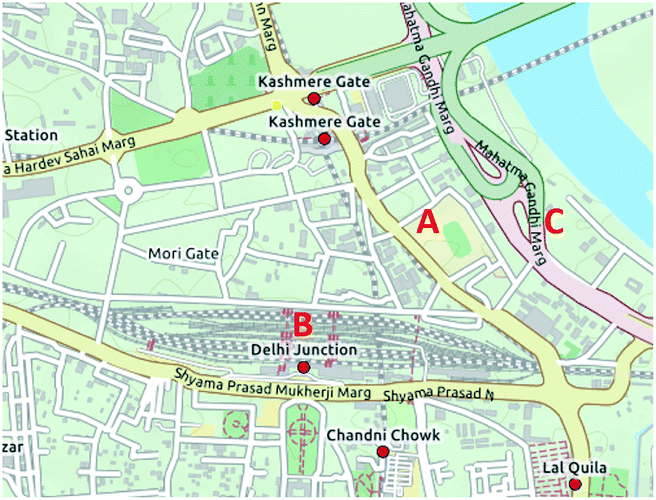 | ||
| Fig. 1 Map of (A) IGDTUW, (B) Old Delhi railway junction and (C) National Highway 44. © OpenStreetMap contributors. | ||
Gas chromatography
The DC-GC-FID made measurements from 28-May to 05-Jun 2018 and 5 to 27-Oct 2018, with 31 C2–C7 NMHCs and C2–C5 oxygenated volatile organic compounds measured.45 A 500 ml sample (1.5 L pre-purge of 100 ml min−1 for 15 min, sample at 25 ml min−1 for 20 min) was collected (Markes International CIA Advantage), passed through a glass finger at −30 °C to remove water and adsorbed onto a dual-bed sorbent trap (Markes International ozone precursors trap) at −20 °C (Markes International Unity 2). The sample was thermally desorbed (250 °C for 3 min) in a flow of helium carrier gas then split 50:50 and injected into two separate columns for analysis of NMHCs (50 m × 0.53 mm Al2O3 PLOT) and oxygenated volatile organic compounds (10 m × 0.53 mm LOWOX with 50 μm restrictor to balance flow). The oven was held at 40 °C for 3 min, then heated at 12 °C min−1 to 110 °C and finally heated at 7 °C min−1 to 200 °C with a hold of 20 min.
The GC×GC-FID made measurements from 29-May to 05-Jun 2018 and 11-Oct to 04-Nov 2018. It was used to measure 64 C7–C12 hydrocarbons (alkanes, monoterpenes and monoaromatics). The mean, minimum and maximum mixing ratios measured using both GCs from both campaigns are summarised in the ESI2.† The GC×GC-FID collected 2.1 L samples (70 ml min−1 for 30 min) using an adsorption-thermal desorption system (Markes International Unity 2). NMHCs were trapped onto a sorbent (Markes International U-T15ATA-2S) at −20 °C with water removed in a glass cold finger (−30 °C). The sample was thermally desorbed (250 °C for 5 min) and injected splitless down a transfer line. It was refocussed for 60 s using liquid CO2 at the head of a non-polar BPX5 held at 50 psi (SGE Analytical 15 m × 0.15 μm × 0.25 mm) which was connected to a polar BPX50 at 23 psi (SGE Analytical 2 m × 0.25 μm × 0.25 mm) via a modulator held at 180 °C (5 s modulation, Analytical Flow Products MDVG-HT). The oven was held for 2 min at 35 °C, then ramped at 2.5 °C min−1 to 130 °C and held for 1 min with a final ramp of 10 °C min−1 to 180 °C and hold of 8 min. Both GC systems were tested for breakthrough to ensure trapping of the most volatile components (see the ESI3†). Calibration was carried out using a 4 ppbv gas standard containing a range of NMHCs from the British National Physical Laboratory (NPL, UK). The linearity of the detector response at higher mixing ratios was confirmed post-campaign by carrying out a calibration using multiple injections at a range of mixing ratios of benzene up to 3 times greater than the maximum observed ambient mixing ratio (see the ESI4†). NMHCs not in the gas standard were quantified using the relative response of liquid standard injections to toluene, as detailed in the ESI5.† This included quantification and qualification of 12 monoterpenes, tentative identification of C4 substituted monoaromatics (see the ESI6†) and quantification of C12–C14 alkanes. The inlet used by both instruments was located approximately 5 m above the ground with sample lines run down 1/2′′ PFA tubing to the laboratory.
Supporting measurements
Nitrogen oxides (NOx = NO + NO2) were measured using a dual-channel chemiluminescence instrument (Air Quality Designs Inc., Colorado). Carbon monoxide (CO) was measured using a resonance fluorescence instrument (Model AL5002, Aerolaser GmbH, Germany). Ozone measurements were made using a 49i (Thermo Scientific) with a limit of detection of 1 ppbv. The CO and NOx instruments were calibrated regularly (every 2–3 days) throughout both campaigns using standards from the NPL, UK. The setup and calibration procedures were identical to those described by Squires et al. (2020).46PTR-QiTOF-MS (Ionicon Analytik, Innsbruck) measurements were made from 26/05/2018 to 09/06/2018 in the pre-monsoon campaign and from 04/10/2018 to 23/11/2018 in the post-monsoon campaign. For the pre-monsoon and post-monsoon campaign up until 05/11/2018, the sample inlet was positioned 5 m above the ground adjacent to the inlet used for GC measurements. The PTR-QiTOF-MS subsampled from a 1/2′′ PFA common inlet line running from this inlet to an air-conditioned laboratory where the instrument was installed with a flow of around 20 L min−1. From 05/11/2018 to 23/11/2018 the inlet was moved to a flux tower approximately 30 m above ground level. The PTR-QiTOF-MS was operated with a drift pressure of 3.5 mbar and a drift temperature of 60 °C giving an E/N (the ratio between electric field strength and buffer gas density in the drift tube) of 120 Td.
The PTR-QiTOF-MS was calibrated daily using a 19 component 1 ppmv gas standard (Apel Riemer, Miami) dynamically diluted into zero air to provide a 3-point calibration. Volatile organic compounds were then quantified using a transmission curve.47 Mass spectral analysis was performed using PTRwid.48 A comparison of toluene measured by PTR-QiTOF-MS and GC×GC-FID is presented in the ESI7.†
Windspeed and direction were taken from measurements at Indira Gandhi International Airport in 2018, approximately 16 km southwest of the site. Modelled Planetary Boundary Layer Height (PBLH) data was downloaded (Lat. 28.625, Lon. 77.25) from the fifth-generation reanalysis (ERA5) from the European Centre for Medium-Range Weather Forecasts at 0.25 degree resolution with a 1 hour temporal resolution.49
Receptor models
The mixing ratio of NMHC i in the kth sample, Cik, can be described by eqn (1):50 | (1) |
Principle component analysis (PCA) is a type of factor analysis which has been used to decompose many different NMHCs measured into a set of factors which are used to represent their sources.50–54 It is appropriate to use with datasets with only a few underlying factors. Principal component analysis has been performed in R on the data collected in this study, retaining the 4 factors with eigen values >1.52 This process is well described elsewhere.50
The contribution of each source was determined by absolute principle component scores (APCS).53–55 The first step involves normalisation of NMHC, Zik:
 | (2) |
 | (3) |
The source contributions are determined by eqn (4):
 | (4) |
 is determined by subtracting the factor scores from the true sample in eqn (2) from those obtained in eqn (3),54bki = coefficient of regression for source k for NMHC i54 and p = number of sources. The product
  shows the contribution to the airborne mixing ratio of NMHC i from source p. Eqn (4) is solved through multiple linear regression analysis. Due to the potentially colinear nature of many diurnal profiles in Delhi, factors with small non-meaningful contributions to chemical species (<20%) have been deemed to be insignificant and filtered out from the analysis. Furfural, measured by PTR-QiTOF-MS, has been included as a tracer for burning emissions to help with the identification of factors.28,57,60 The result from PCA/APCS has been compared to those calculated using the EPA Unmix 6.0 source apportionment toolkit,58 which has been previously applied to many air quality datasets.59 The use of multiple source apportionment methods should result in a more robust conclusion.
Results and discussion
Meteorological overview
Fig. 2 shows seasonal wind rose plots for windspeed and direction measured at Indira Gandhi International Airport in 2018, downloaded from the Integrated Surface Database provided by the National Oceanic and Atmospheric Administration (NOAA).60,61 Air masses predominantly approached Delhi from the west/north west in winter and spring. During the pre-/post-monsoon and monsoon seasons, air masses generally approached from either the west/north west or east/south east. Conditions were most stagnant in the winter and post-monsoon seasons with the lowest windspeeds (averages of 1.8 and 1.9 m s−1, respectively) and the largest percent of calm periods, where the wind speed was below <0.5 m s−1 (25.7–28.0%). Windspeeds were higher in spring, pre-monsoon and monsoon seasons (with averages in the range 2.6 to 3.3 m s−1, respectively), with the lowest amount of calm periods in the pre-monsoon and monsoon seasons (6.4 and 7.5%, respectively) (see the ESI8† for monthly analysis). | ||
| Fig. 2 Seasonal wind rose plots at Indira Gandhi International Airport in 2018. | ||
The lowest windspeeds were at night during the post-monsoon and winter seasons, with a mean windspeed of <1 m s−1. The PBLH was highest at night during the pre-monsoon and monsoon seasons at around 160–200 m and lowest during winter, spring and post-monsoon seasons at around 55–85 m. The mean PBLH was highest in the pre-monsoon season at approximately 2450 m, when temperatures peaked at 45–50 °C. The mean daytime PBLH was similar in post-monsoon and spring seasons at around 1400–1500 m and monsoon/winter seasons at around 1030 m (seasonal mean diurnal profiles of windspeed and PBLH are provided in the ESI9†).
Fig. 3 shows 10 m 96 h NOAA HYSPLIT (Hybrid Single Particle Lagrangian Integrated Trajectory) back trajectories clustered (Angle) from pre- and post-monsoon campaigns with mean toluene mixing ratio coloured by cluster.60 Back trajectories in the pre-monsoon campaign were generally long (C2–C4 at around 1000 km over 96 h), suggesting higher windspeeds with monsoon-type wind patterns, and resulted in low toluene mixing ratios. C1 was important from 27–29/05/18 and followed a much shorter trajectory and resulted in higher toluene mixing ratios, highlighting the impact of shorter, slower moving trajectories in allowing the build-up of local pollution. Trajectories in the post-monsoon campaign were generally shorter, and toluene mixing ratios higher.
 | ||
| Fig. 3 Clustered NOAA Hysplit back trajectories from pre- and post-monsoon campaigns (left) and mean toluene mixing ratios by cluster (right). | ||
NMHC mixing ratios and diurnal cycles
Hourly measurements of 90 individual NMHCs were obtained from both GC instruments over the two campaigns. Relatively high mixing ratios of NMHCs were observed during both campaigns, but with significant enhancements observed from 17/10/2018 until the end of the post-monsoon measurement period on the 27/10/2018. Fig. 4A and C show stacked area plots of NMHC mixing ratios during pre- and post-monsoon campaigns. NMHC concentrations in the pre-monsoon campaign were generally much lower, except for two large alkane spikes caused by very large concentrations of propane and butane (Fig. 4A). In the post-monsoon campaign, NMHC concentrations at night were significantly larger than in the pre-monsoon campaign. Fig. 4B and D show concentration–time series of O3, CO and NOx from pre- and post-monsoon campaigns. Significant night-time enhancement of CO and NOx was observed in the post-monsoon. O3 peaked in the pre-monsoon at around 80–90 ppbv and around 60–90 ppbv in the post-monsoon. | ||
| Fig. 4 Concentration–time series of (A) pre-monsoon NMHCs (stacked), (B) pre-monsoon O3, NO, NO2 and CO, (C) post-monsoon NMHCs (stacked) and (D) post-monsoon O3, NO, NO2 and CO. Zoomed in versions for the pre-monsoon campaign are available in the ESI10.† | ||
Fig. 5 shows the mean diurnal profiles using data combined from both campaigns for propane (A), n-hexane (B), isoprene (C), toluene (D), n-tridecane (E) and ethanol (F). These have been chosen as they are typical NMHC tracers from different sources. Diurnal profiles of individual data from the pre- and post-monsoon campaigns are given in the ESI11.† The diurnal profiles observed for propane, n-hexane, toluene and n-tridecane were similar, peaking at night between 8 pm and 6 am with a minimum in the afternoon. For propane, large spikes were present around midday, with the spikes present but less pronounced in the post-monsoon campaign. These large increases in mixing ratios have been attributed to emissions from LPG, a mixture of propane and butane, from lunchtime cooking activities. The average diurnal profile for n-hexane during the pre-monsoon (see the ESI11†) showed a small peak around lunchtime likely from midday traffic. A small peak was present for toluene from 8–10 am, potentially from the morning rush hour before the boundary layer begins to expand. Isoprene showed a typically distinct biogenic diurnal profile and peaked around midday. However, mixing ratios remained high at night (around 0.5 ppbv), possibly indicating an additional anthropogenic source which may be automotive or burning related.62–65 For example, Stewart et al. (2020) showed that combustion of municipal solid waste, cow dung cake and sawdust collected from Delhi could lead to emission of anthropogenic isoprene.28 A pronounced diurnal profile was present for n-tridecane which was highest at night, potentially amplified by night-time residential generator usage and restrictions which allow the entry of heavy goods vehicles to the city only at night. A peak was present for ethanol around midday, which was most pronounced in the pre-monsoon campaign and may be from increased volatilization due to increased temperature and radiation.
 | ||
| Fig. 5 Diurnal profiles of selected NMHCs from pre- and post-monsoon campaigns for (a) propane, (b) n-hexane, (c) isoprene, (d) toluene, (e) n-tridecane and (f) ethanol. The shaded region indicates the 95% confidence interval in the means. | ||
In order to compare the composition of NMHCs during the two campaigns, average diurnal profiles were calculated for all NMHC during the two campaigns and split according to functionality (alkanes, aromatic, monoterpenes). Fig. 6A and B show the average diurnal profiles for all alkanes. During the pre-monsoon campaign, the largest alkane mixing ratios were from 10:00–14:00 and caused by very large mixing ratios of propane and butane, with the mean for both campaigns peaking at around 150 ppbv. Outside of these peaks, the highest mixing ratios were observed at 20:00 at approximately 50 ppbv. The lowest mixing ratios of 20 ppbv were observed at 04:00. In the post-monsoon campaign, mixing ratios were high from 20:00–08:00 and peaked at around 360 ppbv at 21:00. Fig. 6C and D show the average diurnal profiles for aromatic species from the pre- and post-monsoon campaigns. Both campaigns showed peaks likely from traffic between 08:00–12:00. During the pre-monsoon, mixing ratios peaked at 19 ppbv at 19:00 and reduced to around 5 ppbv at midnight and remained low until the rush hour. In the post-monsoon, the mean diurnal variation of aromatic mixing ratios peaked at 96 ppbv at 21:00. The mixing ratio at 12:00 in the post-monsoon campaign was around 3 times larger (14 ppbv) than at the same time in the pre-monsoon average diurnal profile (5 ppbv). The lowest mixing ratios observed in the pre-monsoon campaign were at 15:00 (4.2 ppbv) and at 14:00 in the post-monsoon campaign (8.8 ppbv). Fig. 6E shows that in the average diurnal profile during the pre-monsoon the monoterpenes peaked at 07:00 (0.19 ppbv) and 22:00 (0.18 ppbv), likely due to biogenic emissions before the effect of photochemical degradation was too pronounced. Post-monsoon monoterpenes (Fig. 6F) peaked from 22:00–07:00. The largest contributors to post-monsoon mixing ratios were limonene (31%) and β-ocimene (25%). The contribution of β-ocimene was similar in the pre-monsoon, with a lower contribution of limonene (8%) and larger contributions of α-pinene (28%), α-phellandrene (14%) and 3-carene (12%). The lowest monoterpene mixing ratios observed were in the afternoon at similar mixing ratios in the pre- (0.07 ppbv) and post-monsoon periods (0.09 ppbv), with a minimum at 15:00. The diurnal profile of the monoterpenes in the post-monsoon period was very similar to the anthropogenic NMHCs, with high concentrations of very reactive monoterpenes observed. In the time series in Fig. 4C, up to 6 ppbv of monoterpenes were measured. Comparably high unspeciated mixing ratios of monoterpenes have been previously reported in India.66
 | ||
| Fig. 6 Stacked average diurnal profiles of alkanes (A and B), aromatics (C and D) and monoterpenes (E and F) measured during the pre- and post-monsoon campaigns in Delhi in 2018. Zoomed in stacked diurnals from the pre-monsoon campaign are given in the ESI12.† | ||
Fig. 7A and B show the diurnal variation of the toluene mixing ratio, PBLH and windspeed during the pre- and post-monsoon campaigns. The shape of the toluene diurnal was similar in both campaigns, but the mixing ratio of toluene much larger in the post-monsoon campaign. The windspeed in the pre-monsoon campaign (3–4 m s−1) was consistent throughout the day and the night-time PBLH was around 300 m. In the post monsoon both night-time windspeed (∼0.9 m s−1) and PBLH (∼60 m) were lower, resulting in higher toluene mixing ratios.
 | ||
| Fig. 7 Variation of toluene mixing ratio, PBLH and windspeed in (A) pre-monsoon campaign from 26/05/18–09/06/18 and (B) post-monsoon campaign from 06/10/18–23/11/18. Mean diurnal profiles of O3, NO, NO2 and CO in (C) pre- and (D) post-monsoon campaigns. Error bars represent the 95% confidence intervals in the mean. (A) averaged over the same sample period as (C), is given in the ESI13.† Polar plots of (E) toluene from 26/05/18–09/06/18 and 06/10/18–23/11/18 and (F) CO from 28/05/18–05/06/18 and 07/10/18–23/11/18, with the radial component reflecting wind speed in m s−1.60 | ||
Fig. 7C and D show the average diurnal profiles of the O3, NO, NO2 and CO measured during the pre- and post-monsoon campaigns. In the pre-monsoon campaign, mean O3 peaked at 14:00 (90 ppbv) and remained high from 20:00–08:00 at ∼30 ppbv. Average mixing ratios of NO (24–55 ppbv) and CO (0.67–1.3 ppmv) were elevated at night, with NO reducing to ∼1.3 ppbv from 14:00–15:00 and CO to 0.4–0.5 ppmv from 12:00–16:00. In the post-monsoon campaign mean O3 was low (<5 ppbv) from 18:00–08:00 and peaked at 81 ppbv at 13:00. Night-time mixing ratios of NO (around 200 ppbv) and CO (approximately 2–3 ppmv) remained high from around 20:00–08:00. NO2 showed less variability, with a mean mixing ratio of ∼40 ppbv from 00:00–08:00 with two peaks at 09:00 (55 ppbv) and 17:00 (65 ppbv). There was a clear enhancement of primary pollutants NO, CO and NMHCs in Delhi during the post-monsoon at night, which appears to be driven, at least in part, by a very shallow and stagnant boundary layer.
A bivariate polar plot of the toluene concentration measured using PTR-QiTOF-MS during pre- (26/05/18–09/06/18) and post-monsoon (07/10/18–23/11/18) seasons is shown in Fig. 7E and for CO in pre- (28/05/18–05/06/18) and post-monsoon (07/10/18–23/11/18) campaigns in Fig. 7F. Most of the NMHCs presented in this paper show a similar trend, with the highest mixing ratios observed under low windspeeds and PBLH indicating they are likely the result of emissions from the local area, perhaps with a larger source directly to the East.
Regression analysis
In order to determine the relative source strength of different NMHCs a number of different regression techniques were used. The observed mixing ratios of NMHCs were plotted against the mean CO and acetylene (tracers for petrol vehicles) measured during the concurrent GC sample time, with the regression coefficient of determination, R2, examined. Fig. 8 shows the observed R2 values for different carbon numbers with the points coloured by functionality. Shaded regions have been added to group NMHCs that were indicative of major emission sources. C3–C4 alkanes, normally attributed to LPG emissions,67,68 were grouped together, with low R2 values in the pre-monsoon campaign (<0.4) and shaded in red. The low R2 value to CO indicated that these likely were fugitive emissions from LPG rather than combustion. Removal of the few measurement points which caused the large peaks in propane and butane, shown as large spikes in alkanes between 11:00–13:00 in Fig. 6A, confirmed this and remaining measurements had much higher R2 to CO and acetylene (shown as red shaded area with red dashed line). C5–C10 alkanes, as well as some C4 alkenes (green shading), were grouped with R2 values ∼0.7–0.9 and may be from a petrol source as CO is a conventional tracer for petrol vehicular exhaust emissions. The R2 value then decreased for C10–C15 alkanes, which could be indicative of a different source (blue shading), with a poorer relationship to CO such as diesel or burning. Aromatic species are located in the regions characteristic of petrol and diesel emissions, and isomers with C10 showed the greatest variability spanning a range of R2 values with CO from 0.1–0.9. Monoterpenes were also placed onto Fig. 8 and a range of R2 values were observed, possibly indicating a range of sources for these species. The overall shape between the two campaigns appeared similar, however, the R2 values for the post-monsoon campaign were greater, and may be driven by strong meteorological influences, higher levels of pollution and reduced photochemistry. The monoterpenes in particular showed a much stronger correlation with CO during the post-monsoon period suggesting an anthropogenicsource. This may potentially be from sources such as combustion, cooking spices or personal care products.29,56,69,80,81 This conclusion is similar to that reported by Wang et al. (2020) who suggested that biogenic molecules may be explained by vehicular or burning sources in Delhi.42 | ||
| Fig. 8 R 2 as a function of carbon number from regression analysis of NMHCs against CO and acetylene during pre- and post-monsoon campaigns. See text for discussion of the shaded ellipses. | ||
Fig. 9 shows the R2 of linear regression plots of different NMHCs measured during pre- and post-monsoon campaigns ordered according to hierarchical cluster analysis, created with data extracted from the corPlot function of openair.60 A region is marked with a red dashed line which contained two closely correlated regions with NMHCs characteristic of diesel (blue) and petrol (green) fuels. There was likely some crossover of C8–C10 species in this region, owing to similar diurnal profiles of NMHCs characteristic of petrol/diesel emissions. Benzene and toluene also sat with the diesel region but were likely to come from both vehicular sources, and toluene showed a stronger correlation with C4–C6 tracers than benzene. A further region with propane and butane (white square) was identified and characteristic of emissions from LPG fuels. Acetone and methanol were poorly correlated to other NMHCs, indicating a different source, which was assumed to be secondary chemistry or volatilisation for methanol. Isoprene was poorly correlated to other NMHCs, with an assumed daytime biogenic source due to the diurnal profile in Fig. 5C. A further small region was identified (orange square) containing C11–C14 aliphatic species, which were tentatively identified as coming from a mixture of diesel/burning sources. These species showed strong correlations to each other but poorer correlation with other NMHCs.
 | ||
| Fig. 9 Correlation and hierarchical cluster analysis of NMHC mixing ratios using a combined dataset from both pre- and post-monsoon campaigns. Light blue shaded region corresponds to hydrocarbons typically associated with diesel fuel, green region to petrol, white region to LPG and orange region to diesel/burning. | ||
Emission ratio evaluation
The ratio of specific NMHC tracer pairs in ambient samples can be indicative of their emission source(s). The atmospheric lifetimes of i-pentane and n-pentane are similar;70 a concentration ratio of 0.8–0.9 is typically observed for natural gas drilling, 2.2–3.8 for vehicular emissions, 1.8–4.6 for evaporative fuel emissions and 0.5–1.5 for biomass burning.29,71Fig. 10 shows the i-pentane to n-pentane ratio measured in this study, which was found to be 2.6. This was compared to vehicular exhaust emissions reported from the Pearl River Tunnel in Guangzhou, China, where the ratio was found to be 2.9.72 The ratio measured in Delhi was also similar to another site considered to be highly influenced by traffic related emissions (Jingkai community, Zhengzhou, Henan Province, China in 2017) which also showed a ratio of 2.6.71 The high R2 of 0.98 in the Delhi measurements indicated a constant pollution source (mix), with a ratio close to that characteristic of vehicular emissions.
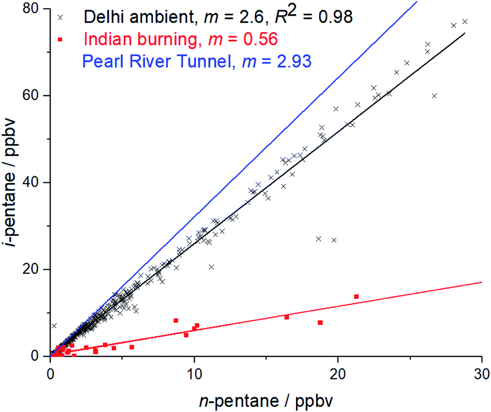 | ||
| Fig. 10 Comparison of i/n-pentane ratios between Delhi (black), Indian solid fuel combustion (red)29 and the Pearl River Tunnel China (blue).72 | ||
The ratio of benzene to toluene in ambient samples has also been compared to those from different sources. During the post-monsoon campaign, the mean benzene/toluene ratio was 0.36. This has been compared to the ratios measured from the headspace of petrol (0.4) and diesel (0.2) liquid fuel samples collected from Delhi29 and that of 0.3 reported for traffic exhaust emissions.73 Whilst there is uncertainty in the exact ratio of benzene/toluene at emission due to the increased reactivity of toluene relative to benzene, the presence of a significantly greater molar ratio of toluene to benzene in ambient samples underlines the importance of petrol and diesel emissions to NMHCs in Delhi, as this could not be explained by solid fuel combustion sources for which benzene/toluene ratios have been reported for wood (2.3) and cow dung cake (0.9).29
Source apportionment modelling
Fig. 11 shows the mean contribution of the 4 factors selected to pollutant mixing ratios from the PCA/APCS model. The PCA/APCS model was initially run with 3–7 factors, however, inclusion of >4 factors did not lead to a significantly improved output and running EPA Unmix 6.0 with >4 factors often led to solutions which would not converge. Sources in this study have been attributed to factors according to the species which they predict and those suggested in previous studies which showed emissions of C2–C5 for natural gas, C2–C10 for petrol and diesel emissions >C8.74 The LPG factor in this study contributed to C3–C4 hydrocarbons. The petrol factor contributed to C2–C12 hydrocarbons and contributed significantly to alkanes from C5–C9. The petrol factor had a smaller contribution to C11–C12 hydrocarbons and was probably due to slight collinearity of petrol and diesel factors due to similar diurnal profiles and strong meteorological influences. The diesel factor increased in importance from C8–C14 NMHCs, as expected of a diesel source. The inclusion of a small number of factors was beneficial to factor identification in this study, as the diurnal profiles of all NMHCs in the post monsoon were very similar. It was not possible to resolve a second diesel factor which could be explained by diesel emissions from vehicles and generators. The assignment of petrol and diesel factors compared well with previous studies which showed that aromatics and alkanes were the dominant emission from 4-stroke motorcycles, light petrol vehicles and diesel trucks.75–77 The burning factor was rationalised using furfural as a tracer and contributed to C2–C7 hydrocarbons and >C12 hydrocarbons. North Indian burning sources have been shown to release substantial amounts of furfural and had significant emission factors of smaller alkanes such as ethane and open burning of municipal solid waste has been shown to contribute to emissions of heavier alkanes.28,29 Previous studies have also reported emissions of n-alkanes from the burning of municipal solid waste.78 It is noteworthy that very low mean mixing ratios of furfural (0.8 ppbv) were measured by PTR-QiTOF-MS in the post-monsoon campaign compared to other NMHCs such as monoterpenes (1.3 ppbv) and toluene (18 ppbv), which is suggestive of a small burning source. | ||
| Fig. 11 Mean contribution of sources to NMHCs measured in Delhi by PCA/APCS. Unmix 6.0 outputs are given in the ESI14.† | ||
Table 1 shows the estimated source contributions to mean mixing ratio (M.R) and mass observed in ambient samples predicted by PCA/APCS and the EPA Unmix 6.0 toolkit. This study showed that traffic related emissions, which also included some emissions from static diesel generators, were the dominant source of NMHCs at the site, with relative mean mixing ratio contributions predicted by the PCA/APCS and Unmix models from petrol automobiles and motorbikes (38%), diesel trucks, trains and generators (14%), LPG from cooking and vehicles (32%) and open burning of biomass and municipal solid waste (16%). The mean mass contributions were petrol (39%), diesel (23%), LPG (24%) and burning (14%). High mixing ratios of aromatics were dominated by traffic related sources and meant that the contribution of biomass burning to these was insignificant.
| Method | By | LPG | Burning | Petrol | Diesel |
|---|---|---|---|---|---|
| PCA/APCS | M.R | 30 | 15 | 44 | 11 |
| EPA Unmix 6.0 | M.R | 34 | 18 | 32 | 16 |
| PCA/APCS | Mass | 23 | 10 | 47 | 20 |
| EPA Unmix 6.0 | Mass | 25 | 18 | 30 | 27 |
This study compared well to the limited previous literature focussed on NMHC source apportionment in Delhi from ambient measurements42 and inventories which have shown the importance of vehicular emissions.15,25,26 Gujar et al. (2004) showed that from 1990–2000 transport represented >80% of NMHC emissions, with 47% of emissions from motorcycles25 and the study led by NEERI in 2008 showed vehicular related emissions to be the largest citywide source.39 Petrol emissions were the largest source shown by Srivastava et al. (2009)41 and the inventory for India produced by Sharma et al. (2015)15 commented that large built up areas like Delhi were dominated by petrol traffic related emissions. The most recent study led by Wang et al. (2020) determined that traffic was responsible for 57% of the mixing ratio of NMHCs at an urban site in Delhi, with 16% from secondary sources and 27% from biomass burning.42 The larger contribution of traffic related emissions and lower contribution of burning emissions in this present study were explained by the proximity of major roads to the IGDTUW site. It was also explained by the fact that the GC instrumentation used in this study was specifically targeted to NMHCs, in comparison to PTR-TOF-MS which is more suited to measuring oxygenated species commonly from secondary sources and burning. The contribution by mass of petrol and diesel sources in this study (62%) is in good agreement with that suggested by a 1 km2 gridded inventory of Delhi (65%).26
The results of the PCA/APCS and Unmix 6.0 models were compared to 3–6 factor unconstrained solutions from EPA PMF 5.0 run on individual pre-/post-monsoon datasets as well as the combined dataset. Although PMF is widely accepted as a more powerful receptor model due to being able to find more factors, PMF explored variance within the petrol and diesel factors before finding the factor attributed to LPG (see the ESI15† for comparison of the 4-factor solution using the combined dataset). The instrumental uncertainty in the large fugitive spikes in propane and butane was not large, and so these points had not been down weighted within the model for this reason. Inclusion of benzene/toluene ratios and propane/butane ratios of factors in the PMF model did not lead to a significantly improved result and PMF was only able to identify the LPG factor in the 6-factor pre-monsoon dataset. Factor identification for model runs with inclusion of additional factors was increasingly difficult to interpret. This may be partly driven by the limited data collected during the short measurement periods of this study. For these reasons, the results from the PMF model were not included in this study. Whilst studies criticise source apportionment in India using PCA/APCS and Unmix,79 the results of the PCA/APCS and Unmix models were considered beneficial to include as they agreed with other source apportionment analyses and compared well to literature.
This study only focussed on the major sources of NMHCs in Delhi. It is expected that any CNG transport related emissions which may be >C1, potentially from poor maintenance and lubricant emissions, are grouped with petrol emissions. This study does not account for smaller sources such as emissions from industry, powerplants and brick kilns. The contribution of LPG emissions from cooking and vehicles was larger than estimated in current inventories.
Conclusion
This study presented a comprehensive suite of NMHC measurements performed at an urban site in Delhi during the pre- and post-monsoon seasons in 2018. Extremely high night-time mixing ratios were measured during the post-monsoon campaign, caused by stagnant conditions and a shallow boundary layer. A range of source apportionment techniques were used, which appear self-consistent and arrived at similar conclusions for correlation analysis to CO, acetylene and other NMHCs as well as hierarchical cluster analysis. The absolute contributions of different sources were determined through receptor models, with factors rationalised using recent studies focused on emissions from petrol, diesel and solid fuel combustion sources and confirmed through comparison of characteristic i-/n-pentane and benzene/toluene ratios which were close to those of liquid automotive fuels. These results were in line with bottom-up emissions inventory and top-down receptor modelling approaches from recent literature. Unusually high levels of very reactive monoterpenes were observed at night during the post-monsoon campaign, with similar diurnal profiles to NMHCs typical of petrol and diesel sources. This suggested that these species were emitted from anthropogenic sources in Delhi rather than the conventional biogenic source seen in other locations. The impact of prolonged exposure to elevated NMHC concentrations at night during the post-monsoon campaign is likely to lead to significant health impacts and result in the production of high levels of other harmful secondary pollutants, when photochemical oxidation can occur the following day. In order to reduce the high levels of pollutants during the post-monsoon period, policies that target vehicle emission reductions are critical.Author contributions
GJS made measurements with GC×GC-FID, conducted source analysis and led the paper. BSN/JRH setup, made measurements and processed the data for the DC-GC-FID. WJFA and BL made measurements of NMHCs by PTR-QiTOF-MS, supported by CNH. ARV/WSD made measurements of CO, NO, NO2 and O3. RED made measurements with GC×GC-FID. EN/NM/S/RG assisted with logistics of lab setup and data analysis. ERV assisted with interpretation of meteorological parameters. ARR/JDL/JFH provided overall guidance with setup, conducting and running of instruments and interpreting and analysing data. All authors assisted with lab setup, logistics, data analysis as well as the discussion, writing and editing of the manuscript.Conflicts of interest
The authors declare that they have no conflict of interest.Acknowledgements
This work was supported by the Newton-Bhabha fund administered by the UK Natural Environment Research Council, through the DelhiFlux project of the Atmospheric Pollution and Human Health in an Indian Megacity (APHH-India) programme (grant reference NE/P016502/1). GJS, BSN and WSD acknowledge the NERC SPHERES doctoral training programme for studentships. The authors thank the National Centre for Atmospheric Science for providing the DC-GC-FID instrument. The meteorological data in this study was taken from National Oceanic and Atmospheric Administration.References
- UN, in World Urbanisation Prospects, UN, New York, USA, 2014, ch. 1, p. 1 Search PubMed.
- World Health Organisation, Burden of disease from ambient air pollution for 2016, WHO, Geneva: Switzerland, 2018 Search PubMed.
- J. Huff, Int. J. Occup. Environ. Health, 2007, 13, 213–221 CrossRef CAS PubMed.
- D. H. Ehhalt, in Global Aspects of Atmospheric Chemistry, ed. R. Zellner and H. Steinkopff, Germany, 1999, ch. 2.1, pp. 21–24 Search PubMed.
- F. Dentener, R. Derwent, E. Dlugokencky, E. Holland, I. Isaksen, J. Katima, V. Kirchhoff, P. Matson, P. Midgley and M. Wang, in IPCC Third Assessment Report: Climate Change 2001 (TAR). Working Group I: The Scientific Basis, ed. F. Joos and M. McFarlan, Intergovernmental Panel on Climate Change, Geneva, Switzerland, 2001, ch. 4.2.3.2, pp. 241–287 Search PubMed.
- K. Sindelarova, C. Granier, I. Bouarar, A. Guenther, S. Tilmes, T. Stavrakou, J. F. Müller, U. Kuhn, P. Stefani and W. Knorr, Atmos. Chem. Phys., 2014, 14, 9317–9341 CrossRef.
- J. F. Lamarque, T. C. Bond, V. Eyring, C. Granier, A. Heil, Z. Klimont, D. Lee, C. Liousse, A. Mieville, B. Owen, M. G. Schultz, D. Shindell, S. J. Smith, E. Stehfest, J. Van Aardenne, O. R. Cooper, M. Kainuma, N. Mahowald, J. R. McConnell, V. Naik, K. Riahi and D. P. van Vuuren, Atmos. Chem. Phys., 2010, 10, 7017–7039 CrossRef CAS.
- G. Huang, R. Brook, M. Crippa, G. Janssens-Maenhout, C. Schieberle, C. Dore, D. Guizzardi, M. Muntean, E. Schaaf and R. Friedrich, Atmos. Chem. Phys., 2017, 17, 7683–7701 CrossRef CAS.
- J. Kurokawa, T. Ohara, T. Morikawa, S. Hanayama, G. Janssens-Maenhout, T. Fukui, K. Kawashima and H. Akimoto, Atmos. Chem. Phys., 2013, 13, 11019–11058 CrossRef CAS.
- J. Kurokawa and T. Ohara, Atmos. Chem. Phys. Discuss., 2019, 2019, 1–51 Search PubMed.
- C. K. Varshney and P. K. Padhy, J. Ind. Ecol., 1998, 2, 93–105 CrossRef CAS.
- D. G. Streets, T. C. Bond, G. R. Carmichael, S. D. Fernandes, Q. Fu, D. He, Z. Klimont, S. M. Nelson, N. Y. Tsai, M. Q. Wang, J. H. Woo and K. F. Yarber, J. Geophys. Res. Atmos., 2003, 108, 8809 CrossRef.
- T. Ohara, H. Akimoto, J. Kurokawa, N. Horii, K. Yamaji, X. Yan and T. Hayasaka, Atmos. Chem. Phys., 2007, 7, 4419–4444 CrossRef CAS.
- Q. Zhang, D. G. Streets, G. R. Carmichael, K. B. He, H. Huo, A. Kannari, Z. Klimont, I. S. Park, S. Reddy, J. S. Fu, D. Chen, L. Duan, Y. Lei, L. T. Wang and Z. L. Yao, Atmos. Chem. Phys., 2009, 9, 5131–5153 CrossRef CAS.
- S. Sharma, A. Goel, D. Gupta, A. Kumar, A. Mishra, S. Kundu, S. Chatani and Z. Klimont, Atmos. Environ., 2015, 102, 209–219 CrossRef CAS.
- United Nations, World Urbanization Prospects: The 2018 Revision (ST/ESA/SER.A/420), United Nations: Department of Economic and Social Affairs, Population Division, New York, 2019 Search PubMed.
- WHO, Ambient (outdoor) air pollution in cities database 2014, World Health Organization, Geneva, Switzerland, 2014 Search PubMed.
- P. Kumar, S. Jain, B. R. Gurjar, P. Sharma, M. Khare, L. Morawska and R. Britter, Atmos. Environ., 2013, 71, 198–201 CrossRef CAS.
- P. Kumar, M. Khare, R. M. Harrison, W. J. Bloss, A. C. Lewis, H. Coe and L. Morawska, Atmos. Environ., 2015, 122, 657–661 CrossRef CAS.
- S. Gani, S. Bhandari, S. Seraj, D. S. Wang, K. Patel, P. Soni, Z. Arub, G. Habib, L. Hildebrandt Ruiz and J. S. Apte, Atmos. Chem. Phys., 2019, 19, 6843–6859 CrossRef CAS.
- E. Reyes-Villegas, U. Panda, E. Darbyshire, J. Cash, R. Joshi, B. Langford, C. F. Di Marco, N. Mullinger, J. Acton, W. Drysdale, E. Nemitz, M. Flynn, A. Voliotis, G. McFiggans, H. Coe, J. Lee, C. N. Hewitt, M. R. Heal, S. S. Gunthe, S. Shivani, R. Gadi, S. Singh, V. Soni and J. Allan, Atmos. Chem. Phys. Discuss., 2020 DOI:10.5194/acp-2020-894.
- J. Cash, B. Langford, C. Di Marco, N. Mullinger, J. D. Allan, E. Reyes-Vellegas, R. Joshi, M. Heal, W. J. Acton, W. Drysdale, T. Mandal, Shivani, R. Gadi and E. Nemitz, Atmos. Chem. Phys. Discuss., 2020 DOI:10.5194/acp-2020-1009.
- Y. Chen, Atmos. Chem. Phys. Discuss., 2020 10.1039/D0FD00087F.
- R. K. Bose and G. Anandalingam, Energy, 1996, 21, 305–318 CrossRef CAS.
- B. R. Gurjar, J. A. van Aardenne, J. Lelieveld and M. Mohan, Atmos. Environ., 2004, 38, 5663–5681 CrossRef CAS.
- S. K. Guttikunda and G. Calori, Atmos. Environ., 2013, 67, 101–111 CrossRef CAS.
- R. Goel and S. K. Guttikunda, Atmos. Environ., 2015, 105, 78–90 CrossRef CAS.
- G. J. Stewart, B. S. Nelson, W. J. F. Acton, A. R. Vaughan, N. J. Farren, J. R. W. Hopkins, M. Ward, S. J. Swift, R. Arya, A. Mondal, R. Jangirh, S. Ahlawat, L. Yadav, S. S. M. Yunus, C. N. Hewitt, E. G. Nemitz, N. Mullinger, R. Gadi, A. R. Rickard, J. D. Lee, T. K. Mandal and J. F. Hamilton, Atmos. Chem. Phys. Discuss., 2020 DOI:10.5194/acp-2020-860.
- G. J. Stewart, W. J. F. Acton, B. S. Nelson, A. R. Vaughan, J. R. Hopkins, R. Arya, A. Mondal, R. Jangirh, S. Ahlawat, L. Yadav, R. E. Dunmore, S. S. M. Yunus, C. N. Hewitt, E. Nemitz, N. Mullinger, R. Gadi, A. R. Rickard, J. D. Lee, T. K. Mandal and J. F. Hamilton, Atmos. Meas. Tech., 2020 DOI:10.5194/acp-2020-892.
- P. K. Padhy and C. K. Varshney, Atmos. Environ., 2000, 34, 577–584 CrossRef CAS.
- A. Kumar, Benzene and toluene profiles in ambient air of Delhi as determined by active sampling and GC analysis, 2006 Search PubMed.
- R. R. Hoque, P. S. Khillare, T. Agarwal, V. Shridhar and S. Balachandran, Sci. Total Environ., 2008, 392, 30–40 CrossRef CAS PubMed.
- R. Singh, A. Shukla, S. Gangopadhyay and S. Adhikary, Indian Journal of Air Pollution Control, 2010, 10, 21–24 Search PubMed.
- P. S. Khillare, R. R. Hoque, V. Shridhar, T. Agarwal and S. Balachandran, J. Hazard. Mater., 2008, 154, 1013–1018 CrossRef CAS PubMed.
- M. Sehgal, R. Suresh, V. P. Sharma and S. K. Gautam, Int. J. Environ. Stud., 2011, 68, 845–849 CrossRef CAS.
- A. K. Singh, N. Tomer and C. L. Jain, Res. J. Chem. Sci., 2012, 2, 45–49 CAS.
- A. Srivastava, A. E. Joseph, S. Patil, A. More, R. C. Dixit and M. Prakash, Atmos. Environ., 2005, 39, 59–71 CrossRef CAS.
- A. Srivastava, B. Sengupta and S. A. Dutta, Sci. Total Environ., 2005, 343, 207–220 CrossRef CAS PubMed.
- NEERI, Air Quality Monitoring, Emission Inventory & Source Apportionment Studies for Delhi, 2008 Search PubMed.
- CPCB, Air Quality Monitoring, Emission Inventory and Source Apportionment Study for Indian Cities, Central Pollution Control Board, 2010 Search PubMed.
- A. Srivastava and D. Majumdar, Emission inventory of evaporative emissions of VOCs in four metro cities in India, 2009 Search PubMed.
- L. Wang, J. G. Slowik, N. Tripathi, D. Bhattu, P. Rai, V. Kumar, P. Vats, R. Satish, U. Baltensperger, D. Ganguly, N. Rastogi, L. K. Sahu, S. N. Tripathi and A. S. H. Prévôt, Atmos. Chem. Phys. Discuss., 2020, 2020, 1–27 Search PubMed.
- Parliament of India, Air (Prevention and Control of Pollution) Act, No. 14, 1981 Search PubMed.
- Census, District census handbook of all the nine districts, 2011 Search PubMed.
- J. Hopkins, A. Lewis and K. Read, J. Environ. Monit., 2003, 5, 8–13 RSC.
- F. A. Squires, E. Nemitz, B. Langford, O. Wild, W. S. Drysdale, W. J. F. Acton, P. Fu, C. S. B. Grimmond, J. F. Hamilton, C. N. Hewitt, M. Hollaway, S. Kotthaus, J. Lee, S. Metzger, N. Pingintha-Durden, M. Shaw, A. R. Vaughan, X. Wang, R. Wu, Q. Zhang and Y. Zhang, Atmos. Chem. Phys. Discuss., 2020, 2020, 1–33 Search PubMed.
- R. Taipale, T. M. Ruuskanen, J. Rinne, M. K. Kajos, H. Hakola, T. Pohja and M. Kulmala, Atmos. Chem. Phys., 2008, 8, 6681–6698 CrossRef CAS.
- R. Holzinger, Atmos. Meas. Tech., 2015, 8, 3903–3922 CrossRef.
- European Centre for Medium-Range Weather Forecasts, ERA5 hourly data on single levels from 1979 to present, https://cds.climate.copernicus.eu/cdsapp#!/dataset/reanalysis-era5-single-levels?tab=form.
- S. L. Miller, M. J. Anderson, E. P. Daly and J. B. Milford, Atmos. Environ., 2002, 36, 3629–3641 CrossRef CAS.
- P. Bruno, M. Caselli, G. de Gennaro and A. Traini, Fresenius’ J. Anal. Chem., 2001, 371, 1119–1123 CrossRef CAS PubMed.
- J. H. Seinfeld and N. P. Spyros, in Atmospheric chemistry and physics: from air pollution to climate change, Wiley, California, USA, 2006, ch. 26, pp. 1136–1175 Search PubMed.
- H. K. Wang, C. H. Huang, K. S. Chen, Y. P. Peng and C. H. Lai, J. Hazard. Mater., 2010, 179, 1115–1121 CrossRef CAS PubMed.
- H. Guo, T. Wang and P. K. K. Louie, Environ. Pollut., 2004, 129, 489–498 CrossRef CAS PubMed.
- G. D. Thurston and J. D. Spengler, Atmos. Environ., 1985, 19, 9–25 CrossRef CAS.
- C. E. Stockwell, P. R. Veres, J. Williams and R. J. Yokelson, Atmos. Chem. Phys., 2015, 15, 845–865 CrossRef.
- M. M. Coggon, P. R. Veres, B. Yuan, A. Koss, C. Warneke, J. B. Gilman, B. M. Lerner, J. Peischl, K. C. Aikin, C. E. Stockwell, L. E. Hatch, T. B. Ryerson, J. M. Roberts, R. J. Yokelson and J. A. de Gouw, Geophys. Res. Lett., 2016, 43, 9903–9912 CrossRef CAS.
- C. R. Henry, EPA Unmix 6.0 Fundamentals & User Guide, 2007 Search PubMed.
- P. Hopke, A Review of Receptor Modeling Methods for Source Apportionment, 2016 Search PubMed.
- D. C. Carslaw and K. Ropkins, Environ. Model. Software, 2012, 27–28, 52–61 CrossRef.
- NOAA, Integrated Surface Database (ISD), https://www.ncdc.noaa.gov/isd Search PubMed.
- A. Borbon, H. Fontaine, M. Veillerot, N. Locoge, J. C. Galloo and R. Guillermo, Atmos. Environ., 2001, 35, 3749–3760 CrossRef CAS.
- P. Wagner and W. Kuttler, Sci. Total Environ., 2014, 475, 104–115 CrossRef CAS PubMed.
- L. K. Sahu and P. Saxena, Atmos. Res., 2015, 164–165, 84–94 CrossRef CAS.
- L. K. Sahu, R. Yadav and D. Pal, J. Geophys. Res. Atmos., 2016, 121, 2416–2433 CAS.
- N. Tripathi and L. K. Sahu, Chemosphere, 2020, 256, 127071 CrossRef CAS PubMed.
- E. D. Gamas, M. Magdaleno, L. Diaz, I. Schifter, L. Ontiveros and G. Alvarez-Cansino, J. Air Waste Manage. Assoc., 2000, 50, 188–198 CrossRef CAS PubMed.
- D. M. Bon, I. M. Ulbrich, J. A. de Gouw, C. Warneke, W. C. Kuster, M. L. Alexander, A. Baker, A. J. Beyersdorf, D. Blake, R. Fall, J. L. Jimenez, S. C. Herndon, L. G. Huey, W. B. Knighton, J. Ortega, S. Springston and O. Vargas, Atmos. Chem. Phys., 2011, 11, 2399–2421 CrossRef CAS.
- H. Zhang, Y. Zhang, Z. Huang, W. J. F. Acton, Z. Wang, E. Nemitz, B. Langford, N. Mullinger, B. Davison, Z. Shi, D. Liu, W. Song, W. Yang, J. Zeng, Z. Wu, P. Fu, Q. Zhang and X. Wang, J. Environ. Sci., 2020, 95, 33–42 CrossRef PubMed.
- B. T. Jobson, D. D. Parrish, P. Goldan, W. Kuster, F. C. Fehsenfeld, D. R. Blake, N. J. Blake and H. Niki, J. Geophys. Res. Atmos., 1998, 103, 13557–13567 CrossRef CAS.
- B. W. Li, S. S. H. Ho, S. L. Gong, J. W. Ni, H. R. Li, L. Y. Han, Y. Yang, Y. J. Qi and D. X. Zhao, Atmos. Chem. Phys., 2019, 19, 617–638 CrossRef CAS.
- Y. Liu, M. Shao, L. Fu, S. Lu, L. Zeng and D. Tang, Atmos. Environ., 2008, 42, 6247–6260 CrossRef CAS.
- E. Hedberg, A. Kristensson, M. Ohlsson, C. Johansson, P.-Å. Johansson, E. Swietlicki, V. Vesely, U. Wideqvist and R. Westerholm, Atmos. Environ., 2002, 36, 4823–4837 CrossRef CAS.
- N. Passant, Speciation of UK emissions of non-methane volatile organic compounds, Technical report, Abingdon, UK, 2002 Search PubMed.
- Z. Yao, X. Shen, Y. Ye, X. Cao, X. Jiang, Y. Zhang and K. He, Atmos. Environ., 2015, 103, 87–93 CrossRef CAS.
- X. Cao, Z. Yao, X. Shen, Y. Ye and X. Jiang, Atmos. Environ., 2016, 124, 146–155 CrossRef CAS.
- N. B. Dhital, H.-H. Yang, L.-C. Wang, Y.-T. Hsu, H.-Y. Zhang, L.-H. Young and J.-H. Lu, Atmos. Pollut. Res., 2019, 10, 1498–1506 CrossRef CAS.
- F. W. Karasek and H. Y. Tong, J. Chromatogr. A, 1985, 332, 169–179 CrossRef CAS.
- P. Pant and R. M. Harrison, Atmos. Environ., 2012, 49, 1–12 CrossRef CAS.
- F. Klein, N. J. Farren, C. Bozzetti, K. R. Daellenbach, D. Kilic, N. K. Kumar, S. M. Pieber, J. G. Slowik, R. N. Tuthill, J. F. Hamilton, U. Baltensperger, A. S. H. Prévôt and I. El Haddad, Sci. Rep., 2016, 6, 36623 CrossRef CAS PubMed.
- J. Lee-Taylor, P. L. Hayes, S. A. McKeen, Y. Y. Cui, S.-W. Kim, D. R. Gentner, G. Isaacman-VanWertz, A. H. Goldstein, R. A. Harley, G. J. Frost, J. M. Roberts, T. B. Ryerson and M. Trainer, Science, 2018, 359, 760–764 CrossRef PubMed.
Footnote |
| † Electronic supplementary information (ESI) available. See DOI: 10.1039/d0fd00087f |
| This journal is © The Royal Society of Chemistry 2021 |