
 Open Access Article
 This Open Access Article is licensed under a
 Creative Commons Attribution 3.0 Unported Licence
Enhancing the analysis of disorder in X-ray absorption spectra: application of deep neural networks to T-jump-X-ray probe experiments†
Marwah M. M.
Madkhali
ab,
Conor D.
Rankine
 a and
Thomas J.
Penfold
*a
a and
Thomas J.
Penfold
*a
aChemistry – School of Natural and Environmental Sciences, Newcastle University, Newcastle upon Tyne, NE1 7RU, UK. E-mail: tom.penfold@ncl.ac.uk
bDepartment of Chemistry – College of Science, Jazan University, Jazan, Saudi Arabia
First published on 30th March 2021
Abstract
Many chemical and biological reactions, including ligand exchange processes, require thermal energy for the reactants to overcome a transition barrier and reach the product state. Temperature-jump (T-jump) spectroscopy uses a near-infrared (NIR) pulse to rapidly heat a sample, offering an approach for triggering these processes and directly accessing thermally-activated pathways. However, thermal activation inherently increases the disorder of the system under study and, as a consequence, can make quantitative interpretations of structural changes challenging. In this Article, we optimise a deep neural network (DNN) for the instantaneous prediction of Co K-edge X-ray absorption near-edge structure (XANES) spectra. We apply our DNN to analyse T-jump pump/X-ray probe data pertaining to the ligand exchange processes and solvation dynamics of Co2+ in chlorinated aqueous solution. Our analysis is greatly facilitated by machine learning, as our DNN is able to predict quickly and cost-effectively the XANES spectra of thousands of geometric configurations sampled from ab initio molecular dynamics (MD) using nothing more than the local geometric environment around the X-ray absorption site. We identify directly the structural changes following the T-jump, which are dominated by sample heating and a commensurate increase in the Debye–Waller factor.
1 Introduction
Pump–probe spectroscopy has revolutionised the study of non-equilibrium dynamics.1 Typically, pump–probe spectroscopies use an optical excitation pulse to activate the process under study, restricting applications of the technique to samples which can be photoactivated. However, the vast majority of chemistry and biology is not driven in this way.An alternative approach is temperature-jump (T-jump) spectroscopy2,3 in which a near-infrared (NIR) or terahertz pump pulse is used to activate thermally a chemical reaction or biological transformation by inducing rapid heating of the sample, and a probe pulse is used to investigate the response of the sample. T-jump spectroscopy is consequently applicable to a great range of challenges across the natural sciences.4–6 X-ray spectroscopy (XS) has similarly broad applications as it is able to deliver detailed information about electronic and geometric structure and, in particular, the local environment around the X-ray absorption site.7,8 In T-jump pump/X-ray probe experiments, T-jump spectroscopy and XS are coupled together to deliver direct structural insight into thermally-activated chemical reactions; such experiments have, for example, been used to study the response of the structure of water following the transfer of heat via NIR excitation.9,10
The use of X-ray absorption near-edge structure (XANES)11–17 and/or extended X-ray absorption fine structure (EXAFS)18–23 measurements to characterise solvent and/or solvation structures is well established. Consequently, T-jump pump/X-ray probe experiments have the potential to deliver information on the fundamental structural dynamics of thermally-activated processes occurring in solution, such as ligand exchange, which are common in chemical and biological systems. Ultimately, these experiments could provide access to reaction barrier heights that are crucial for developing our understanding of complex potential energy landscapes and reactivity through the Arrhenius equation.
Towards this goal, Chergui et al.24 recently used T-jump pump/X-ray probe experiments to investigate the NIR-driven ligand exchange processes of Co2+ in chlorinated aqueous solution (Fig. 1). They carried out a detailed characterisation of the system and their work was supported by both steady-state spectroscopic data recorded Zewail et al.25 in the optical regime and previous steady-state X-ray experiments26–28 which provided reference data to support their interpretation. It is important to note that the excitation wavelength used (1064 nm) overlaps with both the water molecules and the electronic (d ← d) transitions of the Co complexes29 and, as such, any changes observed could have been driven by electronic excitation as well as thermal effects. Although this means that the experiments may not be driven by a ‘pure’ T-jump, the relaxation time of many Co complexes in solution is on the order of 10–100 ps30–32 following an electronic (e.g. d ← d) transition and, because the transient spectrum in ref. 24 was recorded 7 ns after the arrival of the T-jump pump pulse, it is likely that intramolecular relaxation of any electronically-excited complex would have already been complete, i.e. the excess electronic excitation energy would have already been thermalized as heat to the environment. Consequently, any changes observed can be considered to have been driven practicably by the T-jump. From their analysis using reference spectra,26–28 Chergui et al. concluded NIR excitation drove coordinated H2O ligands to undergo exchange with Cl− ions, thereby generating a number of Cl−-ligated intermediate complexes, e.g. [Co(H2O)5Cl]+ and [Co(H2O)4Cl2] (see Fig. 1).
 | ||
| Fig. 1 A schematic of the ligand exchange reaction of [Co(H2O)6]2+ investigated in this work. The equilibrium can be affected by a sudden temperature (e.g. T-jump) or concentration change, leading to structural interconversion via ligand exchange with Cl− ions. | ||
These experiments were carried out in solution with concentrations of [Co2+] = 500 mM and [Cl−] = 8 M. According to earlier analyses,26–28 this indicates that a number of the Co complexes (shown in Fig. 1) would have been present already in the equilibrated solution prior to the arrival of the T-jump pump. It was estimated that the solution would be in a ground-state equilibrium with [Co(H2O)6]2+, [Co(H2O)5Cl]+, and [CoCl4]2− present in a ratio of ca. 0.2![[thin space (1/6-em)]](https://www.rsc.org/images/entities/char_2009.gif) :0.4:0.4.26–28 This equilibrium is sensitive to temperature in addition to concentration and, consequently, can be shifted by a T-jump NIR pump pulse. Any shift in the position of the equilibrium could be expected to give rise to a transient signal containing information about any changes to the ratio of the Co complexes present in the solution. However, there is also the possibility of a transient signal arising from nothing more than the heating of the solution by the NIR pump pulse, i.e. an increase in the disorder and associated Debye–Waller factor of the Co complexes present at equilibrium, without any shift of the position of the equilibrium. Accounting for these competing scenarios in the analysis of the transient signal presents a considerable challenge.
:0.4:0.4.26–28 This equilibrium is sensitive to temperature in addition to concentration and, consequently, can be shifted by a T-jump NIR pump pulse. Any shift in the position of the equilibrium could be expected to give rise to a transient signal containing information about any changes to the ratio of the Co complexes present in the solution. However, there is also the possibility of a transient signal arising from nothing more than the heating of the solution by the NIR pump pulse, i.e. an increase in the disorder and associated Debye–Waller factor of the Co complexes present at equilibrium, without any shift of the position of the equilibrium. Accounting for these competing scenarios in the analysis of the transient signal presents a considerable challenge.
Modelling XANES spectra associated with solvation and/or temperature change is most commonly carried out via an ensemble strategy, e.g. sampling many geometric configurations (‘snapshots’) from ab initio molecular dynamics (MD) simulations at a controlled temperature, as such simulations permit a description of the disorder. However, an ab initio MD-based approach requires a large number of snapshots to be sampled to describe adequately the disorder and, subsequently, for the X-ray spectra associated with each to be computed at a sufficiently high level of theory. This is a time- and resource-intensive task, and far from trivial.
To address this, contemporary works have explored supervised machine learning/deep learning algorithms with a view towards mapping the relationship between XANES spectra and the electronic and geometric structures of the systems that they characterise.8,33–47 For an ab initio MD-based approach like that described in the present Article, our own deep neural network (DNN; introduced in ref. 46) could be used to accelerate the prediction of the X-ray spectra for each of the ab initio MD snapshots (the bottleneck of the strategy), opening up a fast and cost-effective route to the quantitative interpretation of T-jump pump/X-ray probe experiments. In this Article, we adapt our DNN for the instantaneous prediction of Co K-edge XANES spectra. We demonstrate that our DNN is capable of predicting quantitatively the Co K-edge XANES spectra of arbitrary unseen/‘out-of-sample’ Co X-ray absorption sites. To trial our approach in a practical setting for the first time, we use our DNN concertedly alongside an ab initio MD ensemble strategy to obtain a deep insight into the T-jump pump/X-ray probe experiments of Chergui et al.24 on the ligand exchange processes of Co2+ in chlorinated aqueous solution.
2 Theory and computational details
2.1 Deep neural network
 | ||
| Fig. 2 A schematic of the operation of our DNN used in this work. | ||
The architecture is based on the deep multilayer perceptron (MLP) model and comprises an input layer, three hidden layers, and an output layer. All layers are dense, i.e. fully-connected, and each hidden layer performs a nonlinear transformation using a hyperbolic tangent (tanh) activation function. The first hidden layer comprises 1200 neurons and every subsequent hidden layer is reduced in size by 30% relative to the size of the preceding hidden layer. The output layer comprises 376 neurons, defined by the arbitrary discretisation of our reference XANES spectra. Featurisation of the inputs, which are the three-dimensional structures of arbitrary X-ray absorption sites (i.e. the local environments around absorbing atoms), is achieved via dimensionality reduction using the pair-distribution/radial distribution curve (RDC) representation.49–52 The RDC encodes the local chemical space as an intensity distribution, fRDC, over equally-distributed values of R, where fRDC is defined as:
 | (1) |
 . The input layer consequently comprises 680 neurons, so as to accept the input featurised as described.
Our DNN uses the mean-squared error (MSE) between the estimated and target XANES spectra within our reference dataset as a cost function, J(W), and aims to minimise J(W) with respect to the internal weights of the DNN, W. Gradients of J(W),  , are calculated over minibatches of 100 XANES spectra, and W is updated iteratively according to the Adaptive Moment Estimation (ADAM) algorithm. The learning rate for the ADAM algorithm, η, is set to 3 × 10⁻⁴. Regularization is implemented to minimize overfitting of the DNN; batch standardization and dropout are applied. The probability of dropout, p, is set to 0.15. To obtain a less-biased evaluation of the performance of our DNN on unseen problems, performance is assessed via K-fold cross validation53 with five folds, i.e. an 80:20 ‘in-sample’/‘out-of-sample’ split, and 50 repeats.
Our DNN is programmed in Python 3 with the TensorFlow/Keras54,55 API. All hyperparameters were determined via Bayesian optimisation using the GPyOpt56,57 module and, if unspecified, are the same as those detailed in ref. 46.
700 Co X-ray absorption site/K-edge XANES spectrum pairs.
The Co K-edge XANES MST calculations employed a self-consistent muffin-tin-type potential of radius 6.0 Å around the X-ray absorbing site, and the interaction with the X-ray field was described using the electric quadrupole approximation.
To transform the computed absorption cross-sections into XANES spectra that can be compared to experiment, the absorption cross-sections were convoluted with a function that accounts for the core-hole-lifetime broadening, instrument response, and many-body effects, e.g. inelastic losses. Throughout this work, this convolution has been carried out using an energy-dependent arctangent function via an empirical model close to the Seah–Dench formalism,61 as detailed in ref. 46. The arctangent convolution is only applied as a post-processing step on absorption cross-sections estimated by our DNN; we stress that our reference dataset comprises only unconvoluted cross-sections, and our DNN learns from these unconvoluted cross-sections, as in ref. 46.
2.2 Finite difference method (FDM) calculations
All finite difference method (FDM) calculations were carried out in the FDMNES package.60 The Co K-edge XANES FDM calculations employed a self-consistent potential of radius 6.0 Å around the X-ray absorbing site, and the interaction with the X-ray field was described using the electric quadrupole approximation. The calculated absorption cross-sections were subject to an energy-dependent arctangent convolution as a post-processing step.2.3 Ab initio molecular dynamics
All ab initio MD simulations were carried out using the Q-Chem62 quantum chemistry package. Each of the Co complexes were propagated in the electronic ground state via ab initio MD. All potential energies and forces were calculated at the DFT(ωB97X-D3)63 level, and the def2-SVP basis set64 was employed throughout. The effect of the environment was included via a conductor-like polarizable continuum model (PCM) with the dielectric constant of water. Separate ab initio MD simulations were carried out at constant temperatures of 333 K and 338 K using the Langevin thermostat with a timescale of 50 fs. The nuclei were propagated in accordance with Newtonian laws of motion for an initial equilibration time of 1 ps, and then snapshots were acquired for 10 ps. The step size was set to 1 fs, i.e. 10000 snapshots were acquired per ab initio MD simulation. All 10000 snapshots were sampled and used to predict XANES spectra with our DNN.
3 Results
In this section, we evaluate the performance of our DNN at estimating Co K-edge XANES spectra. We then apply our optimised DNN to assist with the interpretation of the T-jump pump/X-ray probe experiments of Chergui et al., described in ref. 24.3.1 DNN evaluation
Fig. 3a shows the average MSE over the validation subsets of our reference dataset as a function of the number of ‘in-sample’ spectra accessible to our DNN during the learning process (i.e. the size of the training set). Our DNN converges towards a MSE of ca. 4.5 × 10⁻² (evaluated against unseen/‘out-of-sample’ spectra for which the post-edge has been normalised to unity), demonstrating two-fold-improved performance relative to our previous work at the Fe K-edge.8,46,47 This is due – in part – to the larger dataset that we work with here (40700 local geometry/spectrum pairs at the Co K-edge vs. 9040 local geometry/spectrum pairs at the Fe K-edge). Fig. 3a exhibits two distinct regimes: an initial rapid improvement in the MSE with increasing training dataset size, followed by a levelling-off of the curve into the second regime. In the latter regime, the trade-off between the size of the dataset (and, consequently, the runtime of the learning process) and the improvement in performance of our DNN becomes less favourable. During optimisation, the MSEs of the validation and training subsets were monitored separately to check for evidence of overfitting; the difference in the MSE between the two subsets was <10% throughout.
 | ||
| Fig. 3 (a) Evolution of the mean squared error (MSE) as a function of the number of ‘in-sample’ spectra accessible to the DNN. (b) Evolution of the MSE as a function of the number of forward passes through our dataset (‘epochs’). Data points are averaged over 100 K-fold cross-validated evaluations; error bars indicate one standard deviation. | ||
Fig. 3b shows the improvement in performance of our DNN (as evaluated on the validation subsets of our reference dataset) during the learning process; the MSE is plot as a function of the number of forward/backward passes through our dataset (‘epochs’). Convergence of our DNN is complete in <500 forward/backward passes, and can be attained in a couple of minutes using consumer-grade hardware (two Nvidia RTX 2080 Ti GPUs connected via an Nvidia NVLink), after which point our DNN is ready to be deployed in a practical setting.
Fig. 4 shows a histogram of the MSEs achieved on the arctangent-convoluted XANES spectra in the validation subsets of our reference dataset after attaining this level of convergence. The median MSE is 1.1 × 10⁻³, and the lower and upper quartiles are found at 4.6 × 10⁻⁴ (−6.4 × 10⁻⁴) and 2.8 × 10⁻³ (+1.7 × 10⁻³), respectively. The small interquartile range (IQR) of 2.3 × 10⁻³ and the high positive skewness evidence the strong and balanced performance of our DNN on out-of-sample estimations drawn from our reference data set and to the effect of arctangent convolution; the latter demonstrably reduces the median MSE by an order of magnitude from ca. 4.5 × 10⁻² (see Fig. 3) to 1.1 × 10⁻³ when applied to the data as a post-processing step (similar behaviour was observed in ref. 46).
 | ||
| Fig. 4 Histogram of the MSEs achieved on 40700 convoluted out-of-sample DNN estimations. All of the estimations were initially made on unconvoluted XANES spectra; an arctangent convolution was applied as a postprocessing step. | ||
For spectroscopists, the important metrics are the positions and intensities of the main peaks in the XANES spectra. Fig. 5 shows parity plots of the difference (as evaluated on the validation subsets of our reference dataset) between the estimated and target peak positions (EEstm. and ETarget; Fig. 5a) and intensities (μEstm. and μTarget; Fig. 5b). A strong linear correlation is observed in both cases, with R2 values of 0.990 and 0.979 being determined for the peak positions and intensities, respectively, quantitatively evidencing the performance of our DNN at on-target prediction. The mean absolute errors (MAE) between EEstm. and ETarget (ΔE) and μEstm. and μTarget (Δμ) are low; the median ΔE and Δμ are 0.43 eV and 2.4 × 10⁻², respectively, with the lower and upper quartiles found at 0.19 and 0.96 eV for ΔE, and 1.1 × 10⁻² and 4.2 × 10⁻² for Δμ, respectively. The performance is comparative with that reported in our earlier work at the Fe K-edge (a median ΔE and Δμ of 0.45 and 3.7 × 10⁻², respectively, and comparable coefficients of determination),46 evidencing the potential for our DNN to be extended, in its current form, across the periodic table. The speed with which our DNN can be reoptimised to convergence using consumer-grade hardware makes it further amenable to such an extension.
 | ||
| Fig. 5 Parity plots of estimated and target peak positions on the (a) energy (ETarget and EEstm., respectively) and (b) intensity (μTarget and μEstm., respectively) scales. | ||
Fig. 6 compares six representative XANES spectra with their corresponding ‘out-of-sample’ DNN estimations to illustrate the best- and worse-case predictions that one can expect from our DNN. Fig. 6a–c correspond to predictions which are in the top 1% of performers when performance is ranked over ‘out-of-sample’ DNN estimations by MSE. In each of these cases, the DNN-estimated and reference XANES spectra are indistinguishable to the eye; indeed, the average Pearson correlation coefficient between the DNN estimations and reference XANES spectra in the top 1% of performers is >0.99. In contrast, Fig. 6d–f corresponds to those spectra which fall in bottom 1% of performers, and clear deviations between the DNN-estimated and reference XANES spectra can be observed. However, average Pearson correlation coefficient between the DNN estimations and reference XANES spectra in the bottom 1% of performers is still >0.97, and these estimations still generally reproduce the correct lineshape of the reference spectra (e.g.Fig. 6d and e). In many cases, the agreement can be considered qualitatively acceptable for an ‘on-the-fly’ analysis since the MSE error is associated primarily with the intensity, not the position, of the key features of the XANES spectra.
 | ||
| Fig. 6 Arctangent-convoluted reference (black) and ‘out-of-sample’ DNN-estimated (grey) Co K-edge XANES spectra for absorption sites in (a) Li9Mn2Co5O16 (b) Nd2Co14B (c) Tb3Co29(Si2B5)2 (d) Ce3Co8Si (e) K2Co(B2O5)6 (f) PaCoO3. Spectra (a–c) belong to the top 1% of performers when performance is ranked over all ‘out-of-sample’ DNN-estimated XANES spectra by MSE, while spectra (d–f) belong to the bottom 1% of performers. | ||
3.2 Application to T-jump pump/X-ray probe spectroscopy
Fig. 1 shows Co complexes that can exist in equilibrium in an aqueous chlorinated solution of Co2+, with the exact position of the equilibrium being dependent on temperature, pressure, and concentration of both Co2+ and Cl− ions.26–28 The geometry of each Co complex is dictated by the crystal field stabilisation energy (CFSE);65 the first three complexes shown in Fig. 1 ([Co(H2O)6]2+, [Co(H2O)5Cl]+, and [Co(H2O)4Cl2]) adopt octahedral geometries while the last two ([Co(H2O)2Cl2] and [CoCl4]2−) adopt tetrahedral geometries. Previous analyses has shown that under the conditions of the T-jump pump X-ray probe experiments,24i.e. concentrations of [Co2+] = 500 mM and [Cl−] = 8 M, that a number of these Co complexes already exist in equilibrium prior to the arrival of the NIR T-jump pump pulse,27,28 and a ratio of 0.2:0.4:0.4 for [Co(H2O)6]2+, [Co(H2O)5Cl]+ and [CoCl4]2−, respectively has been established.28
Our analysis considers two possible outcomes post-arrival of the NIR T-jump pump pulse: (i) that the position of the equilibrium is forcibly shifted, either by the NIR-driven direct dissociation of a ligand or by an increase in the temperature that drives ligand exchange processes in which coordinated H2O molecules are exchanged for Cl− ions, or (ii) that the solution is simply heated, increasing the thermal disorder associated with the species present at equilibrium {[Co(H2O)6]2+, [Co(H2O)5Cl]+, and [CoCl4]2−} but otherwise leaving the position of the equilibrium between them unchanged. We begin by benchmarking our calculated XANES spectra against the experimental spectra of the Co complexes present at prior to the NIR pulse, {[Co(H2O)6]2+, [Co(H2O)5Cl]+, and [CoCl4]2−} before using an ab initio MD strategy to interpret directly the T-jump pump/X-ray probe experiments of Chergui et al. described in ref. 24.
Fig. 7a shows the experimental Co K-edge XANES spectra for [Co(H2O)6]2+, [Co(H2O)5Cl]+, and [CoCl4]2− as previously reported in ref. 27 and 28. Difference XANES spectra are shown in Fig. 7d and key structural parameters for each complex are tabulated in Table 1.27,28 The XANES spectra show three distinct changes: (i) a red shift of the absorption edge, (ii) a decrease in the intensity of the first absorption band at ca. 7725 eV, and (iii) an increase in absorption at ca. 7745 eV. The red shift is caused by two factors: firstly, an increase in charge density at the Co site as a consequence of the exchange of a H2O ligand for a Cl− ion and, secondly, an elongation of the bond lengths in the first coordination sphere on ligand exchange. The red shift is also responsible for the characteristic derivative profile observed in the difference XANES spectra shown in Fig. 7d. The decrease in the white-line intensity is associated with a decreasing coordination number. The XANES spectrum for [CoCl4]2− also displays a strong pre-edge peak that manifests as a consequence of 3d/4p orbital mixing owing to the tetrahedral symmetry of [CoCl4]2−. The 3d/4p orbital mixing grants dipolar intensity to the otherwise quadrupole-dominated transition.26
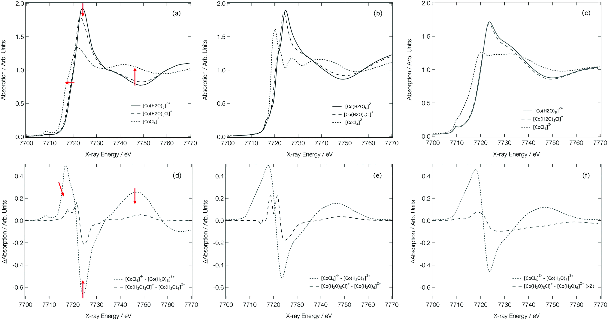 | ||
| Fig. 7 Experimental28 (a), FDMNES calculated (b) and DNN MD simulated (c) Co K-edge XANES spectra for [Co(H2O)6]2+, [Co(H2O)5Cl]+ and [CoCl4]2−. Experiment28 (d) FDMNES calculated (e) and DNN MD simulated (f) Co K-edge difference spectra for [CoCl4]2−–[Co(H2O)6]2+ and [Co(H2O)5Cl]+–[Co(H2O)6]2+. | ||
000 snapshots) at the DFT(ωB97X-D3)/def2-SVP level} and experiment {298 K; data reproduced from ref. 28}
| Co–O | Co–Cl | |||
|---|---|---|---|---|
| r avg. (Å) | σ 2 (Å2) | r avg. (Å) | σ 2 (Å2) | |
| [Co(H2O)6]2+ (333 K) | 2.063 | 0.009 | — | — |
| [Co(H2O)6]2+ (338 K) | 2.082 | 0.016 | — | — |
| [CoCl4]2− (333 K) | — | — | 2.312 | 0.007 |
| [CoCl4]2− (338 K) | — | — | 2.317 | 0.010 |
| [Co(H2O)5Cl]+ (333 K) | 2.068 | 0.006 | 2.386 | 0.007 |
| [Co(H2O)5Cl]+ (338 K) | 2.087 | 0.012 | 2.401 | 0.010 |
| [Co(H2O)6]2+ (298 K) | 2.077 ± 0.007 | 0.0087 ± 0.005 | — | — |
| [CoCl4]2− (298 K) | — | — | 2.272 ± 0.005 | 0.0060 ± 0.0003 |
| [Co(H2O)5Cl]+ (298 K) | 2.102 ± 0.009 | 0.0103 ± 0.0006 | 2.460 ± 0.037 | 0.0131 ± 0.0026 |
Fig. 7b shows the Co K-edge XANES spectra for [Co(H2O)6]2+, [Co(H2O)5Cl]+, and [CoCl4]2− as calculated using the FDM method at DFT(ωB97X-D3)/def2-SVP-optimised geometries. The optimised geometries of [Co(H2O)6]2+ and [Co(H2O)5Cl]+ have average Co–O bond lengths of 2.06 and 2.07 Å, respectively, and, for [Co(H2O)5Cl]+, and [CoCl4]2−, the average Co–Cl bond lengths are 2.30 and 2.32 Å, respectively; results which are in qualitatively-good agreement with the structural parameters tabulated in Table 1. The FDM-calculated XANES spectra for [Co(H2O)6]2+ and [Co(H2O)5Cl]+ are generally in good agreement with the experimental spectra shown in Fig. 7a. The FDM-calculated XANES spectrum of [CoCl4]2− can only be described as being in semi-quantitative agreement with experiment, but – crucially – all three of the main changes observed in the experimental XANES spectrum are reproduced in relative terms and, consequently, the FDM-calculated difference XANES spectra shown in Fig. 7e exhibit strong agreement with the experimental difference XANES spectra shown in Fig. 7d.
Fig. 7c shows the DNN-estimated XANES spectra obtained via sampling, estimating, and averaging snapshots from ab initio MD (at 333 K). Although the DNN-estimated spectra do not reproduce satisfactorily the strength of the white-line transition as observed in experiment, the trends noted in Fig. 7a are well reproduced, and this translates into DNN-estimated difference XANES spectra (shown in Fig. 7f) which nonetheless agree well with experiment. We stress that the differences occurring between Fig. 7b and c arise primarily due to the DNN and not, at this stage, through any effect of averaging snapshots from the ab initio MD. The most prominent difference is the weaker white-line transition, which is a consequence of the limitations of the muffin-tin-type potential approximation. Our DNN learns from absorption cross-sections that have been calculated under this approximation, this inherently limits the quality of the estimations that our DNN can produce at present. We have discussed this in detail, and recommended approaches that might be employed to remedy it, in ref. 46.
We now turn our attention to analysing the T-jump pump/X-ray probe data obtained 7 ns after arrival of the NIR T-jump pump pulse; these data are described in ref. 24 and reproduced in Fig. 8. It can be seen in Fig. 7d–f that both the experimental and calculated difference XANES spectra show a derivative profile consistent with a red shift of the absorption. This causes a mismatch between the experimental Co K-edge transient spectra shown in Fig. 8 that is acute below ca. 7725 eV. While caution has to be exercised, given the signal-to-noise ratio achieved in ref. 24, this point suggests that there is little-to-no change in the ratio of the Co complexes post-arrival of the T-jump NIR pump pulse and, therefore, that the dominant effect of the NIR pump pulse is not to change the position of the equilibrium in Fig. 1, but rather to simply heat the solution, i.e. drive an increase in the Debye–Waller factor and thermal disorder of the Co complexes already present at equilibrium {[Co(H2O)6]2+, [Co(H2O)5Cl]+, and [CoCl4]2−}.
 | ||
| Fig. 8 Experimental24 Co K-edge transient XANES spectrum (closed circles) obtained at 7 ns after application of a NIR pump laser compared with (a) simulated transient corresponding to [Co(H2O)6]2+ (338 K)–[Co(H2O)6]2+ (333 K), [Co(H2O)5Cl]+ (338 K)–[Co(H2O)5Cl]+ (333 K), and [CoCl4]2− (338 K)–[CoCl4]2− (333 K) combined in a ratio of 0.2:0.4:0.4, respectively. (b)–(d) show the individual components compared to experiment for [Co(H2O)6]2+, [Co(H2O)5Cl]+, and [CoCl4]2−, respectively. | ||
Fig. 8a shows the Co K-edge difference XANES spectrum upon 5 K heating for each of the complexes present at equilibrium – [Co(H2O)6]2+, [Co(H2O)5Cl]+, and [CoCl4]2− – combined in the ratio 0.2:0.4:0.4. The difference XANES spectra for each of these complexes individually are shown in Fig. 8b–d. The combined transient XANES spectrum, simulated via the ab initio MD strategy using 10000 snapshots for each Co complex at each temperature, shows good agreement with the experimental transient in terms of both lineshape and intensity; an impressive result, considering that the intensity change observed in the difference XANES spectrum corresponds to ca. 0.2% of the original spectral intensity. Indeed, capturing accurately the small difference between the XANES spectra is the reason why so many ab initio MD snapshots are necessitated; a high level of convergence is required. With reference to Table 1, the changes responsible for the observed difference spectrum are (i) a small elongation of the bonds in the Co complexes present at equilibrium, and (ii) a small associated increase in the Debye–Waller factors. We note that both are in good agreement with those reported in ref. 28. This agreement between experiment and theory for the transient spectrum shown in Fig. 8a, especially when compared to the transient spectra arising from both experimental and calculated data in Fig. 7, strongly supports that the structural changes following the T-jump are dominated by sample heating and a commensurate increase in the Debye–Waller factor rather than a change in the coordination environment.
4 Discussion and conclusions
In this Article, we have developed a DNN for the instantaneous prediction of XANES spectra at the Co K-edge, building on our recent work at the Fe K-edge.46,47 We have demonstrated that our DNN can predict Co K-edge XANES spectra using nothing more than the local geometry of the X-ray absorption site with consistent qualitative accuracy and that it can, in many cases, deliver quantitative (sub-eV) accuracy on peak positions with respect to reference XANES spectra. The structure and performance of the DNN optimised in the present Article is comparable to that reported in our recent work at the Fe K-edge,46,47 evidencing the potential transferability of our DNN to the K-edges of the other transition metal elements and, eventually, the extension of our model to encompass the rest of the periodic table.To trial our DNN for the first time in a practical setting, we have used it to analyse recent T-jump pump/X-ray probe experiments by Chergui et al. which focus on the NIR-driven ligand exchange processes of Co2+ in chlorinated aqueous solution.24 We have considered two possible outcomes post-arrival of the NIR T-jump pump pulse: (i) that the position of the equilibrium is forcibly shifted, either by the NIR-driven direct dissociation of a ligand or by an increase in the temperature that drives ligand exchange processes in which coordinated H2O molecules are exchanged for Cl− ions, or (ii) that the solution is simply heated, increasing the thermal disorder associated with the species present at equilibrium {[Co(H2O)6]2+, [Co(H2O)5Cl]+, and [CoCl4]2−} but otherwise leaving the position of the equilibrium between them unchanged.
One of the challenges here is to incorporate the effect of temperature into the simulations of the XANES spectra, and one of the strategies with which this can be achieved is to sample snapshots representatively from ab initio MD at a controlled temperature and calculate the Co K-edge XANES spectrum of each. Calculating the XANES spectra from first principles from many ab initio MD snapshots at an appropriate level of theory could take days. Our DNN facilitates exactly this kind of analysis by delivering fast (instantaneous) estimations of XANES spectra using nothing more than the local geometry of the X-ray absorption site; it is able to process thousands of ab initio MD snapshots in seconds. We stress that the purpose of our DNN is not to replace high-level calculations, but to complement them in situations such as this: our DNN can be used to take on cheaply and effectively the kind of analysis that is required here (i.e. an ab initio MD ensemble strategy) as a first step to eliminate improbable pathways quickly – high-level calculations can then be used to in a better-targeted way to deliver genuinely quantitative information.
Our DNN-assisted analysis suggests that, within the limit of the experimental signal-to-noise ratio, the transient XANES spectrum recorded in ref. 24 is dominated by the effects of a global temperature increase in the solution, leading to a small elongation of the bonds in the Co complexes present at equilibrium and a commensurate increase in the Debye–Waller factor, rather than any change in the ratio of the Co complexes post-arrival of the NIR T-jump pump pulse. This represents a promising first step towards the routine DNN-assisted analyses of XANES for disordered systems. However, further work is required to make this such DNN-assisted analyses practicable, despite the agreement between the predicted and experimental transients reported in the present Article. For example, the calculated XANES spectra in our reference dataset were obtained under the muffin-tin-type potential approximation – going beyond this approximate treatment represents a clear direction for future work, as the quality of the estimations that our DNN can make is inherently limited by the level of theory it has access to during the learning process. We acknowledge, however, that – even at the highest levels of theory – qualitative differences between experiment and theory can persist. Consequently, incorporating feedback on epistemic uncertainty in our DNN is also an aim for future work, so as to better quantify the range of practical applications that are reasonably within the scope of a DNN-assisted analysis.
With the advent of high-brilliance, 4th-generation light sources, e.g. X-ray free-electron lasers (XFELs), it is now possible to obtain insight into non-equilibrium/temperature-driven processes in disordered systems (e.g. amorphous systems, or in operando measurements of batteries and catalysts)66 over a large range of timescales, and these measurements are on course to become routine.67–69 Many geometric configurations have to be taken into account to correctly model the effects of disorder on measurements such as these,70 but performing high-level theoretical calculations for all of these geometric configurations is often precluded by time and resource requirements. We hope to see wider adoption of DNN-assisted analyses in the future since – as we have demonstrated in the present article – it provide an attractive and cost-effective route to the quantitative interpretation of these experiments.
Conflicts of interest
There are no conflicts to declare.Acknowledgements
The research described in this paper was funded by the Leverhulme Trust (Project RPG-2016-103) and EPSRC (EP/S022058/1, EP/R021503/1, and EP/R51309X/1). CDR is supported by a Doctoral Prize Fellowship (EP/R51309X/1). MMMM thanks Jazan university (KSA) for supporting her study and funding. This research made use of the Rocket High Performance Computing (HPC) service at Newcastle University. CDR additionally thanks the Alan Turing Institute, via which access to the EPSRC-supported (EP/T022205/1) Joint Academic Data Science Endeavour (JADE) HPC cluster was provided under Project JAD029.Notes and references
- A. H. Zewail, J. Phys. Chem. A, 2000, 104, 5660–5694 CrossRef CAS.
- R. Callender and R. B. Dyer, Curr. Opin. Struct. Biol., 2002, 12, 628–633 CrossRef CAS PubMed.
- S. Chen, I. S. Lee, W. A. Tolbert, X. Wen and D. D. Dlott, J. Phys. Chem., 1992, 96, 7178–7186 CrossRef CAS.
- C. D. Snow, L. Qiu, D. Du, F. Gai, S. J. Hagen and V. S. Pande, Proc. Natl. Acad. Sci. U. S. A., 2004, 101, 4077–4082 CrossRef CAS PubMed.
- P. Maiella and T. B. Brill, Appl. Spectrosc., 1996, 50, 829–835 CrossRef CAS.
- R. D. JiJi, G. Balakrishnan, Y. Hu and T. G. Spiro, Biochemistry, 2006, 45, 34–41 CrossRef CAS PubMed.
- G. Bunker, Introduction to XAFS: A Practical Guide to X-ray Absorption Fine Structure Spectroscopy, Cambridge University Press, 2010 Search PubMed.
- C. Rankine and T. Penfold, J. Phys. Chem. A, 2021 DOI:10.1021/acs.jpca.0c11267.
- N. Huse, H. Wen, D. Nordlund, E. Szilagyi, D. Daranciang, T. A. Miller, A. Nilsson, R. W. Schoenlein and A. M. Lindenberg, Phys. Chem. Chem. Phys., 2009, 11, 3951–3957 RSC.
- P. Wernet, G. Gavrila, K. Godehusen, C. Weniger, E. Nibbering, T. Elsaesser and W. Eberhardt, Appl. Phys., 2008, 92, 511–516 CAS.
- V.-T. Pham, T. J. Penfold, R. M. van der Veen, F. Lima, A. El Nahhas, S. L. Johnson, P. Beaud, R. Abela, C. Bressler and I. Tavernelli, et al. , J. Am. Chem. Soc., 2011, 133, 12740–12748 CrossRef CAS PubMed.
- T. J. Penfold, C. J. Milne, I. Tavernelli and M. Chergui, Pure Appl. Chem., 2012, 85, 53–60 Search PubMed.
- P. D’Angelo and V. Migliorati, J. Phys. Chem. B, 2015, 119, 4061–4067 CrossRef PubMed.
- M. Galib, G. Schenter, C. Mundy, N. Govind and J. Fulton, J. Chem. Phys., 2018, 149, 124503 CrossRef CAS PubMed.
- T. J. Penfold, M. Reinhard, M. H. Rittmann-Frank, I. Tavernelli, U. Rothlisberger, C. J. Milne, P. Glatzel and M. Chergui, J. Phys. Chem. A, 2014, 118, 9411–9418 CrossRef CAS PubMed.
- R. Ayala, E. S. Marcos, S. Daz-Moreno, V. A. Solé and A. Muñoz-Páez, J. Phys. Chem. B, 2001, 105, 7588–7593 CrossRef CAS.
- P. J. Merkling, A. Munoz-Páez, R. R. Pappalardo and E. S. Marcos, Phys. Rev. B: Condens. Matter Mater. Phys., 2001, 64, 092201 CrossRef.
- V. Pham, I. Tavernelli, C. Milne, R. van der Veen, P. DâĂŹAngelo, C. Bressler and M. Chergui, Chem. Phys., 2010, 371, 24–29 CrossRef CAS.
- J. L. Fulton, S. M. Heald, Y. S. Badyal and J. Simonson, J. Phys. Chem. A, 2003, 107, 4688–4696 CrossRef CAS.
- K. Henzler, E. O. Fetisov, M. Galib, M. D. Baer, B. A. Legg, C. Borca, J. M. Xto, S. Pin, J. L. Fulton and G. K. Schenter, et al. , Sci. Adv., 2018, 4, eaao6283 CrossRef PubMed.
- J. Chaboy and S. Daz-Moreno, J. Phys. Chem. A, 2011, 115, 2345–2349 CrossRef CAS PubMed.
- Y. Inada, H. Hayashi, K.-I. Sugimoto and S. Funahashi, J. Phys. Chem. A, 1999, 103, 1401–1406 CrossRef CAS.
- S. Daz-Moreno, A. Munoz-Paez, J. M. Martnez, R. R. Pappalardo and E. S. Marcos, J. Am. Chem. Soc., 1996, 118, 12654–12664 CrossRef.
- O. Cannelli, C. Bacellar, R. Ingle, R. Bohinc, D. Kinschel, B. Bauer, D. Ferreira, D. Grolimund, G. Mancini and M. Chergui, Struct. Dyn., 2019, 6, 064303 CrossRef CAS PubMed.
- H. Ma, C. Wan and A. H. Zewail, Proc. Natl. Acad. Sci. U. S. A., 2008, 105, 12754–12757 CrossRef PubMed.
- W. Liu, S. J. Borg, D. Testemale, B. Etschmann, J.-L. Hazemann and J. Brugger, Geochim. Cosmochim. Acta, 2011, 75, 1227–1248 CrossRef CAS.
- M. Uchikoshi, J. Solution Chem., 2018, 47, 2021–2038 CrossRef CAS.
- M. Uchikoshi and K. Shinoda, Struct. Chem., 2019, 30, 945–954 CrossRef CAS.
- P. Pan and N. J. Susak, Geochim. Cosmochim. Acta, 1989, 53, 327–341 CrossRef CAS.
- M. Reinhard, G. Auböck, N. A. Besley, I. P. Clark, G. M. Greetham, M. W. Hanson-Heine, R. Horvath, T. S. Murphy, T. J. Penfold and M. Towrie, et al. , J. Am. Chem. Soc., 2017, 139, 7335–7347 CrossRef CAS PubMed.
- J. Ojeda, C. A. Arrell, L. Longetti, M. Chergui and J. Helbing, Phys. Chem. Chem. Phys., 2017, 19, 17052–17062 RSC.
- O. Braem, T. J. Penfold, A. Cannizzo and M. Chergui, Phys. Chem. Chem. Phys., 2012, 14, 3513–3519 RSC.
- J. Timoshenko, D. Lu, Y. Lin and A. I. Frenkel, J. Phys. Chem. Lett., 2017, 8, 5091–5098 CrossRef PubMed.
- J. Timoshenko, A. Halder, B. Yang, S. Seifert, M. J. Pellin, S. Vajda and A. I. Frenkel, J. Phys. Chem. C, 2018, 122, 21686–21693 CrossRef CAS.
- J. Timoshenko, M. Ahmadi and B. R. Cuenya, J. Phys. Chem. C, 2019, 123, 20594–20604 CrossRef CAS.
- M. Ahmadi, J. Timoshenko, F. Behafarid and B. R. Cuenya, J. Phys. Chem. C, 2019, 123, 10666–10676 CrossRef CAS PubMed.
- J. Timoshenko, C. J. Wrasman, M. Luneau, T. Shirman, M. Cargnello, S. R. Bare, J. Aizenberg, C. M. Friend and A. I. Frenkel, Nano Lett., 2019, 19, 520–529 CrossRef CAS PubMed.
- J. Timoshenko and A. I. Frenkel, ACS Catal., 2019, 9, 10192–10211 CrossRef CAS.
- Y. Liu, N. Marcella, J. Timoshenko, A. Halder, B. Yang, L. Kolipaka, M. J. Pellin, S. Seifert, S. Vajda, P. Liu and A. I. Frenkel, J. Chem. Phys., 2019, 151, 164201 CrossRef PubMed.
- O. Trejo, A. L. Dadlani, F. De La Paz, S. Acharya, R. Kravec, D. Nordlund, R. Sarangi, F. B. Prinz, J. Torgersen and N. P. Dasgupta, Chem. Mater., 2019, 31, 8937–8947 CrossRef CAS.
- M. R. Carbone, S. Yoo, M. Topsakal and D. Lu, Phys. Rev. Mater., 2019, 3, 033604 CrossRef CAS.
- M. R. Carbone, M. Topsakal, D. Lu and S. Yoo, Phys. Rev. Lett., 2020, 124, 156401 CrossRef CAS PubMed.
- O. A. Usoltsev, A. L. Bugaev, A. A. Guda, S. A. Guda and A. V. Soldatov, Top. Catal., 2020, 63, 58–65 CrossRef CAS.
- A. A. Guda, S. A. Guda, A. Martini, A. L. Bugaev, M. A. Soldatov, A. V. Soldatov and C. Lamberti, Radiat. Phys. Chem., 2020, 175, 108430 CrossRef CAS.
- C. Zheng, C. Chen, Y. Chen and S. P. Ong, Patterns, 2020, 1, 100013 CrossRef PubMed.
- C. D. Rankine, M. M. Madkhali and T. J. Penfold, J. Phys. Chem. A, 2020, 124, 4263–4270 CrossRef CAS PubMed.
- M. M. Madkhali, C. D. Rankine and T. J. Penfold, Molecules, 2020, 25, 2715 CrossRef CAS PubMed.
- XANESNET, 2021, gitlab.com/conor.rankine/xanesnet, commit: 61deec3f.
- J. Gasteiger, J. Schuur, P. Selzer, L. Steinhauer and V. Steinhauer, Fresenius’ J. Anal. Chem., 1997, 359, 50–55 CrossRef CAS.
- M. C. Hemmer, V. Steinhauer and J. Gasteiger, J. Vib. Spectrosc., 1999, 19, 151–164 CrossRef CAS.
- M. C. Hemmer and J. Gasteiger, Anal. Chim. Acta, 2000, 420, 145–154 CrossRef CAS.
- O. A. von Lilienfeld, R. Ramakrishnan, M. Rupp and A. Knoll, Int. J. Quantum Chem., 2015, 115, 1084–1093 CrossRef CAS.
- K. Hansen, G. Montavon, F. Biegler, S. Fazli, M. Rupp, M. Scheffler, O. A. Von Lilienfeld, A. Tkatchenko and K.-R. Müller, J. Chem. Theory Comput., 2013, 9, 3404–3419 CrossRef CAS PubMed.
- M. Abadi, A. Agarwal, P. Barham, E. Brevdo, Z. Chen, C. Citro, G. S. Corrado, A. Davis, J. Dean, M. Devin, S. Ghemawat, I. Goodfellow, A. Harp, G. Irving, M. Isard, Y. Jia, R. Jozefowicz, L. Kaiser, M. Kudlur, J. Levenberg, D. Mane, R. Monga, S. Moore, D. Murray, C. Olah, M. Schuster, J. Shlens, B. Steiner, I. Sutskever, K. Talwar, P. Tucker, V. Vanhoucke, V. Vasudevan, V. Fernanda, O. Vinyals, P. Warden, M. Wattenberg, M. Wicke, Y. Yu and X. Zheng, TensorFlow: Large-Scale Machine Learning on Heterogeneous Distributed Systems, 2015, tensorflow.org.
- Keras, 2015, http://github.com/keras-team/keras.
- GPy: A Gaussian Process Framework in Python, 2012, github.com/SheffieldML/GPy.
- GPyOpt: A Bayesian Optimization Framework in Python, 2016, github.com/SheffieldML/GPyOpt.
- A. Jain, S. P. Ong, G. Hautier, W. Chen, W. D. Richards, S. Dacek, S. Cholia, D. Gunter, D. Skinner, G. Ceder and K. A. Persson, APL Mater., 2013, 1, 011002 CrossRef.
- S. P. Ong, S. Cholia, A. Jain, M. Brafman, D. Gunter, G. Ceder and K. A. Persson, Comput. Mater. Sci., 2015, 97, 209–215 CrossRef.
- O. Bunău and Y. Joly, J. Phys.: Condens. Matter, 2009, 21, 345501 CrossRef PubMed.
- M. Seah and W. Dench, NPL Rep. Chem, 1978, 82, 10 Search PubMed.
- Y. Shao, Z. Gan, E. Epifanovsky, A. T. Gilbert, M. Wormit, J. Kussmann, A. W. Lange, A. Behn, J. Deng and X. Feng, et al. , Mol. Phys., 2015, 113, 184–215 CrossRef CAS.
- J.-D. Chai and M. Head-Gordon, Phys. Chem. Chem. Phys., 2008, 10, 6615–6620 RSC.
- F. Weigend and R. Ahlrichs, Phys. Chem. Chem. Phys., 2005, 7, 3297–3305 RSC.
- K. Waizumi, T. Kouda, A. Tanio, N. Fukushima and H. Ohtaki, J. Solution Chem., 1999, 28, 83–100 CrossRef CAS.
- J. Timoshenko and B. Roldan Cuenya, Chem. Rev., 2021, 121, 882–961 CrossRef CAS PubMed.
- T. Penfold, C. Milne and M. Chergui, Adv. Chem. Phys., 2013, 153, 1–41 CAS.
- P. M. Kraus, M. Zürch, S. K. Cushing, D. M. Neumark and S. R. Leone, Nat. Rev. Chem., 2018, 2, 82–94 CrossRef CAS.
- M. Khalil and S. Mukamel, J. Chem. Phys., 2020, 153, 100401 CrossRef CAS PubMed.
- G. Capano, C. Milne, M. Chergui, U. Rothlisberger, I. Tavernelli and T. Penfold, J. Phys. B: At., Mol. Opt. Phys., 2015, 48, 214001 CrossRef.
Footnote |
| † The data supporting this publication are openly available under an Open Data Commons Open Database License. Additional metadata are available at DOI: http://10.25405/data.ncl.12966776. |
| This journal is © the Owner Societies 2021 |