A comprehensive optimization study on Bi2Te3-based thermoelectric generators using the Taguchi method†
Received
8th September 2017
, Accepted 4th October 2017
First published on 1st November 2017
Abstract
Low-grade waste heat recovery is a promising source of renewable energy; however, there are practical challenges in the recovery process. Thermoelectric generators (TEGs) are a viable solution, but their efficiency remains low, thereby limiting their implementation. The performance of TEGs can be enhanced by optimizing the module configuration; however, optimizing all the parameters experimentally using traditional experimental techniques will require several trials, and therefore, it is cumbersome and expensive. Here, we demonstrate the Taguchi method for optimizing TEG modules and demonstrate that full optimization can be achieved in just 25 experiments. The optimization has been achieved in four stages. In the first stage, a numerical model of thermoelectricity is developed and used in the second stage to optimize key geometric parameters of TEGs through the Taguchi method. In the third stage, the Taguchi method is used to optimize the geometric dimensions of the heat sink. Lastly, in the fourth stage, the effect of operating conditions on the performance of TEGs is investigated. The results reveal that the Taguchi method is capable of predicting the near-optimal configuration of TEGs.
Introduction
More than half of the total energy generated from various sources is rejected as waste heat.1 Waste heat should be recovered in order to enhance the process efficiencies; however, there are practical challenges because of the fact that heat rejection occurs in varying forms, such as high-grade, medium-grade, or low-grade and varying modes, such as conduction, convection, and radiation.1,2 The lower the average temperature, the more complex and expensive is the waste heat recovery. The U.S. Department of Energy estimates that the low-grade waste heat (hot-side temperature less than 230 °C) constitutes 60% of the total rejected energy from the industrial sector.3 Forman et al.1 estimated that 79% of the world's total waste heat occurs at a temperature below 299 °C. Some of the current technologies used to convert thermal energy into other more usable forms (such as electrical or mechanical energy) are based on thermoelectric, pyroelectric, thermomagnetic, thermo-acoustics, and shape-memory alloy based generators. Out of all these choices, thermoelectric generators (TEGs) are considered as the most mature technology. TEGs are solid-state devices with no moving parts or any harmful chemical discharge and they convert heat directly into electricity. However, the low efficiency of TEGs, especially at operating temperatures less than 200 °C, is a concern. In the past few decades, there have been numerous attempts towards the development of high performance thermoelectric (TE) materials, but the performance of TEGs remains below the desired range.4,5
The performance of TE materials is measured in terms of the non-dimensional figure-of-merit, ZT, defined as5
where
α is the Seebeck coefficient,
σ is the electrical conductivity,
κ is the thermal conductivity, and
T is the absolute temperature.
Theoretically, an efficient TE material should have a high Seebeck coefficient, high electrical conductivity, and low thermal conductivity. However, for most materials, thermal and electrical conductivities are directly related and these properties increase or decrease in the same manner. Also, the Seebeck coefficient and electrical conductivity vary reciprocally, causing difficulties in achieving any drastic improvement in the figure of merit ZT.5,6 Improvement in material performance has to be complemented with improvement in module design to achieve higher device level ZT. The thermal-to-electrical energy conversion efficiency of a TEG is defined as
| |  | (2) |
where
Pout is the electrical power produced and
Qin is the heat flow rate from a heat source to the hot-side of a TEG.
For a TEG operating between fixed hot-side and cold-side temperatures, Th and Tc, there exists an optimal external load, where the output power is maximum. The maximum energy conversion efficiency of an ideal TEG operating under the optimal conditions is given in terms of ZT as:7
| | 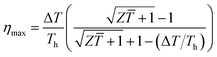 | (3) |
where Δ
T is the temperature difference across the TE module and
![[T with combining macron]](https://www.rsc.org/images/entities/i_char_0054_0304.gif)
is the mean operating temperature in kelvin.
Some of the conventional TE materials include bismuth telluride (Bi2Te3), lead telluride (PbTe), silicon germanium (SiGe), and cobalt triantimonide (CoSb3) based skutterudites. The selection of a suitable material depends upon the hot-side temperature of the source. Most of the conventional TE materials possess average ZT less than unity in low temperature regime. In applications below 200 °C, such as that for low-grade waste heat recovery, Bi2Te3-based alloys are the optimum TE materials. Bi2Te3 alloyed with Sb and Se has slightly higher average ZT than the unmodified material, but the average value is still close to unity in the low temperature regime. Some techniques such as nanostructuring,8–13 doping with Cu or Ag atoms,14,15 and adjusting the atomic ratio of Sb/Bi atoms16 have been found to improve the ZT of Bi2Te3-based TE materials. Hao et al.17 have demonstrated that by suppressing the intrinsic excitation in Bi2Te3-based TE materials through addition of a small amount of electron acceptors such as Cd, Cu, and Ag lowers the lattice thermal conductivity and increases the ZT. The study further demonstrated that compound Bi0.5Sb1.5−xCuxTe3 (x = 0.005) has a maximum ZT of 1.4 and an average ZT of 1.2 between 100 and 300 °C. The TEG module fabricated using this material was found to exhibit an energy conversion efficiency up to 6.0% with a hot-side temperature of 512 K and a cold-side temperature of 295 K, which was about 30% higher than the non-optimized BiTe-based modules.
TEGs broadly consist of three main components: p-type and n-type TE legs, conductive electrodes that connect the TE legs electrically in series and thermally in parallel, and ceramic plates on two sides to electrically insulate the TE module. In addition, TEGs may also have metallic fins as the heat sink on the cold-side to dissipate the heat to the surroundings or to the cooling fluid. The performance of TEGs, not only depends on the ZT of the TE material but also on the operating conditions and configuration of the TE module. The operating conditions include the heat source and heat sink temperatures, the modes of heat transfer, and the environmental conditions such as ambient temperature, pressure, wind speed, and humidity. In addition, TEGs also have an optimal electric load where the device has the best performance. The performance of TEGs can be enhanced through three possible ways. First, by improving ZT of the thermoelectric materials. Second, by optimizing the geometric parameters of TEG modules, such as the number of p–n legs, leg length and cross-sectional area, and third, by optimizing the modes of heat transfer, which includes design improvement in the heat exchanger and heat sink. TE devices have been extensively examined analytically, numerically, and experimentally in the past to optimize both geometric parameters and operating conditions. Niu et al.,18 Hsu et al.,19 and Gou et al.20 have presented experimental studies on low-temperature TEGs for waste heat recovery. These studies have provided promising results indicating the potential for harvesting energy from low-temperature waste heat sources, especially from industrial waste. However, evaluating the influence of all the operating conditions and geometric parameters requires numerous experimentation; therefore, experimental studies on TE devices are often substantiated by analytical and numerical modelling, which can either be a simplified one-dimensional model21,22 or a complex three-dimensional model.23–26 A significant amount of research related to the optimization of p–n leg geometry, i.e. the length,27 the cross-sectional area,28 and the number of thermocouples,29 can be found in the literature. Some of the prior studies have focused on finding the length to the cross-sectional area ratio to determine the optimum shape parameter,30 aspect ratio (leg length/leg area),31 and slenderness ratio ((Ap/Lp)/(An/Ln))32 of the p–n thermocouple. While high efficiency was found to occur when the length of the couple was large, output power was obtained at some intermediate value.33 For micro-thermoelectric generators, output power was found to decline with the cross-sectional area of the thermocouples, whereas efficiency was found to exhibit an opposite trend.34 In addition, since n-type telluride-based materials are usually weaker than their p-type counterparts, a slenderness ratio less than one was suggested for the peak performance of the TEG modules.35 There have been attempts36–38 on coupling the thermoelectric equations with the heat transfer equations of the heat sink in order to simultaneously optimize the TEG and heat sink geometries. The results have shown that the performance of TEGs is highly dependent on leg dimensions along with heat sink geometry and the method of heat transfer from the heat source/sink to the TE modules. In order to reduce the complexity in the TE module design and minimize the design parameters, various modelling techniques have been proposed. Fraisse39 attempted to study the leg geometry using thermoelectric element modelling based on an electrical analogy. Cheng and Lin40 proposed genetic algorithms (GAs) for geometric optimization of thermoelectric coolers in a confined volume. Another design method based on dimensional analysis for optimizing thermoelectric devices was developed by Lee41 and Yamanashi.42 Huang43 proposed a simplified conjugate-gradient method for geometry optimization of thermoelectric coolers. These previous studies have provided several insights into modelling of the TEGs and proposed pathways for understanding the role of controlling parameters. In practice, designers need a modelling methodology that can provide a near-optimum TEG configuration in the least number of trials. This not only saves time and resources but also improves the robustness as a diverse set of materials can be investigated in a rapid manner under varying operating conditions. Here we address this need through implementation of the Taguchi method. We believe that this methodology will provide a toolset for the design of modules to a broader community attempting to utilize thermoelectric materials.
In this study, we utilize thermal and electrical properties of a high performance Bi0.5Sb1.5−xCuxTe3 (x = 0.005) alloy reported by Hao et al.17 and numerically simulate the performance of TEGs built using this composition under different geometric and operating conditions. The Taguchi method of optimization is a statistical tool that predicts the optimal performance with far less number of trials than the conventional optimization techniques, where only one factor is normally varied at a given instance. The Taguchi optimization method allows us to vary multiple factors at a given instance in a controlled manner, thereby reducing the total number of trials required. This method is widely used in diverse fields of research and engineering, such as manufacturing processes,44–47 thermal analysis,48–50 and chemical and biochemical studies.51–53 Chen et al.54 used the Taguchi method to optimize the dimensions, length, width, and height, of the heat sink along with the hot-side temperature and resistive load for TEGs. An n-type polycrystalline silicon layer for a micro thermoelectric generator (TEG) was designed using the Taguchi method by Kim et al.55 Kishore et al.56 have applied the Taguchi method to optimize the cooling capacity and coefficient of performance of thermoelectric coolers.
Here, we demonstrate the optimization of TEGs in four subsequent stages. In the first stage, we validate the numerical model using published experimental data and then investigate the effect of contact resistances on the output power and efficiency. In the second stage, the geometric parameters of TEGs, namely the cross-sectional area and height of p–n legs, along with the resistive load are optimized using Taguchi method. In the third stage, the Taguchi method is used to optimize the geometric parameters of the heat sink. In the fourth and last stage, we study the effect of operating conditions, more specifically the total heat transfer coefficient and the ambient temperature, on the performance of TEGs.
Governing equations and numerical modelling
Modelling a TEG requires coupling four different thermal–electrical phenomena: Joule heating, the Seebeck effect, the Peltier effect, and the Thomson effect. There are several analytical and numerical models proposed in the literature to study TEGs,23,57–61 but broadly, these models are based on the principle of conservation of energy and continuity of electric charge. Based upon a one-dimensional theoretical model, the output voltage, Vm, and current, Im, of a TEG module, when it is operated with a matched load, are given as:21| | 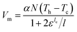 | (4) |
| | 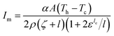 | (5) |
where N is the number of p–n legs, A is the leg cross-sectional area, l is the leg length, lc is the thickness of the contact layer, ρ is the electrical resistivity, λ is the thermal resistivity, ρc is the electrical contact resistivity, λc is the thermal contact resistivity, ζ = λ/λc and ε = 2ρ/ρc.
The output power P and efficiency η are given as:21
| | 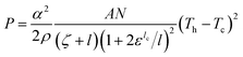 | (6) |
| |  | (7) |
The one-dimensional analytical equations presented above are valid under a small temperature gradient and constant thermoelectric properties. In order to account for temperature-dependent TE properties at a larger temperature difference, the coupled thermoelectric equations need to be solved. The coupled thermal–electrical governing equations in the steady-state are given as62
| |  | (8) |
| |  | (9) |
where vectors
represent the heat flux, electric current density, electric field, and thermal gradient, respectively. The Seebeck coefficient
α and Peltier coefficient π are related as π =
Tα. We have used commercial finite element analysis (FEA) code ANSYS v17.0 (ANSYS Inc., USA) to numerically solve the thermoelectric constitutive equations. ANSYS deduces the thermoelectric constitutive
eqn (8) and
(9) in the form of a finite element matrix equation of thermoelectricity given as
63| |  | (10) |
where [
Ct] and [
Cv] are the finite element specific heat matrix and dielectric permittivity coefficient matrix, respectively; [
Kt], [
Kv], and [
Kvt] are the finite element thermal conductivity matrix, electrical conductivity coefficient matrix, and Seebeck coefficient coupling matrix, respectively; {
Q} denotes the sum of finite element heat generation load and convection surface heat flow vectors; {
Qp} is the finite element Peltier heat load vector; {
T}, {
V}, and {
I} are the vectors of the finite element nodal temperature, nodal electric potential, and nodal current, respectively. More details can be found elsewhere.
63
The discretization technique and mesh independency test
Fig. 1(a) shows the three-dimensional CAD model of the TEG module generated using ANSYS DesignModeler. The overall dimension, 30 × 30 × 3.5 mm3, of the TEG model is the same as that of TEG modules used in ref. 17. Seventy-one pairs of p–n legs of size 1.5 × 1.5 × 1.7 mm3 were assembled electrically in series and thermally in parallel using copper electrodes of thickness 0.1 mm. Ceramic substrates were added on both sides to electrically isolate the TE module. SOLID226 (a 3D 20-node hexahedron/brick) elements were used to discretize the FEA model. Constant temperature thermal boundary conditions were considered on the hot-side and cold-side of the TEG module. Heat loss along the side surfaces of p–n legs is ignored in the initial stage. As shown in Fig. 2, ground voltage is prescribed as the electrical boundary condition on the two free ends of copper electrodes including the external resistor. Due to nonlinearity of the governing equations, the full Newton–Raphson scheme has been used to obtain the finite element solution.
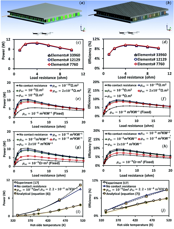 |
| | Fig. 1 (a) CAD model of a TEG with overall dimensions of 30 × 30 × 3.5 mm3, containing 71 pairs of p–n legs of size 1.5 × 1.5 × 1.7 mm3. (b) Medium-size mesh structure used for the simulation, element type: SOLID226 (3D 20-node hexahedron/brick). (c) Mesh independency test, comparing output power at three different element counts. (d) Mesh independency test, comparing efficiency at three different element counts. (e) Effect of electrical contact resistance on output power. (f) Effect of electrical contact resistance on efficiency. (g) Effect of thermal contact resistance on output power. (h) Effect of thermal contact resistance on efficiency. (i) Comparison among analytical, numerical, and experimental results for output power. (j) Comparison among analytical, numerical, and experimental results for efficiency. | |
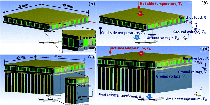 |
| | Fig. 2 (a) Key geometric parameters of the TEG module. The overall area of the TEG module is fixed to be 30 mm × 30 mm. The length, L, and width, W, of p–n legs are considered equal and varied together; whereas, the height, H, of the p–n legs is varied independently to optimize the leg geometry. (b) Boundary conditions of the TEG model used in the first step of optimization. (c) Key geometric parameters of the heat sink. The gap, b, between the fins is fixed to be 0.5 mm, whereas fin thickness, a, and the height, c, are varied along with the external resistive load. (d) Boundary conditions of the numerical model used for the second step of optimization. | |
As part of the mesh independency test, we varied the element count by refining the mesh size at three stages. The mesh independency test is essential to ensure that the numerical results are independent of the grid size. Fig. 1(b) depicts the medium-size mesh structure with an element count of 12129. The temperature dependent material properties of the TE material Bi0.5Sb1.5−xCuxTe3 (x = 0.005) from the literature17 have been used for all the calculations. For the mesh independency test, the hot-side and cold-side temperatures were fixed at 513 K and 295 K, respectively. Fig. 1(c) and (d) depict the numerical results for output power and efficiency versus load resistance obtained at three different element counts. The maximum change in results between the first case (element count # 7760) and the second case (element count # 12129) was found to be around 1.7% for output power and 2.0% for efficiency. The maximum change in results between the second case (element count # 12129) and the third case (element count # 33960) was found to be less than 0.1%. Therefore, we have used a medium-size meshing strategy in the rest of paper.
Effect of contact resistance
Contact resistance occurs at the contacting interface of two similar or dissimilar materials. It leads to an increase in the total resistance of the system and decreases the performance. In the case of TEGs, the contact resistance occurs at the interface between the p–n legs and the copper electrodes and at the interface between the copper electrodes and the ceramic substrates. The electrical contact resistance, ρec, typically lies in the range of 1.0 × 10⁻⁹ to 1.0 × 10⁻⁷ Ω m2, whereas, the thermal contact resistance, ρtc, has been reported to have typical values in the range of 1.0 × 10⁻⁶ to 1.0 × 10⁻⁴ m2 K W−1.64–67Fig. 1(e) and (h) show the effect of electrical and thermal contact resistances on the output power and efficiency of TEGs. Fig. 1(e) and (f) show the variation in output power and efficiency at different values of electrical contact resistance between 0 and 1.0 × 10⁻⁸ Ω m2 (thermal contact resistance is fixed at 1.0 × 10⁻⁶ m2 K W−1). It can be noted that TEG performance is highest when there is no electrical contact resistance. Output power and efficiency decrease gradually with an increase in electrical contact resistance. Increasing the electrical contact resistance from 0 to 1.0 × 10⁻⁸ Ω m2 reduces the peak output power by 47% and peak efficiency by 37%. Fig. 1(g) and (h) show the variation in output power and efficiency at different values of thermal contact resistance between 0 and 2.0 × 10⁻⁴ m2 K W−1 (electrical contact resistance is fixed at 1.0 × 10⁻⁹ Ω m2). TEG performance is highest when there is no thermal contact resistance. Similar to electrical contact resistance, thermal contact resistance also has an adverse effect on the output power and efficiency of TEGs. Increasing the thermal contact resistance from 0 to 2.0 × 10⁻⁴ m2 K W−1 reduces the peak output power by 61% and peak efficiency by 35%.
Validation of the numerical model
In order to validate the finite element model, the numerical results were compared with the analytical results obtained using a one-dimensional model (eqn (6) and (7)) and the experimental results obtained from the literature.17Fig. 1(i) and (j) show this comparison. The cold-side temperature is fixed at 295 K, whereas, the hot-side temperature is varied between 333 K and 513 K. It is important to note that the thermoelectric properties of TE materials vary with temperature, but it is cumbersome to account this in the analytical model. Therefore, we have used an average value of the Seebeck coefficient, thermal conductivity, and electrical conductivity for analytical calculation. Contact resistances have been ignored in this calculation; however, in the numerical model, temperature dependent thermoelectric properties as well as contact resistances have been used. As shown in Fig. 1(i) and (j), assuming no contact resistances, the numerical results and analytical results are close with a maximum deviation of 12% in output power at 513 K. A large deviation at high temperature is expected because the one-dimensional analytical model is effective at a small thermal gradient and with constant material properties. It can be observed that for the given electrical contact resistance ρec = 1.0 × 10⁻⁹ Ω m2 and thermal contact conductance ρtc = 2.2 × 10⁻⁴ m2 K W−1, the numerical and experimental results are in close agreement. The difference in the values for output power and efficiency at Th = 513 K was found to be 1.6% and 2.1%, respectively. Therefore, for all the simulations conducted in remainder of the paper, a constant electrical contact resistance of 1.0 × 10⁻⁹ Ω m2 and thermal contact resistance of 2.2 × 10⁻⁴ m2 K W−1 have been considered.
Taguchi method of optimization
Traditional optimization techniques are based on a full factorial design approach, where only one process factor is normally changed at a time and the output response is recorded. Varying each process factor at all possible levels makes the optimization process cumbersome and costly. The process cost and complexity further increase with an increase in either the number of factors or their levels or both. To overcome this problem, Taguchi68 introduced a statistical technique, called Taguchi's robust design method, more commonly known as the Taguchi optimization method, which suggests a partial factorial design of optimization based on some standard orthogonal arrays. The orthogonal arrays allow us to vary the process factors in few given combinations, thereby reducing the total number of trials required. Though the Taguchi method was originally developed for manufacturing industries to optimize the product quality and to minimize the production cost, more recently, this method has been often used in diverse fields of engineering.44–46,48–53 The detailed procedure to apply the Taguchi optimization method can be found in the literature,69 but broadly this method involves steps described in the sections below.
Objective function
The objective of the Taguchi optimization process is to determine an optimized setting of the process factors that provides an optimal output result. The objective of the present work is to maximize the output power and efficiency of TEGs.
Process factors and their levels
The process factors that affect the performance of a system can be divided into two categories: (i) control factors and (ii) noise factors. Control factors are process factors that can be controlled and adjusted by the operator, whereas, the noise factors occur due to environmental effects or due to other uncontrollable events that are difficult to be regulated. The Taguchi optimization method identifies the control factors that minimize the effect of noise factors on the system's output and improves the consistency in performance. Some of the control factors that affect the output power and efficiency of a TEG are the geometric parameters of the p–n legs, geometric parameters of the heat sink, operating temperature, total heat transfer coefficient, and external resistive load. Some of the noise factors, on the other hand, can be ambient temperature, atmospheric pressure, humidity and wind speed.
Selection of an appropriate orthogonal array
Orthogonal arrays identify the combination in which the control factors are varied during optimization trials. Some of the standard orthogonal arrays used in the Taguchi optimization method are L4, L8, L9, L12, L16, L18, and L25. Selection of an appropriate orthogonal array depends on the number of control factors and their levels. In this study, we have used an L25 orthogonal array whose structure is shown in Table S1 in the ESI document.† Ideally, an L25 orthogonal array should have 5 factors with 5 levels each, but a lower number of factors can also be used. Here, we have used only 3 factors at a time. It is important to note that with 5 factors at 5 levels, the traditional optimization method requires 55 = 3125 trials; whereas, the Taguchi method, per L25 orthogonal array, needs only 25 trials to predict the optimal output.
Optimization trials
Once the most appropriate orthogonal array is decided, the optimization process starts and the control factors are changed in the combinations shown in the orthogonal array. In this study, computational trials were performed as per the standard L25 array shown in Table S1.†
Signal-to-noise ratio
In the Taguchi optimization method, the desirable component of the output response is measured in terms of signal; whereas, the undesirable component is measured in terms of noise, which occurs due to variability in the process due to noise factors.46,69 Higher the value of the signal-to-noise (S/N) ratio, higher is the effect of control factors over the noise factors on the output. Depending upon the optimization goal, there are usually three ways to calculate the S/N ratio: larger is better, smaller is better, and nominal is best. Detailed formulation of three types of signal-to-noise ratios is provided in the ESI document.† In this study, the goal is to maximize output power and efficiency; therefore, the larger is better concept for the S/N ratio is used, which is calculated using the equation:| |  | (11) |
where r is the number of data points and yi is the value of the ith data point. A higher value of the larger is better S/N ratio identifies a setting of the control factors that minimizes the effects of the noise factors, thereby making the process robust to variation caused by the noise factors. In the Taguchi method, optimization is achieved using a 2-step process. In the first step, the larger is better S/N ratio is used to identify the level of control factors that reduces variability. In the second step, we identify those control factors that move the mean close to the target and have a minimal effect on the S/N ratio.70
Analysis of variance (ANOVA)
ANOVA stands for analysis of variance. It is a statistical technique used to compare the variation in result caused by the control factors and the error term relative to the total variation observed. The error term signifies the collective effect of all the external factors not considered in the study, including experimental error and noise factors. A typical ANOVA table contains the degrees of freedom (DOF), the sum of squares (SS), variance (V), and percentage contribution (P) for each control factor and for the error term. Detailed formulation for ANOVA is given in the ESI document.† In this study, we have used the commercial program Minitab 17 (Minitab Inc., USA) to obtain the ANOVA table.
Predicting the optimal output and the confirmation run
After the optimal control factors are obtained using the S/N ratios, the optimal output Y is predicted using the equation:71| |  | (12) |
where ![[X with combining macron]](https://www.rsc.org/images/entities/i_char_0058_0304.gif) i denotes the mean of the output results at the optimal level of factor i, denotes the grand mean of all the output data, and m represents the total number of control factors. The confidence interval (CI) at a certain confidence level (1 − α) for the predicted output is calculated using46
i denotes the mean of the output results at the optimal level of factor i, denotes the grand mean of all the output data, and m represents the total number of control factors. The confidence interval (CI) at a certain confidence level (1 − α) for the predicted output is calculated using46| | 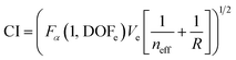 | (13) |
where Fα(1, DOFe) denotes the F-ratio at the confidence level of (1 − α) against a DOF of 1 and the error degree of freedom, DOFe. This value can be obtained from the F-table provided in a standard statistical book. Ve denotes the error variance, which is obtained from the ANOVA table. R denotes the number of repeated runs for the confirmation, and neff is the effective number of replications, which is calculated using46| | 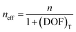 | (14) |
where n denotes the total number of experiments and (DOF)T is the total degree of freedom in the estimation of mean. The confirmation run is performed at the optimal levels of control factors and the obtained output result is compared against the predicted output. The actual output should fall in the range: (Ypredicted − CI) ≤ Yactual ≤ (Ypredicted + CI).
Optimization strategy
The optimization of the TEG was achieved in three consecutive steps. In the first step, we optimized the geometric dimensions of p–n legs using the Taguchi method, followed by validation of the results obtained using the full-factorial design of optimization. In the second step, the geometric dimensions of the heat sink (fin dimensions) were optimized using the Taguchi method. These results were then validated against the data obtained from the full-factorial design. Finally, we performed the performance characterization of the optimized TEG module under different operating conditions (cooling coefficient and ambient temperature).
Fig. 2(a) and (b) show the key geometric parameters and the boundary conditions for the TEG module considered in the first step of the optimization study. The overall area of the TEG module was fixed to be 30 mm × 30 mm. The height of the module varies with the change in the height of p–n legs. The thickness of the copper electrode was fixed at 0.1 mm and the ceramic substrates had 0.8 mm thickness. The gap distance among p–n legs is fixed at 0.15 mm. A constant electrical contact resistance of 1.0 × 10⁻⁹ Ω m2 and thermal contact resistance of 2.2 × 10⁻⁴ m2 K W−1 are considered. The length, L, and width, W, of p–n legs are considered equal and varied together; whereas, the height, H, of the p–n legs is varied independently to optimize the leg geometry. The number of p–n legs also changes with change in cross-sectional area and can be calculated using the model. In addition to the geometric parameters, the resistive load also has a strong effect on the performance of TEGs; therefore, it needs to be varied. The hot-side temperature, Th and the cold-side temperature, Tc are fixed at 513 K and 295 K, respectively, in this case.
Fig. 2(c) and (d) show the key geometric parameters and the boundary conditions of the heat sink considered in the second step of the optimization study. The geometric dimensions of p–n legs are fixed based on the results obtained from the first step. Other parameters such as the thickness of the copper electrode and ceramics substrates and contact resistances are the same as mentioned in the first step. The heat sink is assumed to be made up of aluminum and the thermal contact resistance between the ceramic substrate and the aluminum base is assumed to be 2.2 × 10⁻⁴ m2 K W−1.72 The gap, b, between the fins is fixed to be 0.5 mm, whereas fin thickness, a, and the height, c, are varied along with the external resistive load. The number of fins also changes with change in its cross-sectional area, which can be calculated since the overall size of the TEG module is fixed. The hot-side temperature is fixed at 513 K and a constant total heat transfer coefficient of 20 W m−2 K−1 is considered on the cold-side. The ambient temperature is fixed at 295 K. Table S2 in the ESI document† shows the different steps followed during the optimization process, the overall objective, and the range of parameters considered.
Results and discussion
Optimizing the geometric parameters of TEGs
Table 1 shows the control factors and their levels considered for Taguchi optimization. The control factors include two geometric parameters (cross-sectional area and height) of p–n legs and the resistive load. Selection of control factors was finalized after conducting a detailed literature review on the optimization of TEGs. In order to determine the range or the levels in which each control factor needs to be varied, some initial screening simulations were conducted to identify the direction in which the optimization occurs. Table 2 shows the number of simulation trials and the combination in which control factors are varied per L25 orthogonal array. The TEG output response: the output power (P) and efficiency (η) obtained from each trial are given in the 5th and 7th columns, respectively. “Larger is better” signal-to-noise ratios, S/NP for power and S/Nη for efficiency were also calculated using eqn (7) and are shown in the 6th and 8th columns, respectively.
Table 1 Control factors and their levels considered for geometric optimization of TEGs
| Control factors |
Levels |
| (1) |
(2) |
(3) |
(4) |
(5) |
| (A) |
Cross-sectional area (mm2) |
1.0 × 1.0 |
1.25 × 1.25 |
1.50 × 1.50 |
1.75 × 1.75 |
2.0 × 2.0 |
| (B) |
Height (mm) |
1.0 |
1.25 |
1.50 |
1.75 |
2.0 |
| (C) |
External resistance (Ω) |
2.0 |
4.0 |
6.0 |
8.0 |
10.0 |
Table 2 Variation of control factors per L25 orthogonal array, power (P), efficiency (η), and the “larger is better” signal-to-noise ratios, S/NP and S/Nη
| Trial |
Control factors |
P (W) |
S/NP (dB) |
η (%) |
S/Nη (dB) |
| (A) |
(B) |
(C) |
| 1 |
1 |
1 |
1 |
1.668 |
4.445 |
1.695 |
−35.418 |
| 2 |
1 |
2 |
2 |
2.480 |
7.889 |
2.799 |
−31.060 |
| 3 |
1 |
3 |
3 |
2.900 |
9.248 |
3.599 |
−28.876 |
| 4 |
1 |
4 |
4 |
3.108 |
9.849 |
4.209 |
−27.516 |
| 5 |
1 |
5 |
5 |
3.199 |
10.100 |
4.694 |
−26.57 |
| 6 |
2 |
1 |
2 |
3.602 |
11.132 |
4.316 |
−27.298 |
| 7 |
2 |
2 |
3 |
3.798 |
11.591 |
5.119 |
−25.816 |
| 8 |
2 |
3 |
4 |
3.793 |
11.579 |
5.673 |
−24.923 |
| 9 |
2 |
4 |
5 |
3.709 |
11.385 |
6.096 |
−24.299 |
| 10 |
2 |
5 |
1 |
2.037 |
6.180 |
3.126 |
−30.099 |
| 11 |
3 |
1 |
3 |
3.926 |
11.879 |
4.402 |
−27.128 |
| 12 |
3 |
2 |
4 |
3.849 |
11.706 |
4.857 |
−26.272 |
| 13 |
3 |
3 |
5 |
3.710 |
11.388 |
5.203 |
−25.674 |
| 14 |
3 |
4 |
1 |
3.511 |
10.908 |
4.498 |
−26.939 |
| 15 |
3 |
5 |
2 |
4.090 |
12.235 |
5.936 |
−24.531 |
| 16 |
4 |
1 |
4 |
1.831 |
5.2557 |
2.718 |
−31.316 |
| 17 |
4 |
2 |
5 |
1.790 |
5.0551 |
2.999 |
−30.461 |
| 18 |
4 |
3 |
1 |
3.550 |
11.006 |
5.568 |
−25.086 |
| 19 |
4 |
4 |
2 |
3.207 |
10.121 |
5.828 |
−24.690 |
| 20 |
4 |
5 |
3 |
2.810 |
8.975 |
5.732 |
−24.834 |
| 21 |
5 |
1 |
5 |
0.941 |
−0.523 |
1.513 |
−36.402 |
| 22 |
5 |
2 |
1 |
2.968 |
9.450 |
4.765 |
−26.440 |
| 23 |
5 |
3 |
2 |
2.299 |
7.229 |
4.292 |
−27.346 |
| 24 |
5 |
4 |
3 |
1.896 |
5.558 |
3.985 |
−27.991 |
| 25 |
5 |
5 |
4 |
1.632 |
4.257 |
3.796 |
−28.414 |
Tables 3 and 4, respectively, show the mean response for raw data and S/N data for output power and efficiency. The mean response refers to the mean value of the output response and is calculated for every level of all control factors. For example, the mean response of the raw data for the output power for factor A at level 1 implies the mean of all the power data for factor A at level 1 in column 5 of Table 2. Likewise, the mean response of S/N data for output power for factor B at level 3 implies the average of all S/NP data for parameter B at level 3 in column 6 of Table 2. Similarly, we can calculate the means at all levels of different control factors, which are presented in Tables 3 and 4. The data are plotted in Fig. S1(a) and (b) shown in the ESI.† The level that has the highest mean of S/N ratios implies the optimal level of a control factor and the combination of all optimal levels constitutes the optimal setting. It can be noted from Table 4 that the mean response for S/NP is highest when factor A is at level 3, factor B is at level 3, and factor C is at level 2. Therefore, combination A3B3C2 (cross-sectional area: 1.5 × 1.5 mm2, height: 1.5 mm, and resistive load: 4.0 Ω) is the optimal control factor setting for the highest output power. Similarly, the combination A3B4C3 (cross-sectional area: 1.5 × 1.5 mm2, height: 1.75 mm, and resistive load: 6.0 Ω) is the optimal setting for the highest efficiency. The optimal number of p–n legs can also be calculated since the overall area of the TEG module is fixed to be 30 × 30 mm2. The optimal number of p–n leg pairs is found to be 81 for both cases, though the height of p–n legs is different for optimal output power and optimal efficiency.
Table 3 Mean response table for the raw data for output power and efficiency
|
|
Level 1 |
Level 2 |
Level 3 |
Level 4 |
Level 5 |
Means of raw data for power, ![[P with combining macron]](https://www.rsc.org/images/entities/i_char_0050_0304.gif) (W) (W) |
A |
2.671 |
3.388 |
3.817 |
2.638 |
1.947 |
| B |
2.394 |
2.977 |
3.25 |
3.086 |
2.754 |
| C |
2.747 |
3.136 |
3.066 |
2.843 |
2.67 |
Means of raw data for efficiency, ![[small eta, Greek, macron]](https://www.rsc.org/images/entities/i_char_e0c8.gif) (%) (%) |
A |
3.399 |
4.866 |
4.979 |
4.569 |
3.670 |
| B |
2.929 |
4.108 |
4.867 |
4.923 |
4.657 |
| C |
3.930 |
4.634 |
4.567 |
4.251 |
4.101 |
Table 4 Mean response table for signal-to-noise ratios for output power and efficiency
|
|
Level 1 |
Level 2 |
Level 3 |
Level 4 |
Level 5 |
Means of S/N data for power,  (dB) (dB) |
A |
8.306 |
10.374 |
11.623 |
8.082 |
5.194 |
| B |
6.438 |
9.138 |
10.09 |
9.564 |
8.349 |
| C |
8.398 |
9.721 |
9.45 |
8.529 |
7.481 |
Means of S/N data for efficiency,  (dB) (dB) |
A |
−29.89 |
−26.49 |
−26.11 |
−27.28 |
−29.32 |
| B |
−31.51 |
−28.01 |
−26.38 |
−26.29 |
−26.89 |
| C |
−28.8 |
−26.98 |
−26.93 |
−27.69 |
−28.68 |
Table 5 shows the ANOVA table for output power data. The ANOVA table highlights the percentage contribution by each of the three factors on the output power. It can be noted that the percentage contribution from the cross-sectional area, height, and resistive load is 54.22%, 11.33%, and 4.18%, respectively. Therefore, the cross-sectional area of p–n legs is the most prominent factor that affects the output power, followed by the height of p–n legs and resistive load. The ANOVA for efficiency is shown in Table 6. It can be seen that percentage contribution by the cross-sectional area, height, and resistive load on efficiency is 26.28%, 35.10%, and 4.61%, respectively. Clearly, the height of p–n legs is the most prominent factor in this case, followed by the cross-sectional area and then the resistive load. It is also important to note that the contribution from the error term is quite large (30.27% and 33.98%, respectively), indicating a significant effect from few external factors that were not included in the study. Some process factors are complex and difficult to be controlled experimentally and are thus are not taken into account. In the case of TEGs, temperature-dependent material properties have a significant impact on the performance of the device. Although the hot-side and the cold-side temperatures are fixed, the temperature distribution inside the TEG module varies with change in geometric parameters and resistive load, resulting in variation in the performance of the TE material and consequently in the performance of the device. Therefore, the error term containing the uncontrollable factors like temperature-dependent material properties has appeared to have a significant impact on the performance of TEGs.
Table 5 ANOVA table highlighting the percentage contribution by various factors on output power
| Source of variation |
Degree of freedom (DOF) |
Sum of squares (SS) |
Variance (V) |
F-Value (F) |
Percentage contribution |
| (A) Cross-sectional area |
4 |
10.538 |
2.6345 |
5.37 |
54.22% |
| (B) Height |
4 |
2.2026 |
0.5507 |
1.12 |
11.33% |
| (C) Load |
4 |
0.8125 |
0.2031 |
0.41 |
4.18% |
| Error |
12 |
5.8825 |
0.4902 |
|
30.27% |
| Total |
24 |
19.436 |
|
|
100% |
Table 6 ANOVA table highlighting percentage contribution by various factors on efficiency
| Source of variation |
Degree of freedom (DOF) |
Sum of squares (SS) |
Variance (V) |
F-Value (F) |
Percentage contribution |
| (A) Cross-sectional area |
4 |
0.001031 |
0.000258 |
2.32 |
26.28% |
| (B) Height |
4 |
0.001377 |
0.000344 |
3.1 |
35.10% |
| (C) Load |
4 |
0.000181 |
0.000045 |
0.41 |
4.61% |
| Error |
12 |
0.001333 |
0.000111 |
|
33.98% |
| Total |
24 |
0.003923 |
|
|
100% |
The optimal output power at optimal setting A3B3C2 can be predicted by eqn (8), which can be modified as
| | 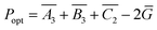 | (15) |
where
Popt denotes the optimal predicted output power and

,

, and

are the mean responses of output power data for factor A at level 3, for factor B at level 3, and for factor C at level 2, respectively. These values can be found in
Table 6.
Ḡ denotes the grand average of all the output power data,
Ḡ = 2.89 W. Using
eqn (11), the predicted value of optimal power can be found to be 4.42 W. Also, using
eqn (9), the confidence interval (CI) at the 85% confidence level for the predicted value of the output power is calculated to be ±1.33. It implies that at the confidence level of 85%, the optimal value of output power lies in the range of 3.10 W to 5.75 W. The confirmation run performed at the optimal setting A
3B
3C
2 shows the actual output power of 4.36 W, which is well within the predicted range. The difference between the actual and the predicted values of the output power is 1.28%. Similarly, the optimal efficiency at the optimal setting A
3B
4C
3 can be predicted. Using
eqn (8), the predicted value of optimal efficiency,
ηopt is found to be 5.88%. At the confidence level of 85%, the range for the predicted efficiency can be found to be between 3.9% and 7.9%. The confirmation simulation at the optimal setting of A
3B
4C
3 shows the efficiency of 6.07%, which is 3.2% higher than the predicted value.
It is important to note that both power and efficiency are maximum at an intermediate value of leg cross-sectional area: 1.5 × 1.5 mm2. The performance of a TE device normally increases with an increase in leg cross-sectional area; however, since the overall area of the TEG module is fixed at 30 × 30 mm2, increasing the cross-sectional area beyond 1.5 × 1.5 mm2 drastically reduces the number of p–n legs, thereby causing both power and efficiency to decrease. Our finding regarding the optimal leg height (1.5 mm for power and 1.75 mm for efficiency) is in agreement with the results shown by other researchers. Rowe33 reported that in order to obtain high efficiency, the TEG module should be designed with long thermocouples. However, if a large power per unit area is needed the thermocouple length should be optimized at a relatively shorter length. Finally, considering the optimal value of load resistance, previous studies have reported that TEGs perform the best when external load resistance equals the effective internal resistance;18 therefore, an intermediate value of load resistance (4.0 Ω for power and 6.0 Ω for efficiency) has appeared as the optimal resistive load. In addition, since the optimal control factors for output power and efficiency are different, it is apparent that the optimum design of a TEG module is likely to be a compromise between obtaining high efficiency or large output power. The difference in output power at the two optimal settings, A3B3C2 and A3B4C3, is only 0.1 W; therefore, we have considered the second setting A3B4C3 as the optimal setting and have fixed the cross-sectional area of 1.50 × 1.50 mm2 and height 1.75 mm for the remainder of the paper. These are nearly the same geometric parameters of the p–n legs as that used in ref. 17.
Full factorial design of optimization and validation of the Taguchi results
In order to validate the Taguchi results, we conducted full-factorial design of optimization, where each of the control factors was varied one-by-one and numerous simulations were performed to determine the optimal performance. Fig. 3(a)–(e) show variation of output power as a function of load resistance at different cross-sectional areas and heights of p–n legs. Fig. 3(f) summarizes the peak output power (at the optimal load) versus leg height at different cross-sectional areas. In the given range of parameters considered in this study, it can be seen that the highest peak output power of 4.36 W occurs at the cross-sectional area of 1.5 × 1.5 mm2, height of 1.5 mm, and resistive load of 4.0 Ω. This is exactly the same optimal setting predicted by the Taguchi method discussed in the last section. Likewise, Fig. 3(h)–(k) show the efficiency versus load resistance at different cross-sectional areas and heights of the p–n legs. Fig. 3(l) summarizes the peak efficiency (at the optimal load) versus the leg height at different cross-sectional areas. The highest efficiency of 6.36% can be found to occur at the cross-sectional area of 1.5 × 1.5 mm2, height of 2.0 mm, and resistive load of 6 Ω. The Taguchi method, however, predicted the optimal efficiency at the cross-sectional area of 1.5 × 1.5 mm2, height of 1.75 mm and load of 6 Ω. It can be seen from Fig. 3(h)–(k) that although this is not the optimal setting, its efficiency (6.07%) is close to the highest value. These results, therefore, confirm that the Taguchi method is very effective tool for predicting the optimal or near optimal geometric parameters of TEGs with far less number of optimization runs than the traditional full-factorial optimization method.
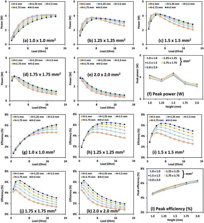 |
| | Fig. 3 The output power and efficiency at different leg geometric parameters and load resistance obtained using the full-factorial design of optimization. H denotes the height of the p–n legs. (a) Output power versus load at a fixed cross-sectional area of 1.0 × 1.0 mm2. (b) Output power versus load at a fixed cross-sectional area of 1.25 × 1.25 mm2. (c) Output power versus load at a fixed cross-sectional area of 1.5 × 1.5 mm2. (d) Output power versus load at a fixed cross-sectional area of 1.75 × 1.75 mm2. (e) Output power versus load at a fixed cross-sectional area of 2.0 × 2.0 mm2. (f) Peak output power at the optimal load versus the leg height at different cross-sectional areas. (g) Efficiency versus load at a fixed cross-sectional area of 1.0 × 1.0 mm2. (h) Efficiency versus load at a fixed cross-sectional area of 1.25 × 1.25 mm2. (i) Efficiency versus load at a fixed cross-sectional area of 1.5 × 1.5 mm2. (j) Efficiency versus load at a fixed cross-sectional area of 1.75 × 1.75 mm2. (k) Efficiency versus load at a fixed cross-sectional area of 2.0 × 2.0 mm2. (l) Peak efficiency (at the optimal load) versus the leg height at different cross-sectional areas. | |
Optimizing the geometric parameters of the heat sink
Table 7 shows the control factors and their levels considered for the optimization of the heat sink using the Taguchi method. The control factors include two geometric parameters (thickness and height) of the aluminium fins and resistive load. Table 8 shows the number of simulation trials and the combination in which the control factors are varied per L25 orthogonal array. The TEG output response: the output power (P) and efficiency (η) obtained by each trial are given in the 5th and 7th columns, respectively. “Larger is better” signal-to-noise ratios, S/NP for power and S/Nη for efficiency are also shown. Tables S3 and S4 in the ESI document† show the mean response for raw data and for S/N data for output power and efficiency. The same data have been plotted in Fig. S2(a) and (b) shown in the ESI document.† Both, the mean of the S/NP ratios and the mean of S/Nη ratios, are found highest when factor A is at level 1, factor B is at level 5, and factor C is at level 3. Therefore, the combination A1B5C3 (fin thickness: 0.5 mm, fin height: 30 mm, and resistive load: 8.0 Ω) is the optimal control factor setting for the highest output power as well as efficiency.
Table 7 Control factors and their levels considered for geometric optimization of the heat sink
| Control factors |
Levels |
| (1) |
(2) |
(3) |
(4) |
(5) |
| (A) |
Fin thickness (mm) |
0.5 |
0.75 |
1.0 |
1.25 |
1.5 |
| (B) |
Fin height (mm) |
10 |
15 |
20 |
25 |
30 |
| (C) |
External resistance (Ω) |
2.0 |
5.0 |
8.0 |
11.0 |
15.0 |
Table 8 Variation of control factors per L25 orthogonal array, power (P), efficiency (η), and the “larger is better” signal-to-noise ratios, S/NP and S/Nη
| Trial |
Control factors |
P (W) |
S/NP (dB) |
η (%) |
S/Nη (dB) |
| (A) |
(B) |
(C) |
| 1 |
1 |
1 |
1 |
0.7160 |
−2.9024 |
1.810 |
−34.844 |
| 2 |
1 |
2 |
2 |
1.4498 |
3.2262 |
3.319 |
−29.581 |
| 3 |
1 |
3 |
3 |
1.7774 |
4.9954 |
3.895 |
−28.189 |
| 4 |
1 |
4 |
4 |
1.8620 |
5.3998 |
4.000 |
−27.959 |
| 5 |
1 |
5 |
5 |
1.7867 |
5.0409 |
3.825 |
−28.348 |
| 6 |
2 |
1 |
2 |
0.8940 |
−0.9732 |
2.548 |
−31.877 |
| 7 |
2 |
2 |
3 |
1.3082 |
2.3333 |
3.299 |
−29.632 |
| 8 |
2 |
3 |
4 |
1.5160 |
3.6141 |
3.594 |
−28.890 |
| 9 |
2 |
4 |
5 |
1.5473 |
3.7916 |
3.561 |
−28.969 |
| 10 |
2 |
5 |
1 |
1.3495 |
2.6033 |
2.594 |
−31.720 |
| 11 |
3 |
1 |
3 |
0.8214 |
−1.7088 |
2.570 |
−31.800 |
| 12 |
3 |
2 |
4 |
1.1209 |
0.9914 |
3.060 |
−30.286 |
| 13 |
3 |
3 |
5 |
1.2558 |
1.9782 |
3.197 |
−29.904 |
| 14 |
3 |
4 |
1 |
1.0909 |
0.7560 |
2.295 |
−32.783 |
| 15 |
3 |
5 |
2 |
1.74793 |
4.8505 |
3.683 |
−28.677 |
| 16 |
4 |
1 |
4 |
0.70524 |
−3.0331 |
2.391 |
−32.428 |
| 17 |
4 |
2 |
5 |
0.9275 |
−0.6538 |
2.728 |
−31.283 |
| 18 |
4 |
3 |
1 |
0.82569 |
−1.6644 |
1.963 |
−34.143 |
| 19 |
4 |
4 |
2 |
1.42423 |
3.0716 |
3.286 |
−29.666 |
| 20 |
4 |
5 |
3 |
1.6497 |
4.3479 |
3.742 |
−28.538 |
| 21 |
5 |
1 |
5 |
0.60036 |
−4.4317 |
2.169 |
−33.276 |
| 22 |
5 |
2 |
1 |
0.57639 |
−4.7857 |
1.603 |
−35.903 |
| 23 |
5 |
3 |
2 |
1.11481 |
0.94403 |
2.875 |
−30.828 |
| 24 |
5 |
4 |
3 |
1.37312 |
2.75417 |
3.386 |
−29.406 |
| 25 |
5 |
5 |
4 |
1.48065 |
3.40903 |
3.549 |
−28.998 |
Table S5 in the ESI document† shows the ANOVA table for the output power data. The percentage contribution from the fin thickness, fin height, and resistive load on output power can be seen to be 19.60%, 60.06%, and 19.40%, respectively. Therefore, the fin height is the most prominent factor that affects the output power followed by the fin thickness and the resistive load. The ANOVA for efficiency is shown in Table S6 in the ESI document.† The percentage contribution from the fin thickness, fin height, and resistive load on efficiency is 11.40%, 37.39%, and 50.52%, respectively. Therefore, the height of the fins and the resistive load are the two most prominent factors, followed by the fin thickness. The contribution by the error term is very small (0.94% for output power and 0.60% for efficiency), indicating the insignificant effect from the external factors that were not included in this study.
Using eqn (8), the predicted value of optimal output power was found to be 2.03 W. In addition, using eqn (9), the confidence interval (CI) at the 85% confidence level for the predicted value of the output power was calculated to be ±0.103. It implies that at the confidence level of 85%, the optimal value of output power lies in the range of 1.93 W to 2.14 W. The confirmation run performed at the optimal setting A1B5C3 shows the output power of 2.1 W, which is well within the predicted range. Also, the difference between the actual and the predicted values of power is about 3.2%. Similarly, the optimal efficiency at the optimal setting A1B5C3 can also be predicted. The predicted value of the optimal efficiency ηopt was found to be 4.23%. The confirmation simulation at the optimal setting of A1B5C3 shows the efficiency of 4.25%, which is 0.6% higher than the predicted value.
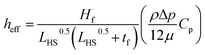
The optimal geometry of the heat sink predicted by the Taguchi method is in agreement with the findings of other researchers. Chen et al.54 obtained an optimal fin height of 28 mm from the range of 7 mm to 28 mm and an optimal fin thickness of 0.1 mm from the range 0.1 to 0.4 mm selected in their study. Clearly, the largest fin height and smallest fin thickness appeared as the optimal geometric dimensions of the heat sink. Likewise, Jang et al.73 reported that an increase of fin height leads to intensification of the heat transfer rate due to the development of new thermal boundary layers, thereby improving both the power and efficiency of TEGs. In addition, increasing the number of fins by decreasing the fin thickness increases the total fin surface area exposed for cooling, which eventually increases the heat transfer rate and improves the TEG performance.73,74 Theoretically, for a heat sink of the fixed base length and width, LHS, fin height Hf, and fin thickness tf, the effective heat transfer coefficient (heff) is expressed as54
| |  | (16) |
Hence, for fixed values of other parameters, the effective heat transfer coefficient (heff) increases with an increase in fin height Hf and with a decrease in fin thickness tf.
Full factorial design of optimization and validating the Taguchi results for the heat sink
Fig. 4(a)–(l) show output power and efficiency versus load resistance at different thicknesses and heights of the fins. In the given range of parameters considered in this study, it can be seen from Fig. 4(a)–(f) that the highest output power of 2.10 W occurs at the fin thickness of 0.5 mm, fin height of 30 mm, and resistive load of 8.0 Ω. Similarly, Fig. 4(g)–(l) show that the highest efficiency of 4.25% occurs at the fin thickness of 0.5 mm, fin height of 30 mm, and resistive load of 8.0 Ω. These are the same optimal setting predicted by the Taguchi method discussed in the last section. These results confirm that the Taguchi method can successfully predict the optimal geometric parameters of the heat sink.
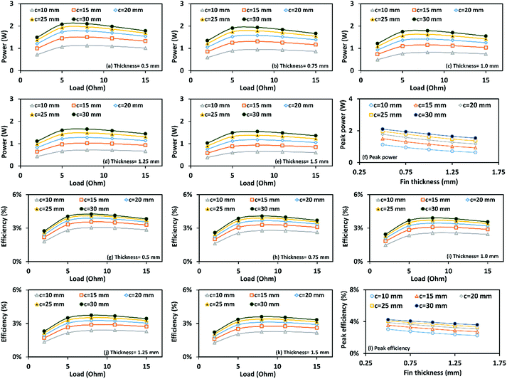 |
| | Fig. 4 The output power and efficiency at different geometric parameters of the heat sink and the load resistance obtained using the full-factorial design of optimization, where c denotes the fin height. (a) Output power versus load at a fixed fin thickness of 0.5 mm. (b) Output power versus load at a fixed fin thickness of 0.75 mm. (c) Output power versus load at a fixed fin thickness of 1.0 mm. (d) Output power versus load at a fixed fin thickness of 1.25 mm. (e) Output power versus load at a fixed fin thickness of 1.5 mm. (f) Peak output power (at the optimal load) versus fin thickness at different fin heights. (g) Efficiency versus load at a fixed fin thickness of 0.5 mm. (h) Efficiency versus load at a fixed fin thickness of 0.75 mm. (i) Efficiency versus load at a fixed fin thickness of 1.0 mm. (j) Efficiency versus load at a fixed fin thickness of 1.25 mm. (k) Efficiency versus load at a fixed fin thickness of 1.5 mm. (l) Peak efficiency (at the optimal load) versus fin thickness at different fin heights. | |
Effect of operating conditions: the heat transfer coefficient and the ambient temperature
In Section 4.2, when the geometric parameters of the p–n legs were optimized, we noted that the optimized TEG had the maximum output power of 4.36 W and the maximum efficiency of 6.07%. However, in Section 4.4, when the geometric parameters of the heat sink were optimized, the optimal output power reduced to 2.10 W, which is less than half of the value found earlier. Similarly, the optimal efficiency also reduced to 4.25%. This happened because of the difference in the boundary conditions between the two cases. In the first case, hot-side and cold-side temperatures were fixed at 513 K and 295 K, respectively; whereas, in the second case, only the hot-side temperature was fixed at 513 K. The cold-side had a heat sink and the heat-sink was allowed to cool under ambient conditions at a temperature of 295 K with a total heat transfer film coefficient of 20 W m−2 K−1. The heat sink temperature on the cold-side would always remain higher than the ambient temperature. The second case, therefore, can be considered more realistic. This implies that, in practice, a TEG designed for a rated efficiency of 6.07% would have a maximum practical efficiency of only 4.27%. The efficiency of the TEG, however, can be enhanced by forced cooling. Fig. 5(a) and (b) show the variation in output power and efficiency versus load resistance for different heat transfer coefficients, h∞, in the range of 10–60 W m−2 K−1. Increasing the heat transfer coefficient from 10 to 60 W m−2 K−1 increases the optimal output power from 1.43 W to 2.83 W and efficiency from 3.46% to 4.92% at a fixed ambient temperature of 295 K. It can be observed from Fig. 5(e) and (f) that a higher value of h∞ leads to lower heat-sink average temperature on the cold-side, resulting in better performance by the TEG. The performance of the TEG, however, reduces with an increase in the ambient temperature. Fig. 5(c) and (d) depict the variation in output power and efficiency versus load resistance for different ambient temperatures, T∞, in the range of 273–313 K. Increasing the ambient temperature from 273 K to 313 K decreases the optimal output power from 2.56 W to 1.56 W and efficiency from 4.71% to 3.63% at a fixed heat transfer coefficient of 20 W m−2 K−1. It can be noted from Fig. 5(g) and (h) that the ambient temperature of 273 K (at h∞ = 20 W m−2 K−1) has almost the same effect on the heat sink temperature as the heat transfer coefficient of 60 W m−2 K−1 (at T∞ = 295 K). Increasing the ambient temperature increases the cold-side temperature, resulting in deterioration in the performance of the TEG.
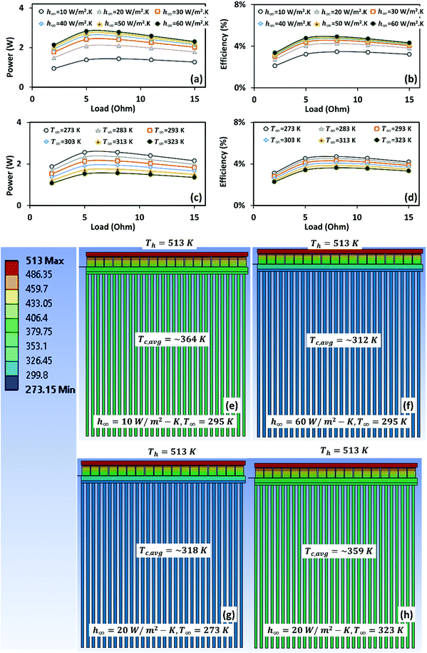 |
| | Fig. 5 Effect of operating conditions on the performance of a TEG. (a) Output power versus resistive load at different heat transfer coefficients. (b) Efficiency versus resistive load at different heat transfer coefficients. (c) Output power versus resistive load at different ambient temperatures. (d) Efficiency versus resistive load at different ambient temperatures. The ambient temperature is fixed at 295 K in (a) and (b). The heat transfer coefficient is fixed at 20 W m−2 K−1 in (c) and (d). Temperature contours of the TEG and heat sink under different operating conditions. Tc,avg denotes the average temperature of the heat sink. (e) and (f) Increasing the heat transfer coefficient decreases the cold-side temperature, resulting in better performance of the TEG. (g) and (h) Increasing the ambient temperature increases the cold-side temperature, resulting in poorer performance by the TEG. | |
It is important to note that in this study, we have considered fixed electrical and thermal contact resistances as 1.0 × 10⁻⁹ Ω m2 and 2.2 × 10⁻⁴ m2 K W−1, respectively, to reduce the number of invariants. In practice, however, it is very difficult to maintain a constant value of contact resistances due to their inherent nature. Contact resistance depends on numerous factors such as contact pressure, interfacial materials, surface deformations, surface roughness and quality of deposition. Therefore, contact quality between two interfaces depends not only on the material properties of the interfacial layer but also on the manufacturing techniques and operating conditions. Several studies75–78 in the past have attempted to enhance the performance of thermoelectric devices by reducing contact resistances using various evaluation and fabrication techniques. However, such attempts are limited and often concentrated to certain thermoelectric materials. The effect of contact resistances becomes more prominent in the case of a segmented thermoelectric generator. Finding the compatibility relationship among various thermoelectric materials, the diffusion barriers and the matching interface layers is a potential area of future research in the design of high efficiency thermoelectric generators.
Conclusions
A comprehensive optimization study on BiTe-based thermoelectric generators using the Taguchi method is conducted. The Taguchi optimization method enables achieving the optimal control parameters with a much smaller number of trials than the conventional optimization techniques, where only one factor is changed at a time. The optimization of a 30 × 30 mm2 TEG module was achieved in four consecutive stages. In the first stage, we validated the numerical model with the published experimental data. In the second stage, the geometric parameters of p–n legs were optimized using the Taguchi method. The full-factorial design of optimization was also performed and the results obtained from the Taguchi method were validated. In the third stage, we optimized the heat sink geometry using the Taguchi method and validated the Taguchi results with the results obtained from the full-factorial design of optimization. In the fourth and last step, we studied the effect of operating conditions, viz. the total heat transfer coefficient and the ambient temperature on the performance of TEGs. The major findings of the paper are summarized below:
• Under different levels of geometric parameters examined, it was found that p–n legs having a cross-sectional area of 1.5 × 1.5 mm2 and height of 1.5 mm provided the highest output power.
• The p–n legs having a cross-sectional area of 1.5 × 1.5 mm2 and height of 1.75 mm were found to provide the highest efficiency.
• Under different levels of fin dimensions examined, it was found that the performance of a TEG is highest when the fin thickness is 0.5 mm and fin height is 30 mm.
• The study also showed that a TEG designed under ideal laboratory conditions is expected to have much lower performance under actual operating conditions. For example, a TEG designed at a fixed hot-side temperature of 513 K and cold-side temperature of 295 K was found to have a maximum efficiency of about 6%. However, the efficiency of the TEG reduced to 4.25% when it was operated under an ambient condition of 295 K.
• The output power of the TEG was found to increase from 1.43 W to 2.83 W and efficiency from 3.46% to 4.92% on increasing the heat transfer coefficient from 10 to 60 W m−2 K−1 at a fixed ambient temperature of 295 K.
• The output power of the TEG was found to reduce from 2.56 W to 1.56 W and efficiency from 4.71% to 3.63% on increasing the ambient temperature from 273 K to 313 K at a fixed heat transfer coefficient of 20 W m−2 K−1.
Conflicts of interest
There are no conflicts to declare.
Acknowledgements
R. K. acknowledges the financial support from the ICTAS Doctoral Scholars Program and AMRDEC through the SBIR program (W31P4Q-16-C-0083). S. P. acknowledges the financial support through the DARPA MATRIX program (W911NF-16-2-0010). P. K. would like to thank Office of Naval Research (ONR) for supporting his research (N00014-16-1-3043).
References
- C. Forman, I. K. Muritala, R. Pardemann and B. Meyer, Renew. Sustain. Energy Rev., 2016, 57, 1568–1579 CrossRef.
- K. Semkov, E. Mooney, M. Connolly and C. Adley, Appl. Therm. Eng., 2014, 70, 716–722 CrossRef CAS.
-
I. Johnson, W. T. Choate and A. Davidson, Waste Heat Recovery. Technology and Opportunities in US Industry, BCS, Inc., Laurel, MD (United States), 2008 Search PubMed.
- G.-D. Zhan, J. D. Kuntz, A. K. Mukherjee, P. Zhu and K. Koumoto, Scr. Mater., 2006, 54, 77–82 CrossRef CAS.
- M. H. Elsheikh, D. A. Shnawah, M. F. M. Sabri, S. B. M. Said, M. H. Hassan, M. B. A. Bashir and M. Mohamad, Renew. Sustain. Energy Rev., 2014, 30, 337–355 CrossRef.
- K. Cai, E. Mueller, C. Drasar and C. Stiewe, Solid State Comm., 2004, 131, 325–329 CrossRef CAS.
- X. Zheng, C. Liu, Y. Yan and Q. Wang, Renew. Sustain. Energy Rev., 2014, 32, 486–503 CrossRef CAS.
- L. Hu, H. Wu, T. Zhu, C. Fu, J. He, P. Ying and X. Zhao, Adv. Energy Mater., 2015, 5(17) DOI:10.1002/aenm.201500411.
- L.-P. Hu, T.-J. Zhu, Y.-G. Wang, H.-H. Xie, Z.-J. Xu and X.-B. Zhao, NPG Asia Mater., 2014, 6, e88 CrossRef CAS.
- S. I. Kim, K. H. Lee, H. A. Mun, H. S. Kim, S. W. Hwang, J. W. Roh, D. J. Yang, W. H. Shin, X. S. Li and Y. H. Lee, Science, 2015, 348, 109–114 CrossRef CAS PubMed.
- B. Poudel, Q. Hao, Y. Ma, Y. Lan, A. Minnich, B. Yu, X. Yan, D. Wang, A. Muto and D. Vashaee, Science, 2008, 320, 634–638 CrossRef CAS PubMed.
- J.-J. Shen, T.-J. Zhu, X.-B. Zhao, S.-N. Zhang, S.-H. Yang and Z.-Z. Yin, Energy Environ. Sci., 2010, 3, 1519–1523 CAS.
- X. Tang, W. Xie, H. Li, W. Zhao, Q. Zhang and M. Niino, Appl. Phys. Lett., 2007, 90, 12102 CrossRef.
- J. Cui, H. Xue and W. Xiu, Mater. Lett., 2006, 60, 3669–3672 CrossRef CAS.
- L. Hu, T. Zhu, X. Yue, X. Liu, Y. Wang, Z. Xu and X. Zhao, Acta Mater., 2015, 85, 270–278 CrossRef CAS.
- T. Zhang, J. Jiang, Y. Xiao, Y. Zhai, S. Yang and G. Xu, J. Mater. Chem. A, 2013, 1, 966–969 CAS.
- F. Hao, P. Qiu, Y. Tang, S. Bai, T. Xing, H.-S. Chu, Q. Zhang, P. Lu, T. Zhang and D. Ren, Energy Environ. Sci., 2016, 9, 3120–3127 CAS.
- X. Niu, J. Yu and S. Wang, J. Power Sources, 2009, 188, 621–626 CrossRef CAS.
- C.-T. Hsu, G.-Y. Huang, H.-S. Chu, B. Yu and D.-J. Yao, Appl. Energy, 2011, 88, 1291–1297 CrossRef.
- X. Gou, H. Xiao and S. Yang, Appl. Energy, 2010, 87, 3131–3136 CrossRef.
- D. Rowe and G. Min, IEE Proc. Sci. Meas. Technol., 1996, 143, 351–356 CrossRef.
- D. Mitrani, J. Salazar, A. Turó, M. J. García and J. A. Chávez, Microelectron. J., 2009, 40, 1398–1405 CrossRef CAS.
- X.-D. Wang, Y.-X. Huang, C.-H. Cheng, D. T.-W. Lin and C.-H. Kang, Energy, 2012, 47, 488–497 CrossRef CAS.
- J. Pérez–Aparicio, R. Palma and R. Taylor, Int. J. Heat Mass Transfer, 2012, 55, 1363–1374 CrossRef.
- C.-H. Cheng, S.-Y. Huang and T.-C. Cheng, Int. J. Heat Mass Transfer, 2010, 53, 2001–2011 CrossRef CAS.
- J.-H. Meng, X.-D. Wang and X.-X. Zhang, Appl. Energy, 2013, 108, 340–348 CrossRef.
- K. Yazawa and A. Shakouri, J. Appl. Phys., 2012, 111, 024509 CrossRef.
- P. Mayer and R. Ram, Nanoscale Microscale Thermophys. Eng., 2006, 10, 143–155 CrossRef.
- L. Chen, J. Gong, F. Sun and C. Wu, Int. J. Therm. Sci., 2002, 41, 95–99 CrossRef.
- A. Z. Sahin and B. S. Yilbas, Energy Convers. Manage., 2013, 65, 26–32 CrossRef.
- R. Yang, G. Chen, G. J. Snyder and J.-P. Fleurial, J. Appl. Phys., 2004, 95, 8226–8232 CrossRef CAS.
- B. Yilbas and A. Sahin, Energy, 2010, 35, 5380–5384 CrossRef.
-
D. M. Rowe, Thermoelectrics Handbook: Macro to Nano, CRC press, 2005 Search PubMed.
- B. Jang, S. Han and J.-Y. Kim, Microelectron. Eng., 2011, 88, 775–778 CrossRef CAS.
- Z. Ouyang and D. Li, Sci. Rep., 2016, 6, 24123 CrossRef CAS PubMed.
- C.-C. Wang, C.-I. Hung and W.-H. Chen, Energy, 2012, 39, 236–245 CrossRef CAS.
- J. Luo, L. Chen, F. Sun and C. Wu, Energy Convers. Manag., 2003, 44, 3197–3206 CrossRef.
- L. Chen, J. Li, F. Sun and C. Wu, Appl. Energy, 2005, 82, 300–312 CrossRef CAS.
- G. Fraisse, M. Lazard, C. Goupil and J. Serrat, Int. J. Heat Mass Transfer, 2010, 53, 3503–3512 CrossRef CAS.
- Y.-H. Cheng and W.-K. Lin, Appl. Therm. Eng., 2005, 25, 2983–2997 CrossRef CAS.
- H. Lee, Appl. Energy, 2013, 106, 79–88 CrossRef.
- M. Yamanashi, J. Appl. Phys., 1996, 80, 5494–5502 CrossRef CAS.
- Y.-X. Huang, X.-D. Wang, C.-H. Cheng and D. T.-W. Lin, Energy, 2013, 59, 689–697 CrossRef.
- M. Nalbant, H. Gökkaya and G. Sur, Mater. Des., 2007, 28, 1379–1385 CrossRef CAS.
- J. A. Ghani, I. Choudhury and H. Hassan, J. Mater. Process. Technol., 2004, 145, 84–92 CrossRef CAS.
- R. Kishore, R. Tiwari, A. Dvivedi and I. Singh, Mater. Des., 2009, 30, 2186–2190 CrossRef CAS.
-
R. Kishore, R. Tiwari and I. Singh, Advances in Production Engineering and Manangement, 2009, vol. 4, pp. 37–46 Search PubMed.
- K. Comakli, F. Simsek, O. Comakli and B. Sahin, Appl. Energy, 2009, 86, 2451–2458 CrossRef CAS.
- K.-T. Chiang, Int. Comm. Heat Mass Tran., 2005, 32, 1193–1201 CrossRef CAS.
- M. Zeng, L. Tang, M. Lin and Q. Wang, Appl. Therm. Eng., 2010, 30, 1775–1783 CrossRef.
- N. Daneshvar, A. Khataee, M. Rasoulifard and M. Pourhassan, J. Hazard. Mater., 2007, 143, 214–219 CrossRef CAS PubMed.
- R. S. Rao, C. G. Kumar, R. S. Prakasham and P. J. Hobbs, Biotechnol. J., 2008, 3, 510–523 CrossRef CAS PubMed.
- B. D. Cobb and J. M. CIarkson, Nucleic Acids Res., 1994, 22, 3801–3805 CrossRef CAS PubMed.
- W.-H. Chen, S.-R. Huang and Y.-L. Lin, Appl. Energy, 2015, 158, 44–54 CrossRef.
- H. Kim, Y. Lee and K. H. Lee, Int. J. Precis. Eng. Manuf., 2012, 13, 261–267 CrossRef.
- R. Anant Kishore, P. Kumar, M. Sanghadasa and S. Priya, J. Appl. Phys., 2017, 122, 025109 CrossRef.
- A. Montecucco, J. Buckle and A. Knox, Appl. Therm. Eng., 2012, 35, 177–184 CrossRef.
- F. Völklein, G. Min and D. Rowe, Sens. Actuators, A, 1999, 75, 95–101 CrossRef.
- B. Huang and C. Duang, Int. J. Refrig., 2000, 23, 197–207 CrossRef.
- M. Chen, L. A. Rosendahl and T. Condra, Int. J. Heat Mass Transfer, 2011, 54, 345–355 CrossRef.
- K. H. Lee and O. J. Kim, Int. J. Heat Mass Transfer, 2007, 50, 1982–1992 CrossRef.
- W. Zhu, Y. Deng, Y. Wang and A. Wang, Microelectron. J., 2013, 44, 860–868 CrossRef.
-
ANSYS mechanical APDL theory reference (release 15.0), ANSYS Inc., 2013 Search PubMed.
- O. Mengali and M. Seiler, Adv. Energy Convers., 1962, 2, 59–68 CrossRef CAS.
- O. Högblom and R. Andersson, J. Electron. Mater., 2014, 43, 2247–2254 CrossRef.
- W.-H. Chen, C.-C. Wang and C.-I. Hung, Energy Convers. Manage., 2014, 87, 566–575 CrossRef.
- D. Astrain, J. Vián, A. Martinez and A. Rodríguez, Energy, 2010, 35, 602–610 CrossRef.
-
G. Taguchi and G. Taguchi, System of Experimental Design; Engineering Methods to Optimize Quality and Minimize Costs, 1987 Search PubMed.
-
A. Mitra, Fundamentals of Quality Control and Improvement, John Wiley & Sons, 2016 Search PubMed.
- Minitab 17 Supporting Topics, http://https://support.minitab.com/en-us/minitab/18/help-and-how-to/modeling-statistics/doe/supporting-topics/taguchi-designs/what-is-the-signal-to-noise-ratio/, accessed on Oct 23, 2017.
- M. Yousefieh, M. Shamanian and A. Saatchi, J. Mater. Eng. Perform., 2012, 21, 1978–1988 CrossRef CAS.
-
M. Yovanovich, J. Culham and P. Teertstra, Electronics Cooling, 1997, vol. 3, pp. 24–29 Search PubMed.
- J.-Y. Jang, Y.-C. Tsai and C.-W. Wu, Energy, 2013, 53, 270–281 CrossRef.
- T. Y. Kim, S. Lee and J. Lee, Energy Convers. Manage., 2016, 124, 470–479 CrossRef.
- P. H. Ngan, N. Van Nong, L. T. Hung, B. Balke, L. Han, E. M. J. Hedegaard, S. Linderoth and N. Pryds, J. Electron. Mater., 2016, 45, 594–601 CrossRef CAS.
- R. Bjørk, J. Electron. Mater., 2016, 45, 1301–1308 CrossRef.
- Y. Kim, G. Yoon and S. Park, Exp. Mech., 2016, 56, 861–869 CrossRef CAS.
- D. Ebling, K. Bartholomé, M. Bartel and M. Jägle, J. Electron. Mater., 2010, 39, 1376–1380 CrossRef CAS.
Footnote |
| † Electronic supplementary information (ESI) available. See DOI: 10.1039/c7se00437k |
|
| This journal is © The Royal Society of Chemistry 2018 |

 ,
Prashant
Kumar
,
Prashant
Kumar


 represent the heat flux, electric current density, electric field, and thermal gradient, respectively. The Seebeck coefficient α and Peltier coefficient π are related as π = Tα. We have used commercial finite element analysis (FEA) code ANSYS v17.0 (ANSYS Inc., USA) to numerically solve the thermoelectric constitutive equations. ANSYS deduces the thermoelectric constitutive eqn (8) and (9) in the form of a finite element matrix equation of thermoelectricity given as63


 (dB)
(dB) (dB)
(dB)
 ,
,  , and
, and  are the mean responses of output power data for factor A at level 3, for factor B at level 3, and for factor C at level 2, respectively. These values can be found in Table 6. Ḡ denotes the grand average of all the output power data, Ḡ = 2.89 W. Using eqn (11), the predicted value of optimal power can be found to be 4.42 W. Also, using eqn (9), the confidence interval (CI) at the 85% confidence level for the predicted value of the output power is calculated to be ±1.33. It implies that at the confidence level of 85%, the optimal value of output power lies in the range of 3.10 W to 5.75 W. The confirmation run performed at the optimal setting A3B3C2 shows the actual output power of 4.36 W, which is well within the predicted range. The difference between the actual and the predicted values of the output power is 1.28%. Similarly, the optimal efficiency at the optimal setting A3B4C3 can be predicted. Using eqn (8), the predicted value of optimal efficiency, ηopt is found to be 5.88%. At the confidence level of 85%, the range for the predicted efficiency can be found to be between 3.9% and 7.9%. The confirmation simulation at the optimal setting of A3B4C3 shows the efficiency of 6.07%, which is 3.2% higher than the predicted value.


