DOI:
10.1039/C8RA01393D
(Paper)
RSC Adv., 2018,
8, 20941-20951
Visual synchronization of two 3-variable Lotka–Volterra oscillators based on DNA strand displacement
Received
13th February 2018
, Accepted 21st May 2018
First published on 7th June 2018
Abstract
DNA strand displacement as a theoretic foundation is helpful in constructing reaction networks and DNA circuits. Research on chemical kinetics is significant to exploit the inherent potential property of biomolecular systems. In this study, we investigated two typical reactions and designed DNA strands with a fluorophore and dark quencher for reaction networks using a 3-variable Lotka–Volterra oscillator system as an example to show the convenience of and superiority for observation of dynamic trajectory using our design, and took advantage of the synchronization reaction module to synchronize two 3-variable Lotka–Volterra oscillators. The classical theory of chemical reaction networks can be used to represent biological processes for mathematical modeling. We used this method to simulate the nonlinear kinetics of a 3-variable Lotka–Volterra oscillator system.
1. Introduction
Nonlinear kinetics exists widely in mass chemical reaction equations. Chemical reactions with DNA strand displacement (DSD) also have the property of being nonlinear and cascading. We can use the property of cascading to construct complex chemical reaction networks (CRNs) as well as to compile chemical equations into circuit systems, for example, in pulse counter and incrementer state machines.1–3
With the aid of DNA strand displacement, massive DNA circuits, including digital and analog circuits, have been designed and validated by experiments.4–13 The outputs of the DNA circuit are represented by the concentrations of the DNA strands, but the detection of concentration is difficult or even impossible in some cases. For example, the structure of a DNA polymer is massive, complex, and unstable, such that detection of the concentration of the DNA polymer is impossible.14 If the DNA strand is designed with a fluorophore and dark quencher, observation of the output is convenient and fast. Luminous intensity is enhanced with an increase in the concentration of DNA strands.15 Thus, it is helpful to measure the concentration of DNA strands by fluorescence intensity. This property is particularly useful for digital circuits because these circuits are encoded with binary bits, where 2 possible values of each bit are “0” and “1”. If the luminous intensity is strong enough, the value of the output is “1”, otherwise the value of the output is “0”. For an analog circuit, the output is represented qualitatively by luminous intensity; for polymerization of a hybridization chain reaction,14 characterization of the hyperbranched chain reaction can be recognized by fluorescence intensity.
Synchronization is an important dynamical behavior and a general and ubiquitous phenomenon that has been investigated in a variety of fields such as complex networks, chemical reaction networks,16–18 secure communication, and genetic regulatory networks. Recently, it was found that synchronization is beneficial to DNA nanotechnology; for example, synchronization is applied in self-assembly,19 gene expression20 and DNA replication.21 Synchronized systems can enjoy common dynamical behavior and isochronous signal transition or transmission. Thus, synchronization has extensive application potential in digital and analog DNA circuits.
As compared to previous studies, we have proposed catalysis, degradation and synchronization reaction modules with a fluorophore and dark quencher, and identified different DNA strands with different colors of fluorophores, where the synchronization reaction module is a new reaction module. Then, we compiled these reaction modules into the 3-variable Lotka–Volterra oscillator and realized synchronization of two 3-variable Lotka–Volterra oscillator systems. From the simulations of these reaction modules, it was demonstrated that the DNA implementation of CRN can imitate the dynamical behavior of an ideal formal reaction, and there is a relationship between the reaction rates of DNA CRNs, intermediate CRNs and ideal formal CRNs.
We used visual DSD software to design the DNA strand and test the feasibility of the chemical reaction with DNA strand displacement, and utilized chemical reaction network (CRN) software to numerically simulate the dynamic behavior of the 3-variable Lotka–Volterra oscillator.
2. Recent work
2.1. DNA strand displacement with fluorophore and dark quencher
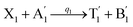
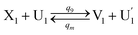
We presented a reversible, bimolecular chemical reaction, as shown in Fig. 1, where A1 and A2 are reactants and A3 and A4 are products; k1 denotes the forward reaction rate, and k2 denotes the backward reaction rate. The reaction begins with an invader strand A1 binding to the target strand A2 based on the Watson-Crick model.22 The position, number, and length determine the feasibility, reversibility, and reaction rate of DNA strand displacement, respectively. The reaction rate first increases and then decreases with an increase in the length of the toehold,23 such that we can adjust the reaction rate by changing the length of the toehold. Reversible and irreversible reactions are 2 types of DNA strand displacement reactions.
 |
| | Fig. 1 DNA strand displacement with the fluorophore and quencher. The arrow in a DNA strand indicates the 3′ end. The domain a2 is 12 nucleotides, and the toehold domain is usually less than 10 nucleotides, so the toehold binding reaction is reversible. | |
The fluorophore and quencher exist at the end of the strand. When the fluorophore and quencher appear in pairs, the fluorophore strand does not fluoresce, but when the fluorophore strand releases from the dark quencher strand, it can be detected by fluorescence intensity.
2.2. DNA strand displacement with hairpin structure
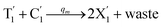
Hairpin24–26 is a special structure for single strand DNA (ssDNA), which can protect some domains. As shown in Fig. 2, domains a2, b1, and b2 are protected before the hairpin is open. When an invader DNA strand X reacts with H, the hairpin is open and then, domains a2, b1, and b2 can be used for further reactions.
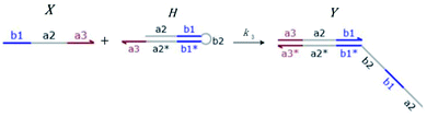 |
| | Fig. 2 DNA strand displacement with a hairpin structure. The toehold b1 is as long as the other toeholds. The hairpin cannot open spontaneously as a result of the dissociation of  hybridization at the end of the branch migration, the loop portion a2 – b1 – b2 of the hairpin is protected if it does not open. hybridization at the end of the branch migration, the loop portion a2 – b1 – b2 of the hairpin is protected if it does not open. | |
3. Results
3.1. CRN modules
In DNA strand displacement as a type of chemical reaction, there is a corresponding relationship between DNA CRNs and the ideal formal CRNs, where there are intermediate CRNs is the transition between DNAs and ideal formal CRNs. In order to endue CRNs modularity, we propose three types of reaction modules by DNA CRNs and ideal CRNs, where [X]0, [XM]0 and [X1]0 represent the initial concentration of species X, XM and X1 in DNA CRNs, intermediate CRNs and ideal CRNs, respectively, and satisfied [X]0 = [XM]0 = [X1]0. [Y]0, [YM]0 and [Y1]0 represent the initial concentration of species Y, YM and Y1 in DNA CRNs, intermediate CRNs and ideal CRNs, respectively, and satisfied [Y]0 = [YM]0 = [Y1]0.
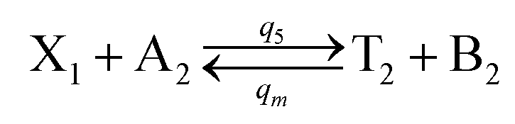
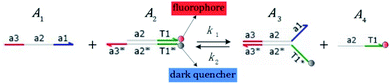
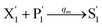
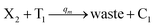
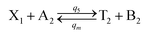
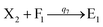
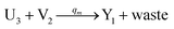
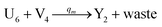
In the catalysis reaction module (1), as shown in Fig. 3(b),  is produced by XM in (5), and the increase in
  will catalyze (6), while the producer XM can catalyze the production of
  . According to (1), d[X]t/dt = −qiCm[X]t and d[XM]t/dt = −θ1[XM]t by (5); if DSD (1) and (2) can approximate to the intermediate (5), qi = θ1/Cm is obtained. According to (3), d[X′]t/dt = −qmCm[X′]t, while
 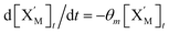 based on (6). If DSD (3) and (4) can approximate to the intermediate (6), qm = θm/Cm. d[X]t/dt = −θ2[X]t and d[XM]t/dt = −qjCm [XM]t, according to (4) and (6); if (4) is equivalent to (6), qj = θ2/Cm. Similarly, we can obtain k1 = θ1 based on (5), (6) and (7). Initial concentrations of the auxiliary species
  and
and  are set to Cm, where [X]0 ≪ Cm, and [X]0, [Y]0 are the initial concentrations of X and Y. As shown in Fig. 3(c), the evolutions of X in DNA CRNs, intermediate CRNs and ideal CRNs are approximately coincident. This shows that DNA CRNs, intermediate CRNs and ideal formal CRNs in the catalysis reaction module (1) are equivalent, but there are nuances between DNA CRNs, intermediate CRNs and ideal formal CRNs.
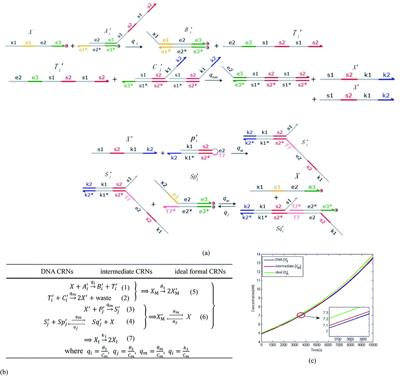 |
| | Fig. 3 Catalysis reaction module (1) X → 2X. DNA reactions are listed in (a); (b) exhibits the DNA CRNs and appropriate ideal CRNs, where intermediate CRNs is the transition between DNAs and ideal formal CRNs; (c) shows the result of the variable X in DNA CRNs, media CRNs and ideal formal CRNs respectively, where Cm = 104 nM and [X]0 = [XM]0 = [XI]0 = 5 nM; qi = 10−8 nM s−1, qj = 10−7 nM s−1 and qm = 10−5 nM s−1. DNA implementation of formal species X′ is gained by species X. Species X reacts with  to displace to displace  in (1), in (1),  releases two X′ in (2). In (3), species X′ reacts with hairpin releases two X′ in (2). In (3), species X′ reacts with hairpin  to produce to produce  , and , and  and releases X in (4) on reaction with and releases X in (4) on reaction with  . This reaction replaces the ssDNA strand without the fluorophore to the ssDNA strand with the fluorophore, as adapted from.4 qm represents a maximum strand displacement rate constant under the assumption of equal binding strength for all full toeholds; when qi and ki are satisfied qi,qj ≪ qm, ki ≪ qmCm; [X]0 and Cm are satisfied [X]0 ≪ Cm, as adapted from.1 . This reaction replaces the ssDNA strand without the fluorophore to the ssDNA strand with the fluorophore, as adapted from.4 qm represents a maximum strand displacement rate constant under the assumption of equal binding strength for all full toeholds; when qi and ki are satisfied qi,qj ≪ qm, ki ≪ qmCm; [X]0 and Cm are satisfied [X]0 ≪ Cm, as adapted from.1 | |
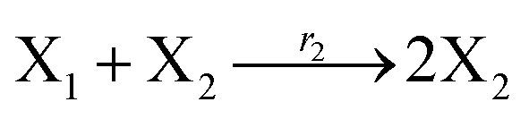
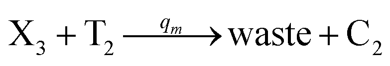
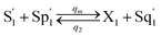
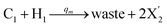
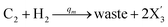
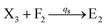
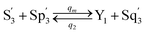
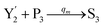
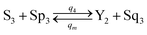
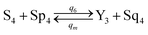
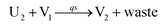
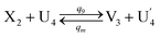
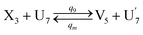
In catalysis reaction module (2), as shown in Fig. 4(b),  is produced by XM and YM in (13), and the increase in
  will catalyze (14), while the producer YM can catalyze the production of
  and consumption of XM. According to ref. 1, we have. qi = θ3. Similar to catalysis reaction module (1), qj = θ4/Cm, qm = θm/Cm and k2 = θ3. Initial concentrations of the auxiliary species Ai, Bi, Hi, Pj, Spj, and Sqj are set to Cm, where [X]0, [Y]0 ≪ Cm. As shown in Fig. 4(c), the evolutions of Y in DNA CRNs, intermediate CRNs and ideal CRNs are approximately coincident. This indicates that DNA CRNs, intermediate CRNs and ideal CRNs in catalysis reaction module (2) are equivalent, but there are nuances between DNA CRNs, intermediate CRNs and ideal CRNs.
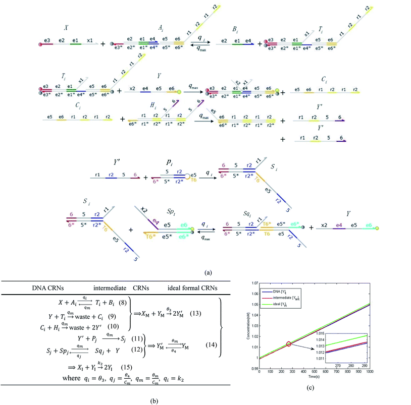 |
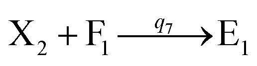
| | Fig. 4 Catalysis reaction module (2) X + Y → 2Y. DNA reactions are listed in (a) and (b) exhibits the DNA CRNs and corresponding ideal formal CRNs, where intermediate CRNs is the transition between DNAs and ideal CRNs; (c) shows the result of the variable Y in DNA CRNs, media CRNs and ideal formal CRNs, respectively, where Cm = 104 nM, [X]0 = [XM]0 = [XI]0 = 5 nM, and [Y]0 = [YM]0 = [YI]0 = 1 nM; qi = 10−5 nM s−1, qj = 10−6 nM s−1 and qm = 10−3 nM s−1. DNA implementation of formal species  is gained by species XM and YM in intermediate CRN (13). Species X reacts with Ai to displace Ti. In (9), Ci is produced when Y irreversibly displaces Ti, and Hi releases 2 Y′ in reaction (10), as adapted from.1 In (11), species Y′ reacts with hairpin Pj to produce Sj, and Sj releases X in (12) on reacting with Spj, as adapted from.4 is gained by species XM and YM in intermediate CRN (13). Species X reacts with Ai to displace Ti. In (9), Ci is produced when Y irreversibly displaces Ti, and Hi releases 2 Y′ in reaction (10), as adapted from.1 In (11), species Y′ reacts with hairpin Pj to produce Sj, and Sj releases X in (12) on reacting with Spj, as adapted from.4 | |
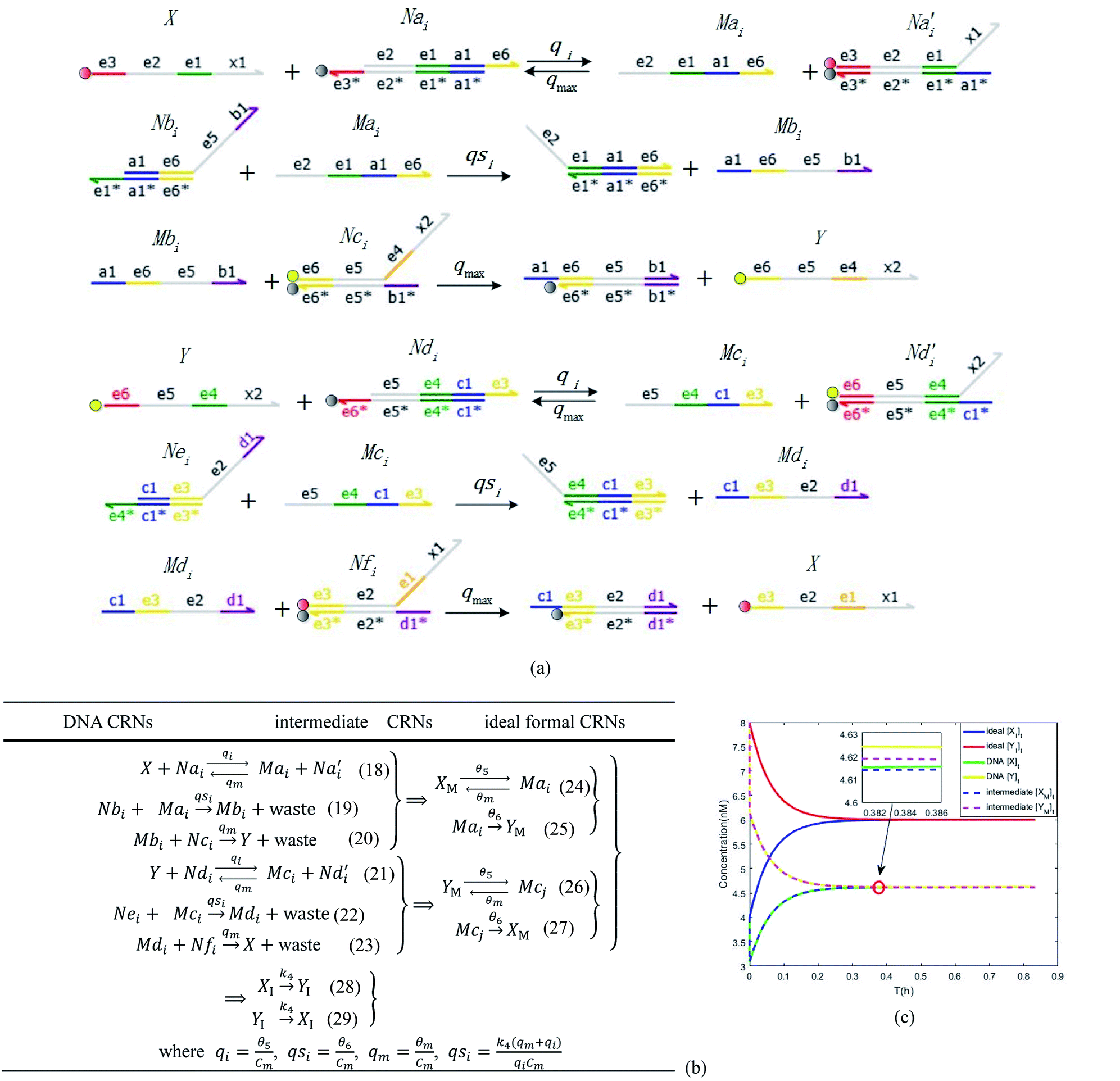
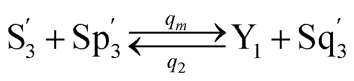
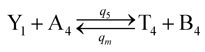
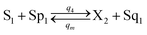
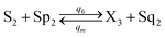
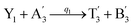
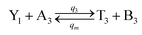
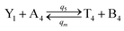
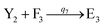
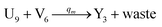
In the synchronization reaction module, it is assumed that X and Mai attain instant equilibrium through (18), with [X]t/[Mai]t = qm/qi; when XM and Mai attain instant equilibrium through (24), we obtain [XM]t/[Mai]t = θ5/θm. According to (19) and (25), we have d[Mai]t/dt = −Cmqsi[Mai]t = −θ6[Mai]t; as a result, qsi = θ6/Cm. Taking (25) and (28) into account, we obtain d[YM]t/dt = θ6[Mai]t and d[YI]t/dt = k4[XI]t, respectively; if intermediate reaction (25) can be approximated to the ideal formal reaction (28), θ6[Mai]t = k4[XI]t. Because [X]t/[Mai]t = qm/qi when X and Mai attain instant equilibrium and [XI]t = [X]t+[Mai]t, we can obtain k4 = qiθ6/(qm + qi) = qsiqiCm/(qm + qi). The initial concentrations of the auxiliary species Nai,  , Nbi, Nci, Ndi,
  , Nei, and Nfi are set to Cm, where [X]0,[Y]0 ≪ Cm. Fig. 6(c) shows that X and Y can share the same dynamic behavior in DNA CRNs, intermediate CRNs and ideal formal CRNs, but their synchronous values are different. The reasons for this phenomenon are as follows:
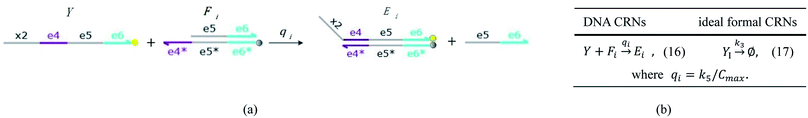 |
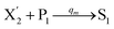
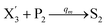
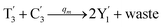
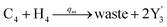
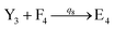
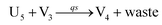
| | Fig. 5 Degradation reaction module Y → ∅: DNA implementation of formal species Y and degradation with auxiliary species Fi; in (16), species Y reacts with species Fi producing inert waste, where the initial concentration of auxiliary species Fi is set to Cm. | |
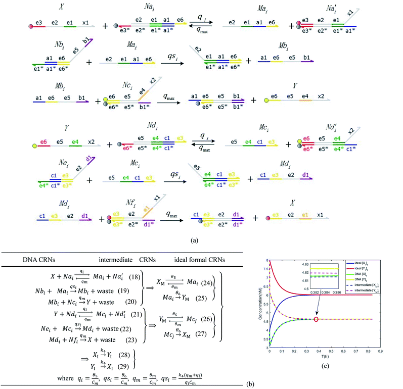 |
| | Fig. 6 Synchronization reaction module. (a) A list of DNA reactions; (b) exhibits the DNA CRNs and appropriate ideal formal CRNs, where intermediate CRNs is the transition between DNAs and ideal formal CRNs; (c) represents the process of synchronization between X and Y in DNA CRNs, intermediate CRNs and ideal formal CRNs, respectively, where Cm = 104 nM, [X]0 = [XM]0 = [XI]0 = 4 nM, and [Y]0 = [YM]0 = [YI]0 = 8 nM; qsi = 10−6 nM s−1, qi = 3 × 10⁻⁴ nM s−1 and qm = 10−3 nM s−1. In (18), X react with Nai producing Mai reversely; the producer Mai reacts with Nbi to produce Mbi in (19), and Y is produced by Mbi and Nci, which is equivalent to YI being produced by XI in ideal CRNs (28). DSD implementation of ideal reaction (29) is similar to (28). | |
I. In DNA CRNs
| | |
[X]0 + [Y]0 = [X]t + [Y]t + [Mai]t + [Mbi]t + [Mci]t + [Mdi]t
| (30) |
When DNA CRNs approach reaction equilibrium, the following can be obtained:
| |
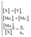 | (31) |
Considering (30) and (31), we can obtain the synchronous value:
| |
 | (33) |
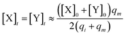
II. In intermediate CRNs
| | |
[XM]0 + [YM]0 = [XM]t + [YM]t + [Mai]t + [Mci]t
| (34) |
When intermediate CRNs approach reaction equilibrium, we can obtain
| |
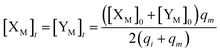 | (35) |
III. In ideal CRNs
| | |
[XI]0 + [YI]0 = [XI]t + [YI]t
| (36) |
Eqn (36) is satisfied when X1 and Y1 approach instant equilibrium through (27) and (28)
Therefore, the synchronous value of X1 and Y1 are obtained as follows:
| |
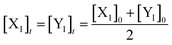 | (38) |
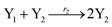
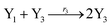
3.2. 3-Variable Lotka–Volterra oscillator
The Lotka–Volterra model is one of the earliest sound mathematical principles27–29 to describe population dynamics, and the Lotka–Volterra oscillator is known to be an ecological food chain oscillator. A 2-variable Lotka–Volterra oscillator can be described by ideal formal CRNs as follows:1| |
 | (39a) |
| |
 | (39b) |
| |
 | (39c) |
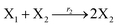
where X1 and X2 are reactants; r1, r2, and r3 represent the reaction rate of reaction (39a–c), respectively. Reaction (39a) leads to an increase in X1, and X1 can catalyze reaction (39a).
The product of X1 will increase the product X2, and X2 can catalyze reaction (39b). When the concentration of X1 increases to a certain degree, an increase in X2 will lead to consumption of X1 and the decrease in X1 will slow down reaction (39b), which can lead to a decrease in X2. Therefore, in the cycle, the concentrations of X1 and X2 will fluctuate over time.
According to the basic Lotka–Volterra oscillator, a 3-variable Lotka–Volterra oscillator model can be described by ideal CRNs as follows:
| |
 | (40a) |
| |
 | (40b) |
| |
 | (40c) |
| |
 | (40d) |
| |
 | (40e) |
CRNs (40) can be represented by the following set of ODEs:
| | |
Ẋ1 = r1X1 − r2X1X2 − r3X1X3 = F1(X1)
| (41) |
| | |
Ẋ2 = r2X1X2 − r4X2 = F2(X2)
| (42) |
| | |
Ẋ3 = r1X1X3 − r5X3 = F3(X3)
| (43) |
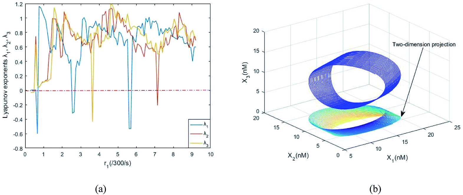
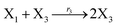
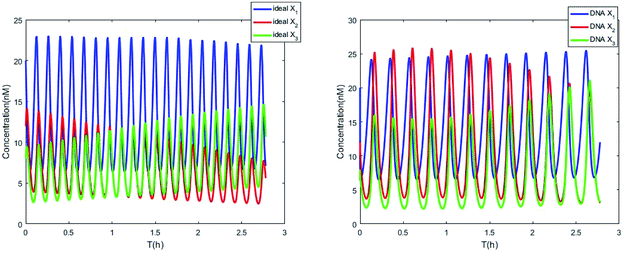
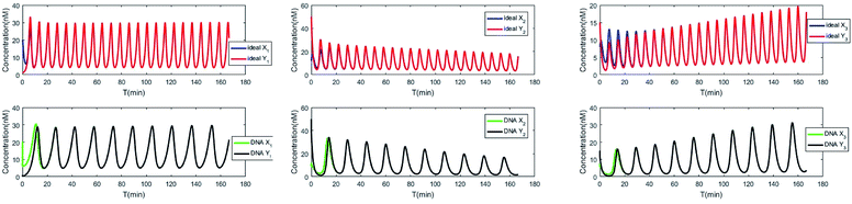
Fig. 8(a) shows the evolution of Lyapunov exponents λi (i = 1,2,3) of ideal formal CRNs (40) with the chemical reaction rate parameter, r1. It is known that the kinetic characteristics of the system can be characterized by the Lyapunov exponent, if exist in the range in which one Lyapunov exponent is positive and another Lyapunov exponent is negative, indicating that the system is at a chaotic state. Furthermore λ1 < 0, λ2 > 0 and λ3 > 0 when the parameter is taken as r1 = 5.5/300 s−1, and the phase map of the state variables X1, X2 and X3 is shown in Fig. 8(b).
 |
| | Fig. 7 Evolution of concentrations of x1, x2, x3, y1, y2 and y3 of two 3-variable Lotka–Volterra oscillator systems based on ideal CRNs and DNA intermediate CRNs, respectively. | |
 |
| | Fig. 8 (a) The evolution of Lyapunov exponents λi (i = 1, 2, 3) with the chemical reaction rate k1. (b) The chaotic attractor in the (X1, X2, X3) phase space and its two-dimension projection. | |
3.3. Synchronization of two 3-variable Lotka–Volterra oscillator systems
Considering another 3-variable Lotka–Volterra oscillator system| |
 | (44a) |
| |
 | (44b) |
| |
 | (44c) |
| |
 | (44d) |
| |
 | (44e) |
where the initial concentrations of the above two systems are different. In this study, we used four types of fluorophores as reporters: ssDNA X1 and Y1 are identified by the TYE563 fluorophore (blue ball) with λEx = 549 nm, λEm = 563 nm; ssDNA X2 and Y2 are identified by the ROX fluorophore (red ball) with λEx = 588 nm, λEm = 608 nm; ssDNA X3 and Y3 are identified by FAM fluorophore (green ball) with λEx = 495 nm and λEm = 520 nm; and the dark quencher is Lowa Black RQ.11
In order to realize internal synchronization between two chemical reaction networks, we added coupling terms as follows:
| |
 | (45a) |
| |
 | (45b) |
| |
 | (45c) |
| |
 | (45d) |
| |
 | (45e) |
| |
 | (45f) |
| |
 | (45g) |
| |
 | (45h) |
| |
 | (46a) |
| |
 | (46b) |
| |
 | (46c) |
| |
 | (46d) |
| |
 | (46e) |
| |
 | (46f) |
| |
 | (46g) |
| |
 | (46h) |
ODEs of CRNs (45) and (46) can be described as follows:
| | |
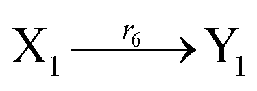
Ẋ1 = r1X1 − r2X1X2 − r3X1X3 + r6(Y1 − X1) = F1(X1) + r6(Y1 − X1)
| (47) |
| | |
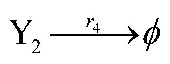
Ẋ2 = r2X1X2 + r6Y2 − r4X2 −r6X2 = F2(X2) + r6(Y2 − X2)
| (48) |
| | |
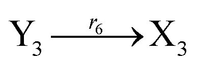
Ẋ3 = r3X1X3 + r6Y3 − r5X3 − r6X3 = F3(X3) + r6(Y3 − X3)
| (49) |
| | |
Ẏ1 = r1Y1 − r2Y1Y2 − r3Y1Y3 + r6(X1 − Y1) = G1(Y1) + r6(X1 − Y1)
| (50) |
| | |
Ẏ2 = r2Y1Y2 + r6X2 − r4Y2 − r6Y2 = G2(Y2) + r6(X2 − Y2)
| (51) |
| | |
Ẏ3 = r3Y1Y3 + r6X3 − r5Y3 − r6Y3 = G3(Y3) + r6(X3 − Y3)
| (52) |
The error state was defined as ei = yi − xi (i = 1, 2, 3), and the dynamics of error can be described as follows:
| |
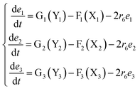 | (53) |
In simulations, the two 3-variable Lotka–Volterra oscillator systems with different initial values, and the evolution of the maximum Lyapunov exponent of eqn (53) with the chemical reaction rate r6 is given in Fig. 9. When the maximal Lyapunov exponent λm is negative, the synchronization of the two 3-variable Lotka–Volterra oscillator systems can be obtained.30
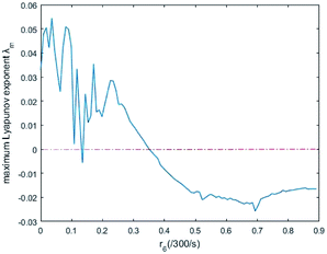 |
| | Fig. 9 The evolution of maximum Lyapunov exponent with chemical reaction rate r6. | |
CRNs (45) and (46) can be described by the abovementioned DNA reaction modules as follows:
| |
 | (54a) |
| |
 | (54b) |
| |
 | (54c) |
| |
 | (54d) |
| |
 | (55a) |
| |
 | (55b) |
| |
 | (55c) |
| |
 | (55d) |
| |
 | (55e) |
| |
 | (56a) |
| |
 | (56b) |
| |
 | (56c) |
| |
 | (56d) |
| |
 | (56e) |
| |
 | (57) |
| |
 | (58) |
| |
 | (59a) |
| |
 | (59b) |
| |
 | (59c) |
| |
 | (59d) |
| |
 | (60a) |
| |
 | (60b) |
| |
 | (60c) |
| |
 | (60d) |
| |
 | (60e) |
| |
 | (61a) |
| |
 | (61b) |
| |
 | (61c) |
| |
 | (61d) |
| |
 | (61e) |
| |
 | (62) |
| |
 | (63) |
| |
 | (64a) |
| |
 | (64b) |
| |
 | (64c) |
| |
 | (65a) |
| |
 | (65b) |
| |
 | (65c) |
| |
 | (66a) |
| |
 | (66b) |
| |
 | (66c) |
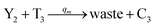
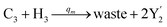
Visual DSD software can be used to realize the approximations of the CRNs (45) and (46).22 The DSD implementation of the catalysis reactions (54) and (59) are shown in Fig. 3. The DSD implementation of the catalysis reactions (55), (56), (60) and (61) are shown in Fig. 4. The reactions (57), (58), (62) and (63) are degradation reactions. The DSD implementation of reactions (57), (58), (62) and (63) are shown in Fig. 5. Reactions (64)–(66) are used as the synchronization module. The DSD implementation of reactions (64)–(66) are shown in Fig. 6.
4. Simulation results
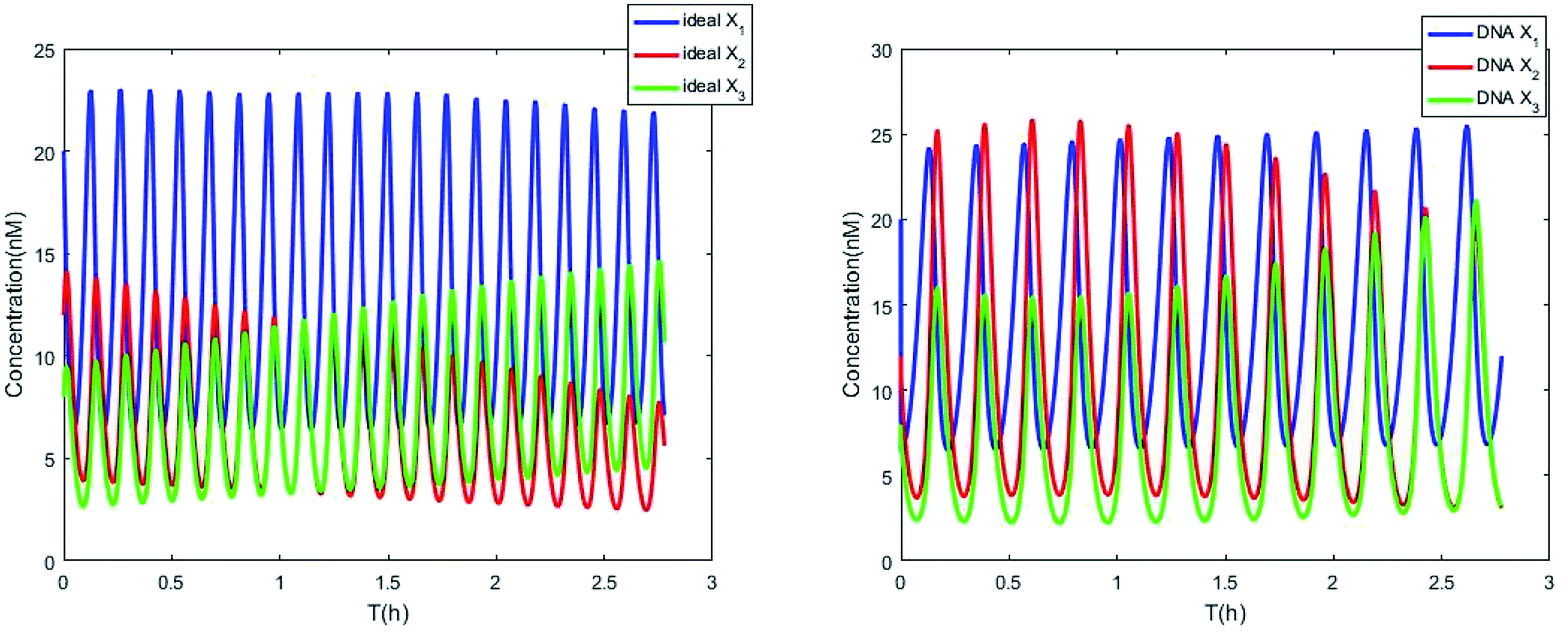
The parameters of the 3-variable Lotka–Volterra oscillator are given in Table 1, and [X1]0, [X2]0, [X3]0, [Y1]0, [Y2]0 and [Y3]0 represent the initial values of species X1, X2, X3, Y1, Y2 and Y3, respectively. [X1]0 = 20 nM, [X2]0 = 12 nM, [X3]0 = 8 nM, [Y1]0 = 1 nM, [Y2]0 = 50 nM, and [Y3]0 = 15 nM, where the values of chemical reaction rates ri, (i = 1,⋯,5) are referenced1.
Table 1 Parameter Values of the Lotka–Volterra Oscillator
| |
Values |
|
Values |
|
Values |
| r1 |
5.5/300 s−1 |
q1 |
r1C−1m |
Cm |
2 × 10⁻⁵ M |
| r2 |
106 M s−1 |
q2 |
105 M s−1 |
qm |
106 M s−1 |
| r3 |
1.008 × 10⁶ M s−1 |
q3 |
r2 |
|
|
| r4 |
4/300 s−1 |
q4 |
105 M s−1 |
|
|
| r5 |
4/300 s−1 |
q5 |
r3 |
|
|
| r6 |
0.8/300 s−1 |
q6 |
105 M s−1 |
|
|
| |
|
q7 |
r4C−1m |
|
|
| |
|
q8 |
r5C−1m |
|
|
| |
|
q9 |
2 × 10⁵ M s−1 |
|
|
| |
|
qs |
r6(qm + q9)/(q9Cm) |
|
|
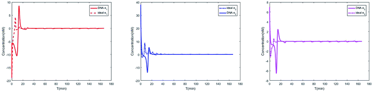
The evolution of the 3-variable Lotka–Volterra oscillator based on ideal CRNs and the 3-variable Lotka–Volterra oscillator based on DNA CRNs are shown in Fig. 7 and 8. When the three coupling terms are added to the system, the evolution of the 3-variable Lotka–Volterra oscillator based on DNA CRNs and the 3-variable Lotka–Volterra oscillator based on ideal CRNs are given in Fig. 9. According to Fig. 10, it can be found that the error between Yi and Xi (i = 1, 2, 3) approaches zero, which indicates that synchronization among Xi and Yi with different initial concentrations is realized. It is clear that errors between Xi and Yi in the ideal CRNs approach zero, which is similar to errors in DNA CRNs, as shown in Fig. 10 and 11.
 |
| | Fig. 10 Process of synchronization of two 3-variable Lotka–Volterra oscillator systems based on DNA and ideal CRNs. | |
 |
| | Fig. 11 Evolution of errors between two 3-variable Lotka–Volterra oscillator systems based on DNA and ideal CRNs. | |
In CRNs, luminous intensity relates to the concentration of DNA strands. We can observe the process of synchronization of the two 3-variable Lotka–Volterra oscillator systems through luminous intensity. The luminous intensity of Xi and Yi are different without adding coupling terms to the systems. The luminous intensity of Xi and Yi reach unanimity when there is synchronization among Xi and Yi.
5. Conclusion
We proposed a 3-variable Lotka–Volterra oscillator system as an example and realized synchronization of two 3-variable Lotka–Volterra oscillator systems with different initial concentrations. For more convenient observation and more accurate detection of synchronization, DNA strands were designed with fluorophores and quenchers. We demonstrated the contributions of fluorophores and quenchers using the CRNs modules, and analyzed the differences between DNA CRNs and ideal formal CRNs. We used Visual DSD software as a design tool for the DNA strands and CRN language to simulate the synchronization of two 3-variable Lotka–Volterra oscillator systems, one each in DNA CRNs and ideal CRNs. Numerical simulation demonstrates that the method of synchronization in this article is effective for ideal CRNs as well as DSD implementation CRNs.
Conflicts of interest
There are no conflicts to declare.
Acknowledgements
This study was supported by the National Natural Science Foundation of China (No. 61425002, 61751203, 61772100) and by the Program for Changjiang Scholars and Innovative Research Team in University (No. IRT_15R07). We thank LetPub (http://www.letpub.com) for its linguistic assistance during the preparation of this manuscript.
References
- D. Soloveichik, G. Seelig and E. Winfree, DNA as a universal substrate for chemical kinetics, Proc. Natl. Acad. Sci. U. S. A., 2010, 107, 5393–5398 CrossRef PubMed.
- R. Sawlekar, F. Montefusco, V. V. Kulkarni and D. G. Bates, Implementing nonlinear feedback controllers using DNA strand displacement reactions, IEEE Transactions on Nanobioscience, 2016, 15, 443–454 CrossRef PubMed.
- X. Olson, S. Kotani, B. Yurke, E. Graugnard and W. Hughes, Kinetics of DNA Strand Displacement Systems with Locked Nucleic Acids, J. Phys. Chem. B, 2017, 121, 2594–2602 CrossRef PubMed.
- W. Li, F. Zhang, H. Yan and Y. Liu, DNA based arithmetic function: a half adder based on DNA strand displacement, Nanoscale, 2016, 8, 3775–3784 RSC.
- J. W. Sun, X. Li, G. Z. Cui and Y. F. Wang, One-bit half adder-half subtractor logical operation based on the DNA strand displacement, J. Nanoelectron. Optoelectron., 2017, 12, 375–380 CrossRef.
- M. R. Lakin and D. Stefanovic, Supervised Learning in Adaptive DNA Strand Displacement Networks, ACS Synth. Biol., 2016, 5, 885–897 CrossRef PubMed.
- T. Song, S. Garg, R. Mokhtar, H. Bui and J. Reif, Analog Computation by DNA Strand Displacement Circuits, ACS Synth. Biol., 2016, 5, 898–912 CrossRef PubMed.
- G. Cui, J. Zhang, Y. Cui, T. Zhao and Y. Wang, DNA strand-displacement digital logic circuit with fluorescence resonance energy transfer detection, J. Comput. Theor. Nanosci., 2015, 12, 2095–2100 CrossRef.
- M. Song, Y. C. Wang, M. H. Li and Y. F. Dong, Metal-mediated logic computing model with DNA strand displacement, J. Comput. Theor. Nanosci., 2010, 12, 2318–2321 CrossRef.
- L. Qian and E. Winfree, Scaling Up Digital Circuit Computation with DNA Strand Displacement Cascades, Science, 2011, 332, 1196–1201 CrossRef PubMed.
- L. Qian, E. Winfree and J. Bruck, Neural network computation with DNA strand displacement cascades, Nature, 2011, 475, 368–372 CrossRef PubMed.
- A. J. Thubagere, C. Thachuk, J. Berleant, R. Johnson, D. Ardelean, K. M. Cherry and L. L. Qian, Compiler-aided systematic construction of large-scale DNA strand displacement circuits using unpurified components, Nat. Commun., 2017, 8 Search PubMed.
- G. Z. Cui, J. Y. Zhang, Y. H. Cui, T. T. Zhao and Y. F. Wang, DNA strand-displacement digital logic circuit with fluorescence resonance energy transfer detection, J. Comput. Theor. Nanosci., 2015, 12, 2095–2100 CrossRef.
- Z. Zhang, T. W. Fan and I. M. Hsing, Integrating DNA strand displacement circuitry to the nonlinear hybridization chain reaction, Nanoscale, 2017, 9, 2748–2754 RSC.
- M. J. Zhang, R. M. Li and L. S. Ling, Homogenous assay for protein detection based on proximity DNA hybridization and isothermal circular strand displacement amplification reaction, Anal. Bioanal. Chem., 2017, 409, 4079–4085 CrossRef PubMed.
- K. Miyakawa, T. Okano and S. Yamazaki, Cluster synchronization in a chemical oscillator network with adaptive coupling, J. Phys. Soc. Jpn, 2013, 82 CrossRef.
- A. Alofi, F. L. Ren, A. Al-Mazrooei, A. Elaiw and J. D. Cao, Power-rate synchronization of coupled genetic oscillators with unbounded time-varying delay, Cogn. Neurodyn., 2015, 9, 549–559 CrossRef PubMed.
- J. F. Totz, R. Snari, D. Yengi, M. R. Tinsley, H. Engel and K. Showalter, Phase-lag synchronization in networks of coupled chemical oscillators, Phys. Rev. E, 2015, 92 CrossRef PubMed.
- Z. Nie, P. F. Wang, C. Tian and C. D. Mao, Synchronization of two assembly processes to build responsive DNA nanostructures, Angew. Chem., Int. Ed., 2014, 53, 8402–8405 CrossRef PubMed.
- A. Apraiz, J. Mitxelena and A. Zubiaga, Studying cell cycle-regulated gene expression by two complementary cell synchronization protocols, J. Vis. Exp, 2017, 124 Search PubMed.
- D. J. Ferullo, D. L. Cooper, H. R. Moore and S. T. Lovett, Cell cycle synchronization of Escherichia coli using the stringent response, with fluorescence labeling assays for DNA content and replication, Methods, 2009, 48, 8–13 CrossRef PubMed.
- M. R. Lakin, S. Youssef, F. Polo, S. Emmott and A. Phillips, Visual DSD: A design and analysis tool for DNA strand displacement systems, Bioinformatics, 2011, 27, 3211–3213 CrossRef PubMed.
- D. Y. Zhang and E. Winfree, Control of DNA Strand displacement kinetics using toehold exchange, J. Am. Chem. Soc., 2009, 131, 17303–17314 CrossRef PubMed.
- K. Sakamoto, H. Gouzu, K. Komiya, D. Kiga, S. Yokoyama, T. Yokomori and M. Hagiya, Molecular computation by DNA hairpin formation, Science, 2000, 288, 1223–1226 CrossRef PubMed.
- J. Xie, Q. Mao, W. L. Tai Phillip, R. He, J. Z. Ai, Q. Su, Y. Zhu, H. Ma, J. Li, S. F. Gong, D. Wang, Z. Gao, M. X. Li, L. Zhong, H. Zhou and G. P. Gao, Short DNA Hairpins Compromise Recombinant Adeno-Associated Virus Genome Homogeneity, Mol. Ther., 2017 Search PubMed.
- C. B. Ma, H. S. Liu, K. F. Wu, M. J. Chen, L. Y. Zheng and J. Wang, An exonuclease I-based quencher-free fluorescent method using DNA hairpin probes for rapid detection of microRNA, Sensors, 2010, 17 Search PubMed.
- H. Matsuda, N. Ogita, A. Sasaki and K. Sato, Statistical-Mechanics Of Population – The Lattice Lotka–Volterra Model, Prog. Theor. Phys., 1992, 88, 1035–1049 CrossRef.
- Y. K. Li and Y. Kuang, Periodic solutions of periodic delay Lotka–Volterra equations and systems, J. Math. Anal. Appl., 2001, 255, 260–280 CrossRef.
- S. R. Dunbar, Traveling Wave Solutions of Diffusive Lotka–Volterra equations, Journal of Mathematical Biology, 1983, 17, 11–32 CrossRef.
- P. Badola, S. S. Tambe and B. D. Kulkarni, Driving systems with chaotic signals, Phys. Rev. A, 1992, 46, 6735–6737 CrossRef.
|
| This journal is © The Royal Society of Chemistry 2018 |
Click here to see how this site uses Cookies. View our privacy policy here. 
 Open Access Article
 This Open Access Article is licensed under a Creative Commons Attribution-Non Commercial 3.0 Unported Licence
 *ab
*ab


 hybridization at the end of the branch migration, the loop portion a2 – b1 – b2 of the hairpin is protected if it does not open.
 is produced by XM in (5), and the increase in
  will catalyze (6), while the producer XM can catalyze the production of
  . According to (1), d[X]t/dt = −qiCm[X]t and d[XM]t/dt = −θ1[XM]t by (5); if DSD (1) and (2) can approximate to the intermediate (5), qi = θ1/Cm is obtained. According to (3), d[X′]t/dt = −qmCm[X′]t, while
  based on (6). If DSD (3) and (4) can approximate to the intermediate (6), qm = θm/Cm. d[X]t/dt = −θ2[X]t and d[XM]t/dt = −qjCm [XM]t, according to (4) and (6); if (4) is equivalent to (6), qj = θ2/Cm. Similarly, we can obtain k1 = θ1 based on (5), (6) and (7). Initial concentrations of the auxiliary species
  and
and  are set to Cm, where [X]0 ≪ Cm, and [X]0, [Y]0 are the initial concentrations of X and Y. As shown in Fig. 3(c), the evolutions of X in DNA CRNs, intermediate CRNs and ideal CRNs are approximately coincident. This shows that DNA CRNs, intermediate CRNs and ideal formal CRNs in the catalysis reaction module (1) are equivalent, but there are nuances between DNA CRNs, intermediate CRNs and ideal formal CRNs.
 to displace
  in (1),
  releases two X′ in (2). In (3), species X′ reacts with hairpin
  to produce
  , and
, and  and releases X in (4) on reaction with
  . This reaction replaces the ssDNA strand without the fluorophore to the ssDNA strand with the fluorophore, as adapted from.4 qm represents a maximum strand displacement rate constant under the assumption of equal binding strength for all full toeholds; when qi and ki are satisfied qi,qj ≪ qm, ki ≪ qmCm; [X]0 and Cm are satisfied [X]0 ≪ Cm, as adapted from.1
 is produced by XM and YM in (13), and the increase in
  will catalyze (14), while the producer YM can catalyze the production of
  and consumption of XM. According to ref. 1, we have. qi = θ3. Similar to catalysis reaction module (1), qj = θ4/Cm, qm = θm/Cm and k2 = θ3. Initial concentrations of the auxiliary species Ai, Bi, Hi, Pj, Spj, and Sqj are set to Cm, where [X]0, [Y]0 ≪ Cm. As shown in Fig. 4(c), the evolutions of Y in DNA CRNs, intermediate CRNs and ideal CRNs are approximately coincident. This indicates that DNA CRNs, intermediate CRNs and ideal CRNs in catalysis reaction module (2) are equivalent, but there are nuances between DNA CRNs, intermediate CRNs and ideal CRNs.
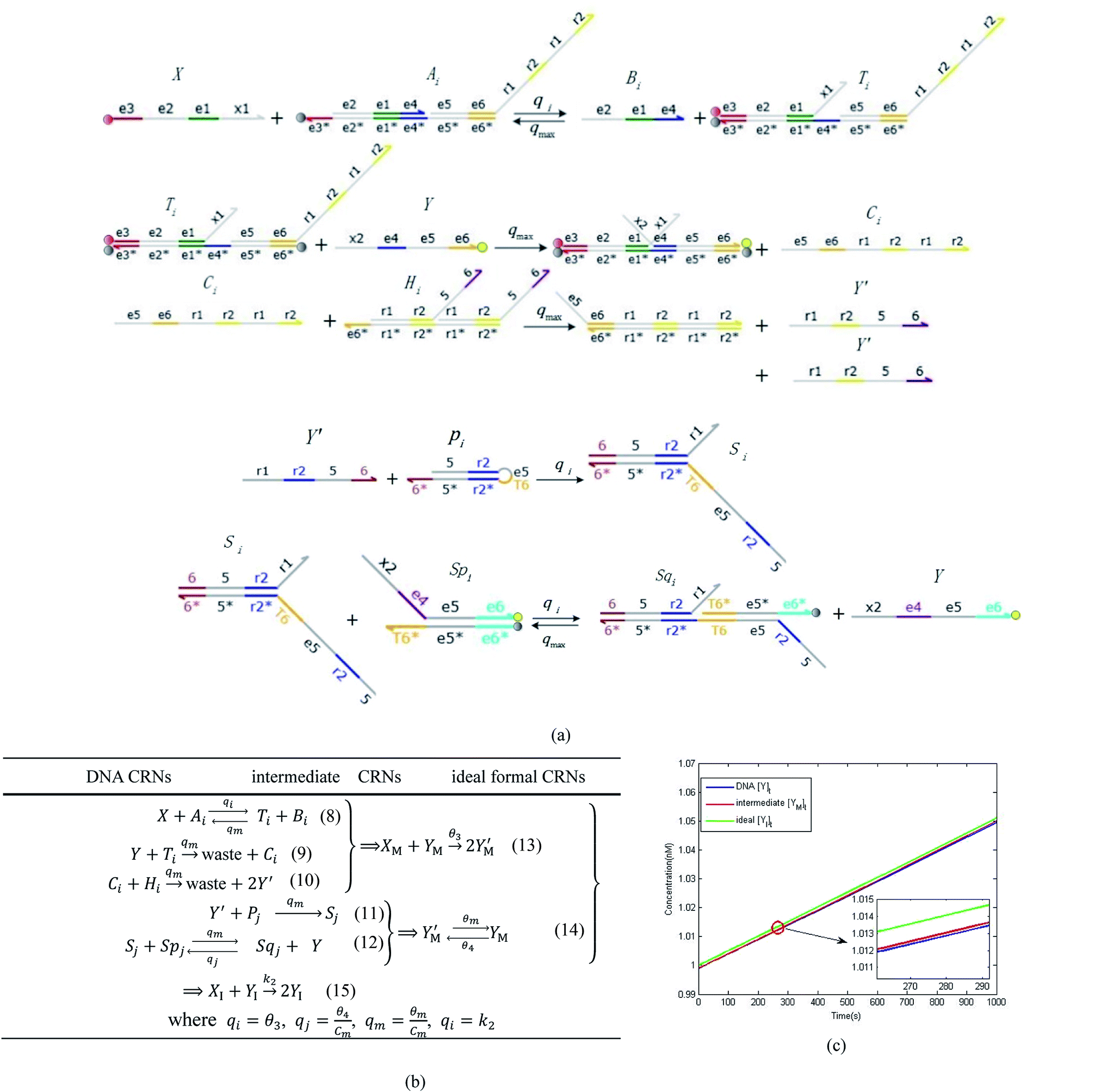
 is gained by species XM and YM in intermediate CRN (13). Species X reacts with Ai to displace Ti. In (9), Ci is produced when Y irreversibly displaces Ti, and Hi releases 2 Y′ in reaction (10), as adapted from.1 In (11), species Y′ reacts with hairpin Pj to produce Sj, and Sj releases X in (12) on reacting with Spj, as adapted from.4
 , Nbi, Nci, Ndi,
  , Nei, and Nfi are set to Cm, where [X]0,[Y]0 ≪ Cm. Fig. 6(c) shows that X and Y can share the same dynamic behavior in DNA CRNs, intermediate CRNs and ideal formal CRNs, but their synchronous values are different. The reasons for this phenomenon are as follows: