Clustering and dynamics of particles in dispersions with competing interactions: theory and simulation

Abstract

Dispersions of particles with short-range attractive and long-range repulsive interactions exhibit rich equilibrium microstructures and a complex phase behavior. We present theoretical and simulation results for structural and, in particular, short-time diffusion properties of a colloidal model system with such interactions, both in the dispersed-fluid and equilibrium-cluster phase regions. The particle interactions are described by a generalized Lennard-Jones-Yukawa pair potential. For the theoretical-analytical description, we apply the hybrid Beenakker–Mazur pairwise additivity (BM-PA) scheme. The static structure factor input to this scheme is calculated self-consistently using the Zerah-Hansen integral equation theory approach. In the simulations, a hybrid simulation method is adopted, combing molecular dynamics simulations of colloids with the multiparticle collision dynamics approach for the fluid, which fully captures hydrodynamic interactions. The comparison of our theoretical and simulation results confirms the high accuracy of the BM-PA scheme for dispersed-fluid phase systems. For particle attraction strengths exceeding a critical value, our simulations yield an equilibrium cluster phase. Calculations of the mean lifetime of the appearing clusters and the comparison with the analytical prediction of the dissociation time of an isolated particle pair reveal quantitative differences pointing to the importance of many-particle hydrodynamic interactions for the cluster dynamics. The cluster lifetime in the equilibrium-cluster phase increases far stronger with increasing attraction strength than that in the dispersed-fluid phase. Moreover, significant changes in the cluster shapes are observed in the course of time. Hence, an equilibrium-cluster dispersion cannot be treated dynamically as a system of permanent rigid bodies.

---

1 Introduction

Brownian particle dispersions exhibiting short-range attractive (SA) and long-range repulsive (LR) interactions, such as low-salinity lysozyme protein solutions and suspensions of micron-sized charged colloidal particles with added small depletants, have been intensely studied over the past years.^1–10 Such systems, referred to as SALR dispersions, exhibit a rich phase behavior, including equilibrium fluid and cluster phases, and nonequilibrium phases such as random and cluster-percolated phases.^{2,3,5–7,11–13} These investigations were triggered by the experimental observation of a low-wavenumber, q, (low-q) peak in the static structure factor S(q), indicative of intermediate-range microstructural ordering (IRO), arising from the competing SA and LR interactions.^1,4 The competition of SA- and LR-potential contributions can lead to the occurrence of IRO, and the formation of equilibrium clusters. The existence of such clusters necessitates a delicate balance between SA, favoring aggregation, and LR suppressing macroscopic phase separation. SALR-type protein systems are particularly interesting, since the clustering of proteins can result in severe diseases such as Alzheimer and Parkinson,^14,15 and cateract formation.¹⁶

In contrast to the multitude of studies on static properties of SALR systems,^9,17 comparably little is known about their dynamical aspects. A major challenge for simulation and theoretical studies of the dynamics of these systems is to account for solvent-mediated hydrodynamic particle interactions (HIs) which decisively influence diffusion and rheology. HIs are long-ranged, and, in general, non-pairwise additive for larger particle concentrations. In earlier studies,² Brownian dynamics simulations based on the generalized Lennard-Jones–Yukawa SALR model potential have been performed, where the salient HIs were completely disregarded. In these simulation studies, the dynamic structure factor, S(q,t), as a function of correlation time t and wavenumber q, and the wavenumber-dependent short-time diffusion function, D(q), have been determined.

The theoretical description of cluster-phase states is further hampered by the occurrence of additional time and length scales associated with the distributions of particle-cluster lifetimes, cluster sizes and shapes, and cluster electric charges. This renders a clear distinction between colloidal short-time and long-time regimes complicated, in contrast to homogeneous suspensions of individually diffusing monodisperse particles. An interesting experimental finding exemplifying the intriguing dynamics of SALR systems was obtained by Liu et al. in ref. 4. The short- and long-time self-diffusion coefficients for salt-free lysozyme protein solutions, deduced from neutron spin echo (NSE) measurements, were found to exhibit roughly the same concentration dependence. Lysozyme solutions, however, are special SALR systems due to the non-isotropic short-range patchy attractions between the lysozyme proteins.^18,19 In this context, by using mesoscale hydrodynamics simulations, the strong influence of particle surface patchiness on short-time diffusion properties was shown recently.²⁰ The patchy SA-interaction contribution gives rise to smaller values of the cage diffusion coefficient D(q_m), where q_m is the location of the particles next neighbor peak in S(q), than those observed for isotropic attraction of comparable strength and range.

A comprehensive theoretical study of short-time dynamic properties of SALR systems in the dispersed-fluid phase has been presented,^18,21 where the analytic hybrid Beenakker–Mazur (plank) pairwise-additivity (BM-PA) scheme for calculating D(q) has been used. This scheme requires the static structure factor, or likewise the associated radial distribution function, as the only input. The BM-PA method gives overall good results for the short-time diffusion properties, both of neutral and charge-stabilized particle dispersions, which was shown in comparison with elaborate hydrodynamic force-multipole simulations and experimental data on various colloidal systems.^22–24 Interestingly, a non-monotonic dependence of the sedimentation velocity of SALR dispersions on the interaction strength parameter is predicted by this method,²¹ revealing the intricate influence of short-range attractive and long-range repulsive pair potential contributions on the short-time dynamics.

In the present paper, we study the short-time dynamics of SALR systems both in the monomer-dominated dispersed-fluid and the equilibrium-cluster phases. We assess the particle dynamics by employing both a mesoscale hydrodynamic simulation method, the multiparticle collision dynamics (MPC) approach, and the aforementioned analytic BM-PA scheme. MPC is a particle-based simulation technique which incorporates thermal fluctuations, provides hydrodynamic correlations,²⁵ and is easily coupled with other simulation techniques such as molecular dynamics simulations for embedded particles.^26–28 It has been successfully applied to study equilibrium and non-equilibrium dynamical properties of colloids,^29–39 polymers,^40–47 blood cells,^48,49 and biological microswimmers.^50–52 Specifically, MPC simulations account for the many-particle HIs in the overdamped Brownian dynamics regime of friction-dominated particle motion addressed in the present work.

From the comparison with our MPC simulation results, we demonstrate the high accuracy of the hybrid BM-PA scheme for systems in the dispersed-fluid phase. In addition, we explore the inter- and intra-cluster dynamics in the equilibrium-cluster phase by simulations, and determine the characteristic cluster lifetime also in comparison with analytic first-passage time calculations. The intra-cluster dynamics in the equilibrium-cluster phase of SALR systems is of special interest, and here in particular the influence of the HIs. If the particles forming a cluster can move individually, i.e., if the cluster is non-rigid, there is no hydrodynamic screening inside the cluster. In fact, it is well known that HIs between an ensemble of interacting mobile particles is not screened owing to momentum conservation,^53,54 and this is shown quantitatively in a recent Stokesian dynamics simulation study.⁵⁵ The absence of HIs screening in turn implies that a polydispersity model describing the SALR dispersion as a mixture of differently sized rigid clusters is not appropriate, at least regarding the system dynamics. Our simulations clearly reveal internally very dynamic clusters, and a cluster lifetime which depends significantly on HIs. This emphasizes the importance of HIs in the dynamics of the particles also in the equilibrium-cluster phase.

The paper is structured as follows. Section 2 comprises the presentation of the modified-LJY model system of spherical Brownian particles under SALR conditions, a short description of the analytic BM-PA approach, and of the MPC simulation method. Section 3 presents results for structural properties and the phase behavior. Dynamical aspects are discussed in Section 4. Summary and conclusions are given in Section 5.

2 Theoretical description

2.1 Dispersion interaction potential

The effective interaction between dispersed particles with SALR-type forces is frequently modeled by the hard-core two-Yukawa or the modified Lennard-Jones–Yukawa (LJY) pair potentials (see, e.g., ref. 3, 5, 21 and 56). Since the hard-core part of the two-Yukawa potential renders dynamical simulations rather demanding, we use a steep Lennard-Jones-type (LJ) potential for the short-range repulsive interaction. Simultaneously, we capture the short-range attractive interaction by this potential. The long-range repulsion is accounted for by a repulsive Yukawa potential. Hence, the LJY pair potential readswhere x = r/σ, with r the particle center-to-center distance and σ = 2a the particle diameter, and β = 1/k_BT, with T the temperature and k_B Boltzmann's constant. Here, ε is the strength of short-range attraction/repulsion, and A characterizes the strength of the long-range repulsion. The parameter A is related to the square of the effective electric charge of a colloidal particle,^6,57 and ξ is accordingly the electrostatic Debye screening length in units of σ. We emphasize that the occurrence of a low-wavenumber IRO peak in the static structure factor at a wavenumber smaller than that corresponding to the particles next-neighbor peak is a common feature of SALR systems, and not specific to a particular pair potential.

The phase behavior of the LJY model system for fixed potential parameter values A = 2, ξ = 1.794, and varying values of ε has been studied by MD simulations and the thermodynamic Gibbs–Duhem integration method.⁶ Thereby, the selected reduced screening length ξ corresponds, for a typical particle diameter of σ ≈ 100 nm, to a 1 : 1 aqueous electrolyte solution at a concentration of about 3 μM.⁶ The shape of the LJY potential for these parameters, and various attraction strengths ε, is shown in Fig. 1. The minimum of the potential is located at x_min = 1.014, where βV(x_min) ≈ 2 − ε (cf.Fig. 1). The range of attraction strengths considered in this work is ε = 0–8. The second zero-crossing x₀ > x_min of V(x) is x₀ ≈ 1.032 for ε = 3 and x₀ ≈ 1.06 for ε = 8. Here, x₀ characterizes the radial position of the comparably small interval x_min < x < x_max of short-range attraction, where V′(x) = 0 at x_max in the interval x_min < x < ξ.

Fig. 1 The generalized Lennard-Jones–Yukawa (LJY) potential of eqn (1) for various values of the reduced attraction strength ε, as indicated, and the fixed values A = 2 and ξ = 1.794 for the strength and range of the long-range Yukawa-repulsion part, respectively.

2.2 Theoretical approach

2.2.1 Zerah–Hansen integral equation scheme. For calculating the radial distribution function g(r) and the associated static structure factor S(q) of the LJY model system of spherical particles, we use the thermodynamically self-consistent Zerah–Hansen (ZH) integral equation scheme.⁵⁸ This method is well suited for pair potentials with a soft attractive part. Its high accuracy for hard-core two-Yukawa systems in the dispersed-fluid phase state has been recently established by a comparison with Monte Carlo simulation results for g(r).^10,21 For simplicity, we take the attraction strength ε in eqn (1) and the self-consistently determined mixing parameter in the ZH closure relation as concentration-independent, when performing the concentration derivative of the virial pressure to enforce thermodynamic self-consistency. We note here that alternative self-consistent integral equation schemes, such as the modified HNC scheme by Rosenfeld and Ashcroft⁵⁹ and the self-consistent Bomont–Bretonnet^60,61 scheme, were shown to be of comparable accuracy. The importance of imposing thermodynamic self-consistency for the employed integral equation scheme has been emphasized in ref. 62.

2.2.2 Short-time diffusion of Brownian particles. Regarding the Brownian dynamics of colloidal particles, the short-time regime τ_B ≪ t ≪ τ_D is distinguished from the long-time regime t ≫ τ_D. Here, t denotes the time, τ_B is the characteristic relaxation time of particle velocity fluctuations, and τ_D = σ²/(4d₀) is a characteristic diffusion time, where σ is the Brownian particle diameter and d₀ = k_BT/(3πη₀σ) is the single-particle translational diffusion coefficient in the solvent of viscosity η₀. For t ≪ τ_D, changes in the particles structural configurations are so minuscule that the direct influence of the pair interactions in eqn (1) on diffusional properties is not yet operative. This is different for the solvent-mediated HIs which act quasi-instantaneously even on the colloidal short-time scale. Short-time transport properties, such as the short-time self-diffusion coefficient, are thus expressible as genuine equilibrium averages, where direct interactions are only indirectly influential through their effect on the equilibrium microstructure encoded, e.g., in g(r) and S(q). Long-time dynamic transport properties such as the long-time self-diffusion coefficient and the steady-shear suspension viscosity, are influenced, additionally to HIs, by the non-hydrodynamic direct interactions in form of non-instantaneous caging (memory) effects.

The short-time dynamics of Brownian particles can be probed experimentally by measuring the q-dependent dynamic structure factor, S(q,t), using dynamic light scattering (DLS) or neutron spin echo spectroscopy (NSE), depending on the particle size, concentration, and other system properties. For short times, S(q,t) decays single exponentially, and it can be expressed in terms of the short-time diffusion coefficient D(q) as

S(q,t ≪ τ_D) = S(q)exp(−q²D(q)t). (2)

Here,characterizes the decay of concentration fluctuations of wavelength 2π/q. It is proportional to the ratio of the so-called hydrodynamic function, H(q), and the static structure factor. The former is a dynamic quantity characterizing the effect of HIs on short-time self- and collective diffusion. It can be expressed as an equilibrium average including the hydrodynamic mobility matrix, μ_ij, for an instant many-particle configuration, relating the hydrodynamic force on particle j to the velocity change of particle i caused by the solvent-mediated HIs.⁶³ In the hypothetical case of hydrodynamically non-interacting particles, where , with the unit tensor , it follows that H(q) = 1 independent of q and the particle volume fraction ϕ. Note that H(q) can be split into self and distinct parts,where the wavenumber-independent first part, invoking the average over the diagonal mobility matrix element μ_ii, is equal to the translational short-time self-diffusion coefficient d_s divided by d₀. Due to the increasing importance of the near-distance part of the HIs with increasing concentration, d_s decreases and becomes smaller than d₀. The wavenumber-dependent second part, H^d(q), is a consequence of hydrodynamic cross correlations for which i ≠ j, and it vanishes for q → ∞.

2.2.3 BM-PA hybrid scheme of short-time diffusion. Our BM-PA hybrid scheme for the calculation of H(q) consists of the second-order Beenakker–Mazur (BM) mean-field method^53,64,65 for the calculation of H^d(q), and the pairwise additivity (PA) approximation for d_s.^23,66 This scheme combines the advantages of the BM and PA methods. The PA approximation fully accounts for two-body hydrodynamic interactions including lubrication effects. Lubrication is important in particular for self-diffusion, since μ_ii decays quickly with increasing particle pair distance r as [scr O, script letter O] (1/r⁴). In contrast, the BM method is well suited for the calculation of H^d(q). Different from the PA method, it includes three-body and higher-order HIs contributions in an approximate way, thus accounting for the shielding of HIs between a particle pair by intervening particles. The BM method disregards lubrication which, however, is less significant for H^d(q). For more details about the BM-PA hybrid scheme and its earlier applications to colloidal dispersions of spherical particles including hard spheres, charge-stabilized particles, proteins, and hydrodynamically structured particles such as microgels, we refer to ref. 10, 22, 23, 66, and 67.

We assess here, by the comparison with elaborate MPC simulations, the applicability of the BM-PA method to SALR systems for the first time quantitatively. Notice that it is not clear a priori whether the BM-PA method applies to SALR systems, where intermediate-range ordering is accompanied by a larger likelihood of near-contact configurations than for purely repulsive particle systems.

2.3 Simulation method

2.3.1 Dispersion model. In the simulations, we model a spherical dispersion particle by a set of N_s = 60 point particles of mass M homogeneously distributed over the surface of a sphere of diameter σ, and an additional point particle at the center of the sphere.³⁷ In order to maintain the spherical shape, the point particles are connected with their nearest neighbors and the center particle via a harmonic potential of the formwhere R is the distance between a pair of points, and R₀ is the preferred bond length. In addition, any two dispersion particles interact with each other through the LJY potential of eqn (1) between their centers.

The dynamics of a point particle is described by Newton's equation of motion, which is solved via the velocity Verlet algorithm with the forces derived from the above potentials.⁶⁸

The simulations of ref. 37 demonstrate that this model closely resembles a hard-sphere colloidal particle with no-slip boundary conditions in a dilute dispersion. In particular, the flow field determined for an individually sedimenting MPC-colloidal sphere agrees very well with the theoretical expression for an isolated colloidal hard sphere. However, due to discretization, the hydrodynamic radius is somewhat larger than the radius a. The actual value depends on the radius of the colloid and the size of the simulation box. Explicit values are provided in Section 2.3.4.

2.3.2 Multiparticle collision dynamics fluid. The embedding MPC fluid is described by N point particles of mass m with positions r_i and velocities v_i (i = 1,…,N). Their dynamics proceeds through discrete streaming and collision steps. During streaming, the particles move ballistically and their positions are updated as

r_i(t + h) = r_i(t) + hv_i(t), (6)

where the time step h is denoted as collision time. In the collision step, the periodic simulation box is partitioned into cubic collision cells of length ã to define the interaction environment, and the particles are sorted into these cells. Particles in a collision cell interact with each other through a momentum-conserving stochastic process. We apply the Stochastic Rotation Dynamics (MPC-SRD) version of MPC,^27,28,69 where the relative velocity of each particle, with respect to the center-of-mass velocity of the cell, is rotated by a fixed angle α around a randomly oriented axis, i.e.,

v_i(t + h) = v_cm(t) + R(α)(v_i(t) − v_cm(t)). (7)

Here, v_cm is the center-of-mass velocitywith N_c the number of MPC particles in the respective collision cell, and R(α) the rotation matrix. The orientation of the rotation axis is chosen independently for every collisions cell and collision step. Moreover, the collision cells are shifted randomly before each collision step to ensure Galilean invariance.⁶⁹

2.3.3 Coupling of dispersion particle and MPC fluid. The coupling between the MPC fluid and a dispersion particle is achieved by inclusion of the point particles comprising the dispersion particle in the MPC collision step, i.e., the point particle velocities are updated according to eqn (7), which ensures momentum exchange between the particle and fluid and thereby an effective no-slip boundary condtion. The center-of-mass velocity of a collision cell containing N^c_c dispersion point particles is given bywhere V_k(t) is the velocity of a point particle k.

To maintain the temperature of the system at a desired value, we use a collision-cell level thermostat, referred to as Maxwell–Boltzmann scaling (MBS) method.⁷⁰ This ensures that a canonical ensemble is simulated.^70,71

2.3.4 Simulation parameters. The dispersion particle diameter is chosen as σ = 2a = 6ã, and the mass of a constituting point as M = 10 m to ensure correct hydrodynamic behavior.³⁷ Moreover, we apply the collision angle α = 130°, the collision time h = 0.1t₀, where is the MPC time unit, and the mean number 〈N_c〉 = 10 of MPC particles per collision cell. This yields the viscosity .⁷¹ The time step for the integration of Newton's equations of motion is set to h/10. A spring constant of K = 3000k_BT/ã² is chosen to maintain the spherical shape of a dispersion particle. Periodic boundary conditions are applied, with the lengths of the cubic simulation box of L/ã = 150 and 100 for the densities ρ* = ρσ³ = 0.1 and 0.2, respectively. This choice of parameters yields a hydrodynamic radius, which deviates from the radius σ/2 by less than 10% as determined by the translational diffusion coefficient and the flow field of a sedimenting colloid.³⁷

In the following, we will compare simulation results with analytical calculations in the overdamped time regime. This requires that the characteristic time scale for Brownian motion τ_B = N_sM/γ_s, momentum diffusion (hydrodynamics) τ_ν = a²/ν, and diffusion of a dispersion particle across its own radius τ_D = γ_sa²/k_BT obey the relation τ_B ≲ τ_ν ≪ τ_D,³¹ where γ_s = 6πη₀a is the Stokes friction coefficient of a sphere, and ν = η₀ã³/m〈N_c〉 is the kinematic viscosity. With the above parameters, these relations are satisfied, specifically τ_ν/τ_D < 5 × 10⁻³. In the subsequent chapters, we will consider time scales t/τ_ν > 1 only.

3 Phase behavior and microstructure

Fig. 2(a) displays the static structure factors, S(q), obtained by the ZH calculations and MPC simulations of LJY systems in the dispersed-fluid phase for ρ* = ρσ³ = 0.1, where ρ is the dispersion-particles density, and the attraction strengths ε = 2, 4, and 6. Consistent with previous results for SALR systems with a two-Yukawa pair potential,^21,62 our self-consistent ZH results for S(q) are also in excellent agreement with the MPC simulation results. With increasing ε, and correspondingly increasing depth of the potential well, a pronounced IRO peak of S(q) is found at a wavenumber q_c distinctly smaller than that corresponding to the particles next-neighbor distance. This peak shifts to smaller q values with increasing ε. In addition, Fig. 2(b) depicts MPC simulation results for ε = 7 and 8. For these large attraction strengths, the ZH scheme does not converge any more. The IRO peak heights following from simulations for these ε values clearly exceed the critical value of S_crit(q_c) ≈ 2.7, an empirical criterion signaling a first-order phase transition from the dispersed-fluid to the equilibrium-cluster phase,⁵ a transition observed in SALR systems at lower volume fractions. The width of the IRO peak of S(q) provides another criterion for localizing the transition from the dispersed-fluid to the equilibrium-cluster phase, owing to its relation to an IRO thermal correlation length obtained from a quadratic Ornstein–Zernike fit of S(q_c)/S(q).⁷² The location of the phase transition is most robustly predicted by the combination of both criteria for the height and width of the IRO peak.¹⁷

Fig. 2 Static structure factor, S(q), of LJY systems at reduced particle concentration ρ* = ρσ³ = 0.1, for the indicated interaction strengths ε. Simulation results are displayed by symbols and theoretical ZH integral equation predictions by solid lines. (a) MPC simulation and theoretical results of the dispersed-fluid phase for ε = {2, 4, 6}. (b) MPC simulation results for dispersed-fluid phase systems with ε = {2, 4, 6} (open symbols), and equilibrium-cluster phase systems with ε = {7, 8} (filled symbols). The horizontal dashed line in (b) marks the critical value S_crit(q_c) ≈ 2.7 for a first-order transition according to Godfrin et al. in ref. 5.

Typical microstructural snapshots from simulations are displayed in Fig. 3. We identify here two phases, namely a dispersed-fluid phase at small attraction strengths and an equilibrium-cluster phase at larger ε. The emerging clusters in the latter case are clearly visible.

Fig. 3 Simulation snapshots of the microstructure of a LJY system at concentration ρ* = 0.1. (a) A dispersed-fluid phase structure is obtained for ε = 2, and (b) an equilibrium-cluster phase structure for ε = 7. The various colors indicate dispersion particles belonging to clusters of different sizes (see left vertical color bar).

Insight into the phase behavior of the LJY system is gained from the cluster-size distribution function (CSD) defined as

where N(s) is the average fraction of particles that are members of a cluster of size s.³ Here, 〈⋯〉 is the average over representative particle configurations, n(s) is the number of clusters of size s within a given configuration, and N_p denotes the total number of dispersion particles in the simulation box, hence, . A cluster is defined by applying a distance criterion according to which the center-to-center distance |r_ij| between two particles i and j of same the cluster obeys the condition |r_ij| < r_cluster, with the cut-off distance r_cluster. We use r_cluster = x_maxσ, where x_max > 1 is the location of the maximum of V(x) (cf.Fig. 1). We confirm that a small change in the definition of the cutoff-distance, e.g., to r_cluster = x₀σ does not significantly change the shape of the CSD. Here, x₀ is the second zero-crossing of V(x) for x > 1. From the shape of N(s), so far, four different phases have been identified in SALR systems constituting a generalized phase diagram, namely the dispersed-fluid, random-percolated, equilibrium-cluster, and percolated-cluster phases.⁵

We focus here on the microstructure and dynamics of the dispersed-fluid and equilibrium-cluster phases. In the dispersed-fluid phase, N(s) is monotonically decaying with increasing s, as shown in Fig. 4, which indicates a monomer-dominated dispersion, where only transient small clusters are formed, corresponding to a mean cluster size of N̄ = 1–3. In contrast, the distribution function in the equilibrium-cluster phase exhibits a second maximum (peak) at a particular cluster size s* > 2, in addition to the monomer peak at s = 1. The second local peak reflects equilibrium clusters with a preferred size around s*, coexisting in thermodynamic equilibrium with the monomers.

Fig. 4 Distribution of cluster sizes, N(s), obtained from simulation configurations as function of the cluster size s, for A = 2, ξ = 1.794, and the indicated attraction strengths ε. The concentration is ρ* = 0.1 and in the inset ρ* = 0.2. For dispersed-fluid phase systems, open symbols connected by dashed lines are used, while equilibrium-cluster phase systems are marked by filled symbols connected by solid lines. Additionally, the inset shows a typical equilibrium cluster for ε = 7 and ρ* = 0.1. Two dispersion particles are part of a cluster for distances r ≤ r_cluster = x_maxσ, where x_max > 1 is the location of the first maximum of V(x) (cf.Fig. 1).

From the shape of the CSD functions at ρ* = 0.1, the systems with ε = 2 and 4 are identified as belonging to the dispersed-fluid phase, while the systems with ε = 7 and 8 are part of the equilibrium-cluster phase. This classification is in accord with the ε–ρ* LJY-phase diagram of ref. 6 obtained for the same potential parameters (A = 2 and ξ = 1.794) (cf.Fig. 5), as well as the phase transition criterion S(q_c) ≳ 2.7 of ref. 5. Note that for ε = 6, a shallow peak at s* > 1 appears, but the monomer peak at s = 1 still dominates. A close inspection of the simulation configurations suggests that the system for ε = 6 is still in the dispersed-fluid phase. This conclusion is supported by the schematic phase diagram of ref. 6 (see also Fig. 5, where the system with ρ* = 0.1 and ε = 6 is inside the dispersed-fluid phase region.)

Fig. 5 Schematic ε–ρ* phase diagram deduced from our MPC-generated cluster size distribution functions for the eight considered LJY systems. Open circles and filled circles label systems in the dispersed-fluid and equilibrium-cluster phases, respectively, according to the CSD shapes. The two uniformly colored areas mark the dispersed-fluid (red) and equilibrium-cluster (blue) phase regions of the LJY system as predicted in our simulation studies (see also ref. 6).

Pair correlation functions, g(r), obtained from ZH calculations and simulations are compared in Fig. 6 for ρ* = 0.1. For the dispersed-fluid phase systems, excellent agreement between analytical and simulation results is observed (cf.Fig. 6(a)). Note that the simulation results show two additional small peaks at x ≈ 1.67 and 1.75 for ε = 6. This again reflects that this system is close to the boundary separating the dispersed-fluid form the equilibrium-cluster phase. The g(r)'s of the systems in the equilibrium-cluster phase exhibit sharp peaks at various distinct positions indicating strong local ordering (Fig. 6(b)). The positions of the peaks can be attributed to preferred geometric particle configurations such as an in-line configuration of three particles (peak at x ≈ 2), an octahedral arrangement of four particles (peak at x ≈ 1.66), formation of two equilateral triangles with a common side (peak at x ≈ 1.76),¹³ and a cubic arrangement (peak at x ≈ 1.43).

Fig. 6 Radial distribution functions, g(r), for the dispersions of Fig. 2 with ρ* = 0.1 and indicated ε values. (a) MPC (symbols) and ZH (solid lines) results for three systems in the dispersed-fluid phase. (b) MPC results for two systems in the equilibrium-cluster phase. The depicted cluster configurations and the arrows indicate the cluster structures associated with the respective peaks in g(r).

Similarly, good agreement between ZH and MPC results for g(r) and S(q) is observed for the dispersed-fluid phase systems at the larger concentration ρ* = 0.2 and for ε ≤ 5, as displayed in Fig. 7. The system with ε = 6 belongs to the equilibrium-cluster phase. This follows from the respective N(s) shown in the inset of Fig. 4, and is in accord with the phase diagram of Mani et al. in ref. 6. The ZH results for S(q) and g(r) at ε = 6 significantly differ from the simulation data, in particular around the IRO peak position at q_c ≲ 2.5. Interestingly, g(r) for the equilibrium-cluster phase system with ε = 6 has a broad peak at larger x that starts roughly at x_c = 2π/q_c and becomes more pronounced with increasing S(q_c) (see inset of Fig. 7(b)). However, as it was shown recently,¹⁰ such a broad peak in g(r), visible here in the range 3 < x_c < 5, does not necessarily imply an IRO peak in the corresponding S(q).

Fig. 7 MPC simulation (symbols) and ZH (solid lines) results for (a) S(q) and (b) g(r) at ρ* = 0.2 for the indicated ε values. Filled symbols: Simulation results for the equilibrium-cluster phase system (ε = 6). Open symbols: dispersed-fluid phase systems (ε = 4 and 5). In (b), the blue line is a guide to the eye of the MPC distribution function. The inset shows g(r) for pair distances r = xσ related to the IRO structure factor peak position q_cσ for which x_c = 2π/q_cσ.

A relation was recently established between the IRO wavenumber q_c, or likewise the average center-to-center distance of clusters estimated by 2π/q_c, the mean particle number of clusters, and the dispersion particles concentration ρ*, which reads¹⁷

Table 1 lists values of the two (reduced) lengths on the left and right-hand side of eqn (11), for the considered LJY systems. Evidently, there is very good agreement between the two lengths for ρ* = 0.1, consistent with the conclusion in ref. 17. However, for the larger concentration ρ* = 0.2, there are differences of about 20–30%.

Table 1 Characteristic lengths defined by the left- and right-hand sides of eqn (11), respectively, for concentrations ρ* and interaction strengths ε as listed

ρ*	ε	2π/(qcσ)	(N̄/ρ*)^1/3
0.1	6	3.57	3.34
	7	4.17	4.11
	8	4.17	4.31
0.2	5	2.78	3.35
	6	3.33	4.17

---

Following ref. 72, we have also analyzed the thermal width, ξ_T, of the principal (cluster) peak of S(q), obtained from a quadratic Ornstein-Zernike fit of S(q_c)/S(q) around q_c. Consistent with the phase transition criterion of ref. 72, for ε > 6 our ξ_T is larger than the (reduced) long-range repulsion length ξ = 1.794 in eqn (1), while it is smaller for ε < 6. This reconfirms the classification of our two systems to be in the cluster-fluid and dispersed-fluid phase, respectively.

4 Dynamic properties

4.1 Diffusion in the dispersed-fluid phase

Fig. 8 displays our BM-PA scheme and MPC simulation results for the short-time diffusion function D(q), which is directly obtained experimentally in NSE or DLS measurements.^18,63 As static input for the BM-PA calculation of D(q) in the dispersed-fluid phase systems, we use the accurate ZH g(r) and S(q) results presented in Section 3. In the simulations, D(q) is calculated according eqn (2), i.e., the dynamic structure factor is calculated and D(q) is extracted from the initial exponential decay of the intermediate scattering function, S(q,t). Our results for d₀/D(q) reveal a well-defined IRO peak at the same wavenumber q_c as that for S(q). Moreover, d₀/D(q_c) = S(q_c)/H(q_c) increases strongly with increasing ε. This reflects the similarity of S(q) and d₀/D(q) for q-values close to q_c. Analogous features are observed for the systems with ρ* = 0.2, where the corresponding D(q)s are depicted in Fig. 9.

Fig. 8 MPC results for the inverse of the short-time diffusion function, D(q), expressed in units of the single-particle diffusion coefficient d₀, for LJY systems at ρ* = 0.1 and the indicated ε values. Open (filled) symbols label systems in the dispersed-fluid (equilibrium-cluster) phase. The dashed lines are simulation results without HIs considered of d₀/D(q)|_no-HI = S(q), for ε ∈ {2, 6, 8}. Inset: Comparison of MPC (symbols) with BM-PA scheme results (solid lines), for systems in the dispersed-fluid phase. The BM-PA scheme uses the ZH S(q) and g(r) as input (cf.Fig. 2(a) and 6(a)).

Fig. 9 MPC simulation (symbols) and BM-PA-scheme results (solid lines) for the inverse diffusion function d₀/D(q) at ρ* = 0.2 and for three different ε values. The dashed lines are the MPC generated structure factors S(q) for ε = 4 (black) and 6 (blue). The system with ε = 6 (filled diamonds) is in the equilibrium-cluster phase state.

For the dispersed-fluid phase systems, the BM-PA results for D(q) are in excellent agreement with the simulation results. Note that the system with ρ* = 0.2 and ε = 6 is in the equilibrium-cluster phase (cf.Fig. 4 and 7(a)), hence no quantitative agreement can be expected between the simulation and BM-PA results for D(q). The quantitative agreement for ε < 6 with the simulation results establishes the hybrid BM-PA scheme as an easy-to-apply, precise, and fast tool for assessing the short-time diffusion in SALR systems in the dispersed-fluid phase state. This has been additionally verified recently by the comparison of BM-PA predictions for the two-Yukawa SALR model with NSE measurements of D(q) of lysozyme solutions at different temperatures and concentrations.¹⁸ The pronounced slowing down of collective diffusion in SALR systems due to HIs is illustrated by the comparison of the MPC results for d₀/D(q) with d₀/D(q)|_no-HI = S(q), where HIs are disregarded. According to Fig. 9, neglecting HIs results in an overestimation of D(q) by a factor of about 2.

4.2 Cluster dynamics

An interesting dynamical quantity is the mean cluster lifetime, which we determine in our simulations via the cluster correlation function^73,74Here, c_i(t) is equal to 1 if a cluster i, existing at time t = 0, remains intact after the lag time t, and zero otherwise. The factor N_c(0) is the mean number of clusters present at t = 0, hence, C(0) = 1. The function C(t) gives the fraction of clusters present at t = 0 that stay intact after the lag-time t. As defined above, a dispersion particle belongs to a cluster as long as its distance to another particle in the cluster is smaller than r_cluster. We fit the cluster correlation function by the stretched exponential function B exp(−(t/τ)^{[small beta, Greek, macron]}), with a stretching exponent [small beta, Greek, macron] depending on the attraction strength ε, and extract its characteristic decay time τ. Using τ and [small beta, Greek, macron], the average cluster lifetime τ_c is determined as τ_c = τ/βΓ(1/[small beta, Greek, macron]), where Γ is the gamma function.⁷³

For comparison, we estimate the cluster lifetime analytically in an approximate manner by considering only the dissociation of an isolated pair of particles. The associated dissociation or binary escape time, τ^d_c, is the mean time required for a pair initially at the minimum distance x_min to unbind by increasing its mutual distance to a value x_d > x_max larger than the potential barrier position, x_max. Theoretically, this characteristic time is obtained by applying the absorbing boundary condition f(x = x_d,t|x_min) = 0 for the conditional pair-probability density function f(x,t|x_min) of finding the pair at a distance x = r/σ at time t, given its distance was x_min at time t = 0. Using the two-particle Smoluchowski equation, τ^d_c is given by⁷⁵

where x_l, with x_l < x_min, is the range of the short-range, steeply repulsive part of the pair potential that prevents the particles from overlapping. Furthermore, G(r) is the longitudinal relative hydrodynamic mobility of two spherical particles at center-to-center distance r,

G(r) = X₁₁(r) − X₁₂(r), (14)

where X₁₁ and X₁₂ are the self and distinct longitudinal hydrodynamic two-sphere mobility coefficients, respectively, for stick hydrodynamic surface boundary conditions that are available for r > σ as power series in the inverse pair distance 1/x, and as lubrication expressions for two spheres at near-contact distance.^76,77 No noticeable differences in the results for τ^d_c are found, if instead of the accurate two-sphere mobility series expression for G(r) by Jeffrey and Onishi in ref. 76–78, with near-contact lubrication included, the simpler rational-fraction approximation for G(r) of Chan and Halle⁷⁵ is used. In calculating τ^d_c, we use σ as the hydrodynamic no-slip sphere diameter.

Fig. 10 shows the cluster lifetimes obtained from the simulations and the two-particle Smoluchowski theory. The dissociation time τ^d_c is calculated from eqn (13) using x_min(ε), x_d = x_max(ε), and x_l = 1 (cf.Fig. 1). We find τ^d_c to be insensitive to the precise choice of x_l ≤ 1, owing to the steep near-contact repulsion of the LJY potential in eqn (1). The upper boundary value x_b = x_max is consistent with the cluster cutoff r_cluster used in the simulation calculations of τ_c.

Fig. 10 Cluster lifetime as a function of attraction strength ε for dispersions with ρ* = 0.1. The squares indicate MPC simulation results for τ_c. The solid line is the pair dissociation time, τ^d_c, according to eqn (13). The dashed line represents τ^d_c/5, and the dashed-dotted blue line is the first passage time, τ^K_c, according to Kramer's theory eqn (15).

The cluster lifetime τ_c increases with increasing interaction strength ε as expected. Quite interestingly, the simulation results in the dispersed-fluid regime, where ε ≤ 5, exhibit qualitatively the same ε dependence as the binary dissociation time, quantitatively, however, τ_c ≈ τ^d_c/5 (see dashed black line). The simulation values for τ_c increase more strongly than τ^d_c in the equilibrium-cluster range of larger ε values. Here, for a large potential barrier of height V_max − V_min, the simulation values for τ_c are close to the binary escape time τ^K_c derived from Kramer's theory for barrier crossing. The latter is given by

For larger potential barrier values β(V_max − V_min), where hydrodynamic interactions are less influential, τ^K_c is a decent approximation of τ^d_c, as seen in Fig. 10. The comparison of the simulation results for τ_c with and without HIs included (not shown) reveals that HIs enlarge τ_c by about a factor of two while the functional dependence on ε is rather similar in both cases.

The time evolution of a cluster of seven dispersion particles obtained in a MPC simulation is illustrated in Fig. 11. Evidently, the cluster undergoes substantial conformational changes during the considered time span of t ≈ 19τ_D. The particle labeled in green that finally detaches from the cluster is initially well bound to several of the cluster particles; as time progresses, it moves to a less stable place, where it is bound to only two particles before it dissociates from the cluster after the time t ≈ 19τ_D. The time sequence in Fig. 11 illustrates the pronounced relative mobilities of dispersion particles forming an equilibrium cluster. We like to emphasize that, due to rigid constraints, the hydrodynamic mobility tensors in a (fictitious) dispersion of rigid clusters with the same equilibrium cluster distribution as the considered LJY system are distinctly different from those of the LJY system of non-rigid, thermodynamically formed clusters. Transport properties such as D(q) and the dispersion viscosity are consequently expected to be different for the two systems. Hence, the dynamics of a SALR system cannot be adequately described by treating it as a polydisperse dispersion of rigid Brownian cluster objects. A quantitative assessment of the differences in the transport properties for rigid-cluster and non-rigid equilibrium-cluster dispersions can be the subject of a future simulation study. Furthermore, by the nonlinear hydrodynamic coupling of LJY cluster particles with sensitive dependence on the initial configuration and the stochastic Brownian forces, different MPC realizations of a tagged cluster sequence with identical initial configurations can develop quite differently in the course of time.

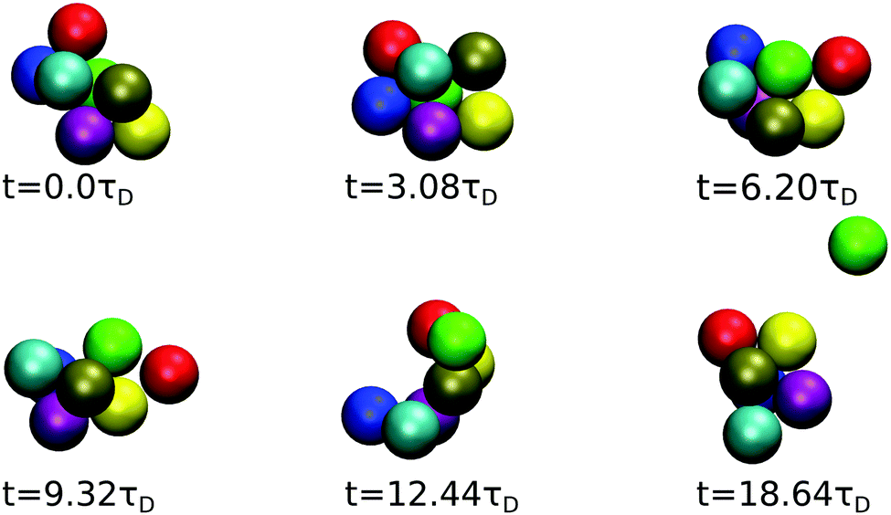Fig. 11 MPC generated time sequence of a cluster consisting of 7 particles for ε = 7 and ρ* = 0.1, tracked until a particle (labeled in green) dissociates.

5 Summary and conclusions

For a representative SALR model dispersion of spherical particles interacting by the generalized Lennard-Jones–Yukawa (LJY) pair potential, static and short-time diffusion properties, and the phase behavior have been determined by using the easy-to-apply BM-PA scheme where HIs are approximately included, and by performing elaborate multiparticle-collision-dynamics simulations, where the effects of many-body HIs are fully accounted for.

We have studied the structural properties via g(r) and S(q), and the equilibrium phase behavior for varying values of the attraction strength (potential well depth) ε and two particle concentrations ρ*. Our phase-state mapping based on alternative criteria invoking the cluster-size distribution function and the IRO peak height and width of S(q), is in accord with a previous study by Mani et al. in ref. 6 on the same model system. A phase transition from the dispersed-fluid to the equilibrium-cluster phase is observed with increasing attraction strength. In the dispersed-fluid phase, the self-consistent ZH scheme gives results for S(q) and g(r) in excellent agreement with MPC simulation data. Likewise for the dispersed-fluid phase, we have shown the good accuracy of the analytic BM-PA results regarding the short-time diffusion function, D(q), by the comparison with corresponding MPC simulation predictions. Thus, the BM-PA scheme allows for the convenient assessment of short-time diffusion properties for dispersed-fluid phase SALR systems.

Using MPC simulations, we have studied the dynamics of LJY systems in the equilibrium-cluster phase, where for the first time the long-range HIs are fully accounted for. The simulations yield for this phase significantly smaller D(q) values as for dispersed-fluid systems. To explore the intra-cluster dynamics, we calculated the dissociation (first passage) time, τ^d_c, for an isolated pair of LJY particles, and compared it with the MPC cluster lifetime, τ_c, for concentrated dispersions. This study is amended by the visualization of the shape changes of a cluster up to the event when a particle is leaving the cluster. The simulations reveal a highly mobil internal cluster dynamics, with pronounced conformational changes within a time span of a few τ_D values. Thus, both, the intra-cluster dynamics and the dynamics of the dispersion as a whole are significantly influenced by many-particle HIs, which are not screened inside flexible clusters. As a consequence, the dynamics of an equilibrium-cluster dispersion cannot be described simply as a polydisperse dispersion of rigid Brownian-cluster objects.

Our results contribute to an improved understanding of the dispersed-particles dynamics in SALR systems. Thereby, the results on the influence of HIs on cluster conformational changes and lifetimes are applicable, on a qualitative level, to general Brownian particle systems, where thermodynamic clusters are formed. As a future technological application, the obtained transport properties can be be used as salient input to a previously developed membrane ultrafiltration model,⁷⁹ in its application to protein solutions under SALR conditions. Furthermore, using MPC simulations, we intend to study, in more detail, the intra-cluster structure and dynamics.

Conflicts of interest

There are no conflicts to declare.

Acknowledgements

J. R. acknowledges support by the International Helmholtz Research School on Biophysics and Soft Matter (IHRS BioSoft). G. N. and J. R. thank M. Heinen (Universidad de Guanajuato, Leon, Mexico) for many helpful discussions.

References

1. A. Stradner, H. Sedgwick, F. Cardinaux, W. C. K. Poon, S. U. Egelhaaf and P. Schurtenberger, Nature, 2004, 432, 492–495.
2. F. Cardinaux, E. Zaccarelli, A. Stradner, S. Bucciarelli, B. Farago, S. U. Egelhaaf, F. Sciortino and P. Schurtenberger, J. Phys. Chem. B, 2011, 115, 7227–7237.
3. P. D. Godfrin, R. Castaneda-Priego, Y. Liu and N. J. Wagner, J. Chem. Phys., 2013, 139, 154904.
4. Y. Liu, L. Porcar, J. Chen, W. R. Chen, P. Falus, A. Faraone, E. Fratini, K. Hong and P. Baglioni, J. Phys. Chem. B, 2011, 115, 7238–7247.
5. P. D. Godfrin, N. E. Valadez-Pérez, R. Castaneda-Priego, N. J. Wagner and Y. Liu, Soft Matter, 2014, 10, 5061–5071.
6. E. Mani, W. Lechner, W. K. Kegel and P. G. Bolhuis, Soft Matter, 2014, 10, 4479–4486.
7. F. Cardinaux, A. Stradner, P. Schurtenberger, F. Sciortino and E. Zaccarelli, Europhys. Lett., 2007, 77, 48004.
8. A. J. Chinchalikar, V. K. Aswal, J. Kohlbrecher and A. G. Wagh, Phys. Rev. E: Stat., Nonlinear, Soft Matter Phys., 2013, 87, 062708.
9. J. A. Bollinger and T. M. Truskett, J. Chem. Phys., 2016, 145, 064903.
10. J. Riest, Dynamics in Colloid and Protein Systems: Hydrodynamically Structured Particles, and Dispersions with Competing Attractive and Repulsive Interactions, Forschungszentrum Jülich GmbH Zentralbibliothek, Jülich, 2016, p. ix, 226.
11. A. Archer and N. Wilding, Phys. Rev. E: Stat., Nonlinear, Soft Matter Phys., 2007, 76, 031501.
12. J. C. F. Toledano, F. Sciortino and E. Zaccarelli, Soft Matter, 2009, 5, 2390.
13. N. E. Valadez-Pérez, R. Castañeda-Priego and Y. Liu, RSC Adv., 2013, 3, 25110–25119.
14. R. Piazza, M. Pierno, S. Iacopini, P. Mangione, G. Esposito and V. Bellotti, Eur. Biophys. J., 2006, 35, 439–445.
15. N. Kovalchuk, V. Starov, P. Langston and N. Hilal, Adv. Colloid Interface Sci., 2009, 147–148, 144–154.
16. S. Yannopoulos and V. Petta, Philos. Mag., 2008, 88, 4161–4168.
17. J. A. Bollinger and T. M. Truskett, J. Chem. Phys., 2016, 145, 064902.
18. J. Riest, G. Nägele, Y. Liu, N. J. Wagner and D. Godfrin, 2017, submitted.
19. M. Roos, M. Ott, M. Hofmann, S. Link, E. Rössler, J. Balbach, A. Krushelnitsky and K. Saalwächter, J. Am. Chem. Soc., 2016, 138, 10365–10372.
20. S. Bucciarelli, J. S. Myung, B. Farago, S. Das, G. A. Vliegenthart, O. Holderer, R. G. Winkler, P. Schurtenberger, G. Gompper and A. Stradner, Sci. Adv., 2016, 2, e1601432.
21. J. Riest and G. Nägele, Soft Matter, 2015, 11, 9273–9280.
22. A. J. Banchio and G. Nägele, J. Chem. Phys., 2008, 128, 104903.
23. M. Heinen, A. J. Banchio and G. Nägele, J. Chem. Phys., 2011, 135, 154504.
24. F. Westermeier, B. Fischer, W. Roseker, G. Grübel, G. Nägele and M. Heinen, J. Chem. Phys., 2012, 137, 114504.
25. C.-C. Huang, G. Gompper and R. G. Winkler, Phys. Rev. E: Stat., Nonlinear, Soft Matter Phys., 2012, 86, 056711.
26. A. Malevanets and R. Kapral, J. Chem. Phys., 1999, 110, 8605.
27. R. Kapral, Adv. Chem. Phys., 2008, 140, 89.
28. G. Gompper, T. Ihle, D. M. Kroll and R. G. Winkler, Adv. Polym. Sci., 2009, 221, 1.
29. S. H. Lee and R. Kapral, J. Chem. Phys., 2004, 121, 11163.
30. M. Hecht, J. Harting, T. Ihle and H. J. Herrmann, Phys. Rev. E: Stat., Nonlinear, Soft Matter Phys., 2005, 72, 011408.
31. J. T. Padding and A. A. Louis, Phys. Rev. E: Stat., Nonlinear, Soft Matter Phys., 2006, 74, 031402.
32. I. O. Götze, H. Noguchi and G. Gompper, Phys. Rev. E: Stat., Nonlinear, Soft Matter Phys., 2007, 76, 046705.
33. M. K. Petersen, J. B. Lechman, S. J. Plimpton, G. S. Grest, P. J. in 't Veld and P. R. Schunk, J. Chem. Phys., 2010, 132, 174106.
34. J. K. Whitmer and E. Luijten, J. Phys.: Condens. Matter, 2010, 22, 104106.
35. T. Franosch, M. Grimm, M. Belushkin, F. M. Mor, G. Foffi, L. Forró and S. Jeney, Nature, 2011, 478, 85.
36. M. Belushkin, R. G. Winkler and G. Foffi, J. Phys. Chem. B, 2011, 115, 14263.
37. S. Poblete, A. Wysocki, G. Gompper and R. G. Winkler, Phys. Rev. E: Stat., Nonlinear, Soft Matter Phys., 2014, 90, 033314.
38. M. Yang, M. Theers, J. Hu, G. Gompper, R. G. Winkler and M. Ripoll, Phys. Rev. E: Stat., Nonlinear, Soft Matter Phys., 2015, 92, 013301.
39. M. Theers, E. Westphal, G. Gompper and R. G. Winkler, Phys. Rev. E, 2016, 93, 032604.
40. A. Malevanets and J. M. Yeomans, Europhys. Lett., 2000, 52, 231–237.
41. K. Mussawisade, M. Ripoll, R. G. Winkler and G. Gompper, J. Chem. Phys., 2005, 123, 144905.
42. C.-C. Huang, R. G. Winkler, G. Sutmann and G. Gompper, Macromolecules, 2010, 43, 10107.
43. M. A. Webster and J. M. Yeomans, J. Chem. Phys., 2005, 122, 164903.
44. J. F. Ryder and J. M. Yeomans, J. Chem. Phys., 2006, 125, 194906.
45. M. Ripoll, R. G. Winkler and G. Gompper, Phys. Rev. Lett., 2006, 96, 188302.
46. S. Frank and R. G. Winkler, Europhys. Lett., 2008, 83, 38004.
47. C. C. Huang, G. Gompper and R. G. Winkler, J. Chem. Phys., 2013, 138, 144902.
48. H. Noguchi and G. Gompper, Proc. Natl. Acad. Sci. U. S. A., 2005, 102, 14159–14164.
49. J. L. Mcwhirter, H. Noguchi and G. Gompper, Proc. Natl. Acad. Sci. U. S. A., 2009, 106, 6039–6043.
50. J. Elgeti, U. B. Kaupp and G. Gompper, Biophys. J., 2010, 99, 1018.
51. J. Hu, M. Yang, G. Gompper and R. G. Winkler, Soft Matter, 2015, 11, 7843.
52. T. Eisenstecken, J. Hu and R. G. Winkler, Soft Matter, 2016, 12, 8316.
53. C. Beenakker and P. Mazur, Phys. A, 1984, 126, 349–370.
54. A. Banchio, J. Gapinski, A. Patkowski, W. Häußler, A. Fluerasu, S. Sacanna, P. Holmqvist, G. Meier, M. Lettinga and G. Nägele, Phys. Rev. Lett., 2006, 96, 138303.
55. R. N. Zia, J. W. Swan and Y. Su, J. Chem. Phys., 2015, 143, 224901.
56. D. Costa, C. Caccamo, J.-M. Bomont and J.-L. Bretonnet, Mol. Phys., 2011, 109, 2845–2853.
57. W. E. J. Verwey and J. T. G. Overbeek, Theory of the Stability of Lyophobic Colloids, Dover Publications, Mineola, NY, 1999.
58. G. Zerah and J.-P. Hansen, J. Chem. Phys., 1986, 84, 2336.
59. Y. Rosenfeld and N. Ashcroft, Phys. Rev. A: At., Mol., Opt. Phys., 1979, 20, 1208–1235.
60. J.-M. Bomont and J.-L. Bretonnet, J. Chem. Phys., 2004, 121, 1548–1552.
61. J.-M. Bomont, J. Chem. Phys., 2003, 119, 11484.
62. J. M. Kim, R. Castañeda-Priego, Y. Liu and N. J. Wagner, J. Chem. Phys., 2011, 134, 064904.
63. G. Nägele, Phys. Rep., 1996, 272, 215–372.
64. C. Beenakker and P. Mazur, Phys. A, 1983, 120, 388–410.
65. C. Beenakker, Phys. A, 1984, 128, 48–81.
66. J. Riest, T. Eckert, W. Richtering and G. Nägele, Soft Matter, 2015, 11, 2821–2843.
67. M. Heinen, F. Zanini, F. Roosen-Runge, D. Fedunová, F. Zhang, M. Hennig, T. Seydel, R. Schweins, M. Sztucki, M. Antalík, F. Schreiber and G. Nägele, Soft Matter, 2012, 8, 1404–1419.
68. M. P. Allen and D. J. Tildesley, Computer Simulation of Liquids, Clarendon Press, Oxford, 1987.
69. T. Ihle and D. M. Kroll, Phys. Rev. E: Stat., Nonlinear, Soft Matter Phys., 2003, 67, 066705.
70. C.-C. Huang, A. Chatterji, G. Sutmann, G. Gompper and R. G. Winkler, J. Comput. Phys., 2010, 229, 168.
71. C.-C. Huang, A. Varghese, G. Gompper and R. G. Winkler, Phys. Rev. E: Stat., Nonlinear, Soft Matter Phys., 2015, 91, 013310.
72. R. B. Jadrich, J. A. Bollinger, K. P. Johnston and T. M. Truskett, Phys. Rev. E: Stat., Nonlinear, Soft Matter Phys., 2015, 91, 042312.
73. F. Sciortino, P. Tartaglia and E. Zaccarelli, J. Phys. Chem. B, 2005, 109, 21942.
74. S. Saw, N. L. Ellegaard, W. Kob and S. Sastry, J. Chem. Phys., 2011, 134, 164506.
75. D. Y. C. Chan and B. Halle, J. Colloid Interface Sci., 1984, 102, 400–409.
76. S. Kim and S. Karrila, Microhydrodynamics: Principles and Selected Applications, Butterworth-Henemann, Boston, 1991.
77. D. J. Jeffrey and Y. Onishi, J. Fluid Mech., 1984, 139, 261–290.
78. R. Jones and R. Schmitz, Phys. A, 1988, 149, 373–394.
79. R. Roa, D. Menne, J. Riest, P. Buzatu, E. K. Zholkovskiy, J. K. G. Dhont, M. Wessling and G. Nägele, Soft Matter, 2016, 12, 4638–4653.

---

Footnote

† These authors contributed equally.

---