
Unfolding dynamics of small peptides biased by constant mechanical forces
Fabian
Knoch
and
Thomas
Speck
 *
*
Institut für Physik, Johannes Gutenberg-Universität Mainz, Staudingerweg 7-9, 55128 Mainz, Germany. E-mail: thomas.speck@uni-mainz.de
First published on 30th October 2017
Abstract
We show how multi-ensemble Markov state models can be combined with constant-force equilibrium simulations. Besides obtaining the unfolding/folding rates, Markov state models allow gaining detailed insights into the folding dynamics and pathways through identifying folding intermediates and misfolded structures. For two specific peptides, we demonstrate that the end-to-end distance is an insufficient reaction coordinate. This problem is alleviated through constructing models with multiple collective variables, for which we employ the time-lagged independent component analysis requiring only minimal prior knowledge. Our results show that combining Markov state models with constant-force simulations is a promising strategy to bridge the gap between simulation and experiments even for medium-sized biomolecules.
Design, System, ApplicationEngineering at the molecular level requires reliable and robust computational tools to predict properties like binding affinities and to efficiently scan large chemical spaces. Given the size of small biomolecules and the time scales involved, these tools inevitably are going to be multiscale methods. We employ discrete Markov state models, which are built from atomistic molecular dynamics simulations but allow faithful sampling of the slowest time scales that are typically far beyond the reach of a single molecular dynamics trajectory. On this time scale, the folding/self-assembly into the native structure occurs, which is required for the particular functionality of the molecules. We demonstrate the feasibility and usefulness of Markov state models to study the folding of single molecules at constant force, an important experimental technique. Here we elucidate the folding pathways of two peptides under an applied external force, but our method is versatile and can be applied to a wide range of bio- and macromolecules. |
I. Introduction
The comprehensive understanding of how proteins fold has been an open question in biomolecular research for the past two decades.1–3 Tackling this problem remains a challenge since the free energy landscape dictating the folding pathways is complex and includes many intermediate and misfolded regions. From the experimental point of view, much insight has been gained by means of force probe spectroscopy,4 especially through atomic force microscopy (AFM)5,6 and optical tweezer experiments.7,8In experiments, probing folding pathways can be realized through applying an extensional force to individual proteins, which is commonly implemented by one of two different protocols: pulling or constant force (force clamp). In pulling experiments, ends are separated with a constant speed or a constant loading rate while recording the force-extension curve. Hence, the protein is driven out of thermal equilibrium but the free energy might be recovered from the fluctuations.9,10 On the other hand, a constant force can be achieved through a feedback loop,4,11,12 which in principle generates an equilibrium ensemble of configurations at that force. Both techniques monitor structural dynamics only along a single reaction coordinate, which means that the interpretation of the data has to rely on theoretical models (see for example ref. 13 and references within).
Computational studies, on the other hand, provide a detailed picture of folding pathways with the full structural dynamics accessible on time scales from nanoseconds to milliseconds. Although millisecond molecular dynamics (MD) trajectories are nowadays affordable for small proteins on supercomputers,14 predicting folding rates requires the computation of trajectories exhibiting many unfolding/folding events. Markov state modeling has tackled this problem successfully for the folding of small proteins15–17 as well as ligand binding kinetics.18 This is achieved by coarse-graining the configuration space of these molecules into discrete sets based on the dynamical information provided by molecular dynamics simulations. Necessarily, the dynamics in this coarse-grained space is stochastic and (approximately) Markovian by virtue of the time scale separation underlying the construction of the discrete sets. One key advantage is that Markov state models (MSMs) can be constructed from many short trajectories, inferring transition rates of processes that are much longer than individual trajectories. Of course, any shortcomings of the input molecular dynamics simulations such as the dependence of certain molecular properties on the chosen force field (e.g., the over-representation of alpha-helical structures51) will still be present in the final MSM.
Despite the modeling advantages and increase in computational power, it is still a challenging task to simulate protein dynamics for more than 100 residues. To connect simulations with force-probe experiments,19–21 molecular dynamics simulations mimic the experimental protocol by either applying a time-dependent harmonic force or a time-independent constant force. The advantage of pulling simulations is that even medium or large-sized proteins can be unfolded in a reasonable amount of time, though pulling velocities commonly differ by orders of magnitude from experimental velocities. Theoretical and experimental studies22,23 show, however, that folding pathways are dependent on pulling velocities, which makes direct comparison with experiments challenging. Another drawback is that the protein and its environment are not in thermodynamic equilibrium. More precisely, through the driving, they do not reach a steady state and hence cannot be described by Boltzmann's statistics. In constant-force simulations,24–26 on the other hand, a time-independent constant biasing force is applied, allowing the expression of all molecular interactions through a Hamiltonian operator. Constant-force simulations thus follow equilibrium statistical mechanics, enabling the construction of equilibrium MSMs while still accelerating the protein dynamics. In this study, we illustrate the application of equilibrium Markov state modeling to constant-force simulations for two specific peptides.
II. Methods
A. Markov state modeling and transition-based reweighting
The transition-based reweighting method (TRAM) is an approach to connect multiple equilibrium ensembles, moving beyond well-established approaches such as the weighted histogram analysis method.27 Its main advantage is that rare events in one ensemble can become less rare in another ensemble. TRAM exploits information about the probability distribution sampled in these “less rare” ensembles to improve estimations of rare events. Here we only give a brief summary of the method and the readers are referred for a detailed description to the original publications.28,29We consider a system effectively described by a one-dimensional collective variable (CV) r (the generalization to multi-dimensional CVs is straightforward). Defining the dimensionless potential of the mean force as βU(r) with β−1 = kBT, the probability distribution is given by the Boltzmann factor
| p(r) = e−βU(r)/Z, | (1) |
| pk(r) = p(r)e−Bk(r)/Zk, | (2) |
 .
.
The first step is to discretize the CV r into finite, non-overlapping cells (or centroids) with Ri being the ith centroid. The space-continuous MD trajectories are mapped onto all Ri centroids returning a Markov chain. To infer dynamical information, all observed transitions between states Ri → Rj are counted by ckij. Finally, to estimate the entries tkij of the transition matrices, a maximum likelihood approach is employed, which estimates all entries tkij based on the observed transition counts ckij,
 | (3) |
We emphasize that eqn (3) is valid for every ensemble. Equilibrium dynamics obeys detailed balance pkitkij = pkjtkji, which is used to constrain the maximization of eqn (3). This constraint enforces the stationary state of the MSM to correspond to thermal equilibrium.30
To infer information from multiple ensembles, we express the stationary probability of centroid Ri
 | (4) |
| Zki = Zk∫Ripk(r)dr | (5) |
Connecting eqn (2) with eqn (3) and exploiting the local equilibrium conditions in eqn (4), the TRAM maximum likelihood function follows as
 | (6) |
B. Constructing collective variables
A key feature in order to construct MSMs is to have a “good” phase space discretization (fine-graining) of the system. Even with the availability of efficient clustering algorithms, e.g., k-means or k-centers, taking all degrees of freedom of a biomolecular system into account will most probably not result in a meaningful fine-grained discretization of the phase space. The usual procedure is to neglect all momenta, positions of solvent atoms, and to use relative coordinates (distances, angles, etc.) instead of absolute positions, as most MD simulations are conducted under periodic boundary conditions. To distinguish the set of chosen coordinates from the full phase space, it is often referred to as the configuration space, a convention we adopt in this study.To study conformational changes of peptides, a reasonable set of coordinates is given by the distances between Cα atoms, still spanning a high-dimensional configuration space. To further reduce the complexity of the configuration space, we employ the time-lagged independent component analysis (TICA).32 In addition to spatial information, TICA uses temporal information through computing time-lagged covariance matrices ∑(τ) = (σij(τ)) and solving the generalized eigenvalue problem
∑(τ)U = ![[thin space (1/6-em)]](https://www.rsc.org/images/entities/char_2009.gif) ∑(0)UΛ ∑(0)UΛ | (7) |
C. Simulations
For all MD simulations, we employ the Gromacs 5.1.2 software package.33 All simulations are conducted in the NPT ensemble with the temperature set to 300 K, for which the velocity-rescaling34 thermostat with τT = 1 ps is employed. For isotropic pressure coupling, we use the Parrinello–Rahman35 barostat with τp = 2 ps and compressibility of 4.5 × 10⁻⁵ bar−1. Long-range electrostatics are treated employing particle mesh Ewald summation with cubic interpolation and a Fourier grid spacing of 0.16 nm. All short-ranged interactions are cutoff at 1.0 nm and all hydrogen-involving covalent bonds are restrained by the LINCS algorithm.36 The time step is set to 2 fs.III. Results
A. Alpha-peptide
As a first example, we choose the well-studied peptide deca-alanine, which is an alpha-helical forming model system.37,38 To study how the folding/unfolding dynamics changes, a constant-force is imposed between the center of mass of the N-terminus and the center of mass of the C-terminus of the peptide, the distance between which defines the end-to-end distance of the peptide. We create 48 independent simulations from multiple starting configurations randomly selected from a 50 ns trajectory for four different force magnitudes f = {0, 5, 10, 15} kJ mol−1 nm−1 [f = {0, 8.3, 16.6, 24.9} pN], accumulating a total of 2–2.5 μs per force. For reference, harvesting this data has taken approx. 2500 CPU hours. The molecular interactions of deca-alanine are described by the CHARMM22/CMAP39 force field, while we employ TIP3P40 water to model solvent interactions. The peptide is positioned in a cubic box with a 7.2 nm box length and periodic boundary conditions, solvated by ≃12000 water molecules. To ensure that every trajectory is properly equilibrated, we discard its first 2 ns.
To construct a reasonable set of CVs, we employ the TICA algorithm. As original configuration space representation serving as the input for TICA, we choose all Cα pair distances which are separated by at least two residues and, additionally, all native hydrogen bond distances between donor (nitrogen) and acceptor (oxygen) atoms that stabilize alpha-helical structures. More precisely, we use the distance between C![[double bond, length as m-dash]](https://www.rsc.org/images/entities/char_e001.gif) O of the ith residue and N–H of the (i + 4)th residue. We compute the TICA time scale −τTICA/log(λTICA) for multiple lag times τTICA (see Fig. 1a). We select τTICA = 5 ns for the final representation since it is the shortest lag time for which the slowest implied TICA time scale is approximately independent of the lag time. Moreover, the number of effective TICA components recovering at least 90% of the kinetic variance, i.e.,
O of the ith residue and N–H of the (i + 4)th residue. We compute the TICA time scale −τTICA/log(λTICA) for multiple lag times τTICA (see Fig. 1a). We select τTICA = 5 ns for the final representation since it is the shortest lag time for which the slowest implied TICA time scale is approximately independent of the lag time. Moreover, the number of effective TICA components recovering at least 90% of the kinetic variance, i.e.,  , drops down to four.
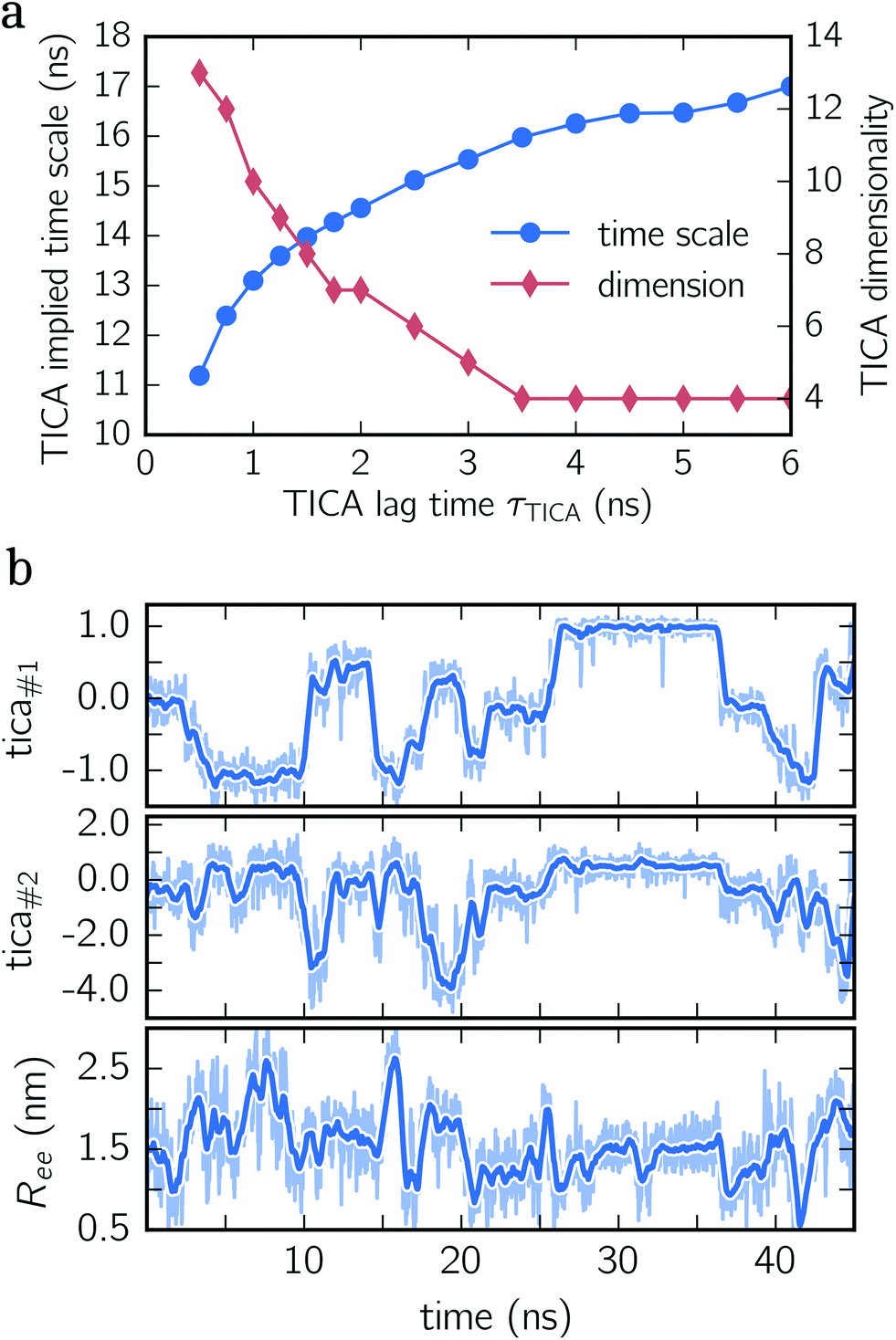 | ||
| Fig. 1 TICA analysis for deca-alanine. (a) Implied TICA time scale and the number of effective TICA components are shown for different lag times τTICA. (b) Exemplary times series of deca-alanine. All three panels show the same time series projected onto the first TICA component (upper panel), the second TICA component (center panel) and end-to-end distance (lower panel). Detailed time series are illustrated by shaded lines, whereas thick lines represent moving averages. | ||
For this 34-dimensional configuration space, we keep the first four TICA components exhibiting a cumulative kinetic variance >92%. Together with the end-to-end distance, the 5-dimensional reduced configuration space is discretized employing the k-means clustering algorithm with 300 clusters. For the TICA input, we use only trajectories for f = 5 kJ mol−1 nm−1 since TICA computes its dominant components based on the information stored in the time-lagged covariance matrix (see eqn (7)) and thus an input mixed from different constant-force ensembles would lead to inferior results for the independent components. However, all trajectories serve as the input for the k-means clustering algorithm. Because the output of the k-means algorithm depends on the starting configuration of centroids (zeroth iteration), we perform the clustering with 50 different randomly selected configurations and select the discretization exhibiting the smallest error. We verified that the best three discretizations do not show any qualitative difference.
Regarding the choice of the initial configuration space representation (Cα distances and hydrogen bond distances), all of these coordinates, including the biasing coordinate (end-to-end distance), come with a distance metric, which improves the clustering results of the k-means algorithm and the subsequent space-discretization of trajectories. Note that in the study of Jo et al.38 the authors pursue a similar approach, though only using the Cα distances.
After mapping the trajectories of all constant-force ensembles onto the reduced configuration space and counting all observed transitions, we use TRAM with a lag time of τTRAM = 4 ns returning a fine-grained MSM for every ensemble containing 300 micro states (clusters). The selected lag time is the shortest for which the slowest implied time scale, i.e., −τTRAM/log(λTRAM), is approximately constant (data not shown) for all ensembles. As a means of error estimation, we split the 48 trajectories per applied external force into six independent sets and repeat the TRAM estimation for each set individually. In the following analysis, error bars correspond to the standard error computed from these six sets. If not shown, error bars are smaller than the marker size.
In Fig. 1b, an exemplary time series of the first two TICA components and the end-to-end distance for deca-alanine is shown. First, note that more than two states are involved which can be clearly seen in the time series of the first TICA component (upper panel) illustrated by jumps between plateaus (metastable states) with different amplitudes. The time series of the second TICA component offers less plateaus with more fluctuations (see the shaded time series), while for the time series of the end-to-end distance (lower panel), plateaus are insufficiently resolved. Additionally, fluctuations of the end-to-end distance are much stronger for the TICA components shown. The comparison of all three time series illustrates that for deca-alanine both TICA components are better suited as CVs than the end-to-end distance of the peptide.
logpi. Fig. 2a (upper panel) shows the free energy of every micro-state with (f = 10 kJ mol−1 nm−1) and without constant-force bias (f = 0 kJ mol−1 nm−1) exhibiting its global minimum at fmin ≈ 1.6 nm corresponding to the alpha-helical structure. Although the position of the minimum is identical for both ensembles, their free energy landscapes differ drastically. While for f = 0 kJ mol−1 nm−1 the free energy for shorter end-to-end distances is lower than for elongated configurations, the opposite applies for f = 10 kJ mol−1 nm−1 where the free energy of elongated configurations is almost as low as for folded ones. Furthermore, the maximum free energy difference is up to 25% higher for the unbiased ensemble.
 | ||
| Fig. 2 Deca-alanine. (a) Scatter plot of free energy against the end-to-end distance of every individual centroid for f = 0 kJ mol−1 nm−1 (upper panel) and f = 10 kJ mol−1 nm−1 (lower panel). Points (centroids) are colored corresponding to their metastable set, as shown in (c). (b) The free energy landscape integrated along the end-to-end distance (bin size = 0.2 nm) is shown for the unbiased dynamics (upper panel) and for all ensembles (lower panel) f = {0, 5, 10, 15} kJ mol−1 nm−1. Blue and green points (upper panel) follow from an independent Markov state modeling approach and from direct sampling (see the main text), respectively. Shaded regions indicate error bars, if larger than the marker. (c) Configuration space projected onto the first and second TICA components (upper panel) and onto the first TICA component and the end-to-end distance (lower panel). Circles correspond to centroids discretizing configuration space (fine-graining). Colored circles represent configurations belonging to metastable sets with different colors corresponding to different metastable sets. An exemplary snapshot for every metastable configuration is shown and related to its position in the configuration space. Gray circles represent transition states which are not assigned to any metastable set. (d) Folding and unfolding rates (inverse mean-first passage times between light blue and green states) of deca-alanine for all constant-force ensembles. (e) Occupation probability of misfolded configurations for biased/unbiased ensembles. Colors match the metastable sets shown in (c). The inset shows the total percentage to occupy a misfolded state. | ||
For a better comparison with previous studies (see the Discussion section), we integrate out all dimensions except the end-to-end distance. The results for all ensembles are shown in Fig. 2c (lower panel) for which the probability distributions are binned with a bin size of 0.2 nm. For f = {0, 5, 10} kJ mol−1 nm−1, the global minimum is located at the same position as in Fig. 2a. However, for f = 15 kJ mol−1 nm−1, the global minimum is shifted (≃2.5 nm) toward the elongated configurations.
Moreover, we use this integrated free energy profile to verify the TRAM approach (for an in-depth benchmark see ref. 29). To this end, we conduct 48 additional (50 ns each) MD simulations for the unbiased ensemble and determine the integrated free energy (along the end-to-end distance) by constructing a “regular” MSM on the same configuration space discretization (τMSM = 4 ns and maximum likelihood estimator, see eqn (3)) and by computing the histogram over all trajectory frames. The obtained free energy profiles agree well with the results obtained from TRAM (see Fig. 2b).
In Fig. 2c, two projections of the discretized configuration space are shown along the first two TICA components as well as along the first TICA component and the end-to-end distance. While different colors indicate different metastable sets, gray centroids belong to transition states. One issue arises here: although the PCCA+ suggests 6 metastable sets, we manually separate stretched configurations (configurations in which all residues are almost linearly aligned, light blue colored set) from unfolded/weakly coiled configurations (orange set) as the former can be clearly identified by their end-to-end distance. PCCA+ does not detect stretched configurations automatically because they are temporally not well separated from the remaining unfolded configurations (orange set). These remaining unfolded configurations are weakly coiled along the centered residues, while outer residues can fluctuate freely. Large fluctuations of the outer residues can lead to hairpin-like structures which are stabilized by hydrogen bonds of the outer residues (yellow set). Hairpin-like structures are misfolded configurations acting as traps which slow down the folding process. Other misfolded configurations are detected by the red, magenta, dark blue and cyan colored sets. All of these misfolded configurations have a thing in common – that at some residues, the helical structure is disturbed, e.g., coiled in the wrong direction and stabilized by hydrogen bonds different from the ones guaranteeing the correct alpha-helical structure. Moreover, these misfolded structures act as “dead ends” in the folding process, i.e., to reach the correctly folded helical structure the peptide has to reverse the “misfolding step” first and pass through folding intermediates (orange colored configurations). Lastly, the green metastable set represents correctly folded configurations, that is, the dihedral angles formed by the inner residues are in the alpha helical configuration.
Knowing the probability distribution for all ensembles, we determine the cumulated probability of populating misfolded states (cyan, yellow, dark blue and magenta colored states in Fig. 2c). As show in Fig. 2e, all probabilities decrease drastically with increasing biasing force f. The sum over all misfolded probabilities (inset) equals approx. 17% without bias and vanishes (less than 1%) for f = 15 kJ mol−1 nm−1. Individually, cyan colored configurations exhibit the largest population probability for f = 0 kJ mol−1 nm−1 (approx. 8%), followed by yellow and magenta colored configurations, with red and dark blue colored states being less important. For f = {5, 10} kJ mol−1 nm−1, the order is partially disturbed and lost (or not significant) for f = 15 kJ mol−1 nm−1.
Finally, folding/unfolding rates of deca-alanine are determined by computing inverse mean-first passage times (MFPTs) between correctly folded (green) and stretched (light blue) configurations. Fig. 2d shows both rates for all ensembles ranging from 7 × 10⁻⁴–4 × 10⁻² ns−1 (unfolding) and from 2 × 10⁻²–3 × 10⁻³ ns−1 (folding).
B. Beta-peptide
For the second example, we choose the beta-peptide β-HALA8, which is an octamer containing eight alanine residues. The biasing force is applied along the vector connecting the Cβ atoms of the first and last residues, which we refer to as the end-to-end distance of the peptide. The peptide is described by the GROMOS 53A6 force field.42 Periodic boundary conditions are imposed on the cubic simulation box (7 nm box length), which is filled with ≃12000 water molecules. We use the SPC water model43 and the GROMOS 53A6 force field in order to make our results comparable to previous studies.44 We create 48 trajectories from different starting configurations randomly selected from a 50 ns trajectory, accumulating 2–2.5 μs of the constant-force ensembles f = {0, 2, 5, 10} kJ mol−1 nm−1 [f = {0, 4.15, 8.3, 16.6} pN]. Collecting the data has taken approx. 2500 CPU hours.
As an initial configuration space representation, we select all Cβ distances excluding the two closest neighbors, as well as all hydrogen bond forming donor–acceptor distances that stabilize the beta-helical structure. More precisely, the distance between CO of the ith residue and N–H of the (i − 2)th residue is chosen. This 21-dimensional space is reduced by TICA to three effective dimensions (cumulative kinetic variance >95%), for which we select the lag time τTICA = 2 ns due to a similar reasoning to that for deca-alanine. Including the end-to-end distance, a reduced 4-dimensional configuration space representation is then discretized into 300 micro-states employing the k-means clustering algorithm. Again, we use for TICA only the trajectories belonging to f = 5 kJ mol−1 nm−1, while all trajectories serve as an input for the k-means algorithm. Next, we map all trajectories onto the discretized configuration space and estimate the transition matrices for all ensembles by employing TRAM with a lag time τTRAM = 0.6 ns, due to a lag time analysis (data not shown). Similar to the deca-alanine example, we compute error bars by splitting the 48 trajectories per external force into six independent sets, repeating the analysis for every set, and determining the standard error. If not shown, error bars are smaller than the marker size.
 | ||
| Fig. 3 Beta-alanine. (a) Configuration space projection of the first and second TICA components (upper panel) as well as the first TICA component and end-to-end distance (lower panel) for f = 0 kJ mol−1 nm−1. Colored circles indicate centroids belonging to different metastable sets. Gray circles illustrate transition states that do not belong to any metastable set. (b) Reactive transition network of unfolding pathways is shown for the unbiased dynamics. Each snapshot represents its metastable set [cf. (a)] while arrows indicate the direction of net transitions and their thickness the transition frequency. (c) The same reactive transition network as in (b) but for f = {5, 10, 15} kJ mol−1 nm−1. (d) Scatter plot of free energies against the end-to-end distance for f = 0 kJ mol−1 nm−1. Points (centroids) are colored corresponding to their metastable set, as shown in (a). (e) Free energy landscape projected and integrated along the first TICA component for f = 0 kJ mol−1 nm−1 (upper panel) and for all ensembles f = {0, 2, 5, 10} kJ mol−1 nm−1 (lower panel). Shaded regions indicate error bars, if larger than the marker. All free energy landscapes are rescaled with respect to the minimum for f = 0 kJ mol−1 nm−1. An exemplary snapshot is shown illustrating structures corresponding to the circled point of the free energy landscape for f = 10 kJ mol−1 nm−1. (f) Folding/unfolding rates for all ensembles. | ||
Next, we quantify the importance of folding intermediates by determining the unfolding pathways of the peptide. To this end, we employ a discrete transition path theory46 by identifying and weighting pathways starting from folded and ending with stretched configurations. In Fig. 3b, we show the transition network for the unbiased ensemble, where metastable sets are represented by an exemplary snapshot and enumerated by colored labels with colors matching the colors used in Fig. 3a. The arrows point in the direction of the reactive flux with their width indicating the relative importance of its transition (the thicker, the more important). For example, the transition from state 1 to 4 illustrates that between 10% and 25% of all transition pathways – connecting folded and stretched configurations – run along this transition. The main contribution is given by pathways containing folding intermediates, while structures coiled at the N-terminus (dark blue) are less important. Interestingly, pathways including misfolded configurations do not contribute (<5%) to the unfolding pathways, indicating that these states act as kinetic traps. A similar picture is obtained when applying the same analysis to the constant-force ensembles shown in Fig. 3c, although slight differences appear. For f = {5, 10} kJ mol−1 nm−1, for instance, the transition from 1 → 2 vanishes. However, a new transition from 4 → 1 appears or rather becomes more dominant. Moreover, the most dominant pathway changes from 1 → 3 → 5 for f = {0, 2} kJ mol−1 nm−1 to 1 → 4 → 3 → 5 for f = {5, 10} kJ mol−1 nm−1. Numerical values for all shown transitions are presented in Table 1.
| # Transition | f = 0 | f = 2 | f = 5 | f = 10 |
|---|---|---|---|---|
| 1 → 2 | 8 ± 1 | 10 ± 1 | — | — |
| 1 → 3 | 45 ± 3 | 42 ± 2 | 46 ± 2 | 32 ± 4 |
| 1 → 4 | 31 ± 3 | 34 ± 3 | 42 ± 2 | 54 ± 2 |
| 2 → 3 | 8 ± 1 | 10 ± 2 | 7 ± 1 | 11 ± 2 |
| 3 → 5 | 74 ± 1 | 72 ± 2 | 74 ± 2 | 68 ± 1 |
| 4 → 2 | — | — | 8 ± 1 | 10 ±1 |
| 4 → 3 | 20 ± 2 | 22 ± 1 | 23 ± 1 | 26 ± 4 |
| 4 → 5 | 10 ± 1 | 11 ± 1 | 10 ± 1 | 18 ± 3 |
IV. Discussion
A. Choice of collective variables
For both examples, we showed that the end-to-end distance is not a well-suited CV since many metastable sets cannot be distinguished solely by the end-to-end distance (cf. lower panels of Fig. 2c and 3a) requiring an orthogonal CV. In the study of Hazel et al.,37 the authors came to a similar conclusion. In particular, they investigated the folding dynamics for deca-alanine under vacuum and in water, where a second CV describing the alpha-helical content is employed yielding better insight into the folding/unfolding pathways. Here we employed TICA as a semi-automated routine creating a minimal set of orthogonal CVs being able to accurately describe the configuration space. Besides the alpha-helical/beta-helical structure, the chosen TICA space is able to resolve misfolded configurations (see upper panels of Fig. 2c and 3a).Although the dihedral angles spanned by every residue represent a well-tested set of CVs,47 our results show that the Cα/Cβ and hydrogen bond distances employed here yield an equivalently good description. The results of the study of Vitalini et al.,48 in which the authors explored the (unbiased) helix–coil transition for deca-alanine for different force fields by constructing MSMs from a discretized dihedral space, are in good agreement with our results; in particular when comparing the slowest implied time scales and the shortest lag time at which the implied time scales become lag time independent.
B. Free energy landscapes and metastable configurations
To estimate the transition times between two different types of states, e.g., stretched and folded configurations, a commonly used method is to determine the potential of the mean force (PMF) by umbrella sampling methods.49 Therefore, many umbrella potentials are placed along one or multiple CVs. Using more than one CV becomes quickly very expensive, making it very difficult to accurately determine a PMF when a “good” CV is not known beforehand or does simply not exist. However, the more complex (larger) a peptide/protein is, the higher the CV space becomes if essential energy barriers should not be missed. Furthermore, we want to emphasize that umbrella sampling along only the end-to-end distance is prone to errors as it is easy to miss certain metastable sets. For example, in Fig. 2c, the hairpin (yellow) and wrongly coiled (cyan) structures share a common end-to-end distance. The barrier between both states is, however, very large because the hairpin structure has to be extended first.To compare the unbiased PMF of deca-alanine with previous studies, we compute the PMF along the end-to-end distance (see Fig. 2b). While its global minimum is found at 1.46 nm in ref. 37 and at around 1.4 nm in ref. 38, we find it at 1.6 nm, which agrees well when regarding the different definitions of the end-to-end distance. The general form of the PMF is in very good agreement with ref. 38, but differs from ref. 37 due to the different force field (CHARMM36 (ref. 50)) used. This difference stems from the fact that the CHARMM22/CMAP force field is over-stabilizing the alpha-helical structure.51
The PMF along the first TICA component of beta-alanine (cf.Fig. 3e) reveals three stable regions corresponding to: folded structures, an intermediate, and weakly folded structures; with the latter being the most dominant region. When only considering the end-to-end distance (Fig. 3d), the integrated PMF decreases monotonically (data not shown) in agreement with the results obtained by Uribe et al.44 Moreover, in their study, the authors employed force-probe MD simulations separating the N- and C-termini with a constant velocity. By means of force-extension curves and hydrogen bond analyses, the authors concluded that the unfolding pathway includes two intermediates before obtaining a fully stretched peptide. We identify these intermediates with the magenta and orange colored sets shown in Fig. 3a and b. These findings are further supported by the reactive flux analysis as illustrated in Fig. 3b and c. Imposing a constant force shifts the weight of transitions pathways. Specifically, the transition 1 → 4 becomes more frequent while the transition 1 → 3 becomes less frequent with increasing bias. In other words, when applying a larger force, it is more likely to pass magenta colored states than without an applied force.
The additional minimum in the PMF for f = 10 kJ mol−1 nm−1 (lower panel Fig. 3e), however, suggests that the free energy landscape is drastically modified by the biasing force. To elucidate the mechanism causing the additional minimum, we visualize an exemplary configuration for tica#1 ≃ −0.7 exhibiting a low free energy. The snapshot shown in Fig. 3e illustrates that the outer residues are stretched while the inner residues are stabilized by hydrogen bonds.
Conflicts of interest
There are no conflicts of interest to declare.Acknowledgements
We thank G. Diezemann for discussions and for suggesting the beta-peptide. We acknowledge the DFG for financial support through the TRR 146 Collaborative Research Center (project A7). The authors gratefully acknowledge the computing time granted on the supercomputer Mogon at Johannes Gutenberg University Mainz (hpc.uni-mainz.de).Notes and references
- A. Nicholls, K. A. Sharp and B. Honig, Protein folding and association: insights from the interfacial and thermodynamic properties of hydrocarbons, Proteins: Struct., Funct., Bioinf., 1991, 11, 281–296 CrossRef CAS PubMed.
- K. A. Dill, S. Bromberg, K. Yue, H. S. Chan, K. M. Ftebig, D. P. Yee and P. D. Thomas, Principles of protein folding: a perspective from simple exact models, Protein Sci., 1995, 4, 561–602 CrossRef CAS PubMed.
- C. M. Dobson, Protein folding and misfolding, Nature, 2003, 426, 884–890 CrossRef CAS PubMed.
- G. Žoldák and M. Rief, Force as a single molecule probe of multidimensional protein energy landscapes, Curr. Opin. Struct. Biol., 2013, 23, 48–57 CrossRef PubMed.
- M. Rief, M. Gautel, F. Oesterhelt, J. M. Fernandez and H. E. Gaub, Reversible unfolding of individual titin immunoglobulin domains by AFM, Science, 1997, 276, 1109–1112 CrossRef CAS PubMed.
- M. Carrion-Vazquez, A. F. Oberhauser, S. B. Fowler, P. E. Marszalek, S. E. Broedel, J. Clarke and J. M. Fernandez, Mechanical and chemical unfolding of a single protein: a comparison, Proc. Natl. Acad. Sci. U. S. A., 1999, 96, 3694–3699 CrossRef CAS.
- M. S. Z. Kellermayer, S. B. Smith, H. L. Granzier and C. Bustamante, Folding–unfolding transitions in single titin molecules characterized with laser tweezers, Science, 1997, 276, 1112–1116 CrossRef CAS PubMed.
- C. Cecconi, E. A. Shank, C. Bustamante and S. Marqusee, Direct observation of the three-state folding of a single protein molecule, Science, 2005, 309, 2057–2060 CrossRef CAS PubMed.
- G. Hummer and A. Szabo, Free energy reconstruction from nonequilibrium single-molecule pulling experiments, Proc. Natl. Acad. Sci. U. S. A., 2001, 98, 3658 CrossRef CAS PubMed.
- D. Collin, F. Ritort, C. Jarzynski, S. B. Smith, I. Tinoco and C. Bustamante, Verification of the Crooks fluctuation theorem and recovery of RNA folding free energies, Nature, 2005, 437, 231 CrossRef CAS PubMed.
- W. J. Greenleaf, M. T. Woodside, E. A. Abbondanzieri and S. M. Block, Passive all-optical force clamp for high-resolution laser trapping, Phys. Rev. Lett., 2005, 95, 208102 CrossRef PubMed.
- J. Schönfelder, R. Perez-Jimenez and V. Muñoz, A simple two-state protein unfolds mechanically via multiple heterogeneous pathways at single-molecule resolution, Nat. Commun., 2016, 7, 11777 CrossRef PubMed.
- O. K. Dudko, G. Hummer and A. Szabo, Theory, analysis, and interpretation of single-molecule force spectroscopy experiments, Proc. Natl. Acad. Sci. U. S. A., 2008, 105, 15755–15760 CrossRef CAS PubMed.
- K. Lindorff-Larsen, S. Piana, R. O. Dror and D. E. Shaw, How fast-folding proteins fold, Science, 2011, 334, 517–520 CrossRef CAS PubMed.
- F. Noé, C. Schütte, E. Vanden-Eijnden, L. Reich and T. Weikl, Constructing the equilibrium ensemble of folding pathways from short off-equilibrium simulations, Proc. Natl. Acad. Sci. U. S. A., 2009, 106, 19011 CrossRef PubMed.
- V. A. Voelz, G. R. Bowman, K. Beauchamp and V. S. Pande, Molecular simulation of ab initio protein folding for a millisecond folder ntl9 (1-39), J. Am. Chem. Soc., 2010, 132, 1526–1528 CrossRef CAS PubMed.
- G. R. Bowman and V. S. Pande, Protein folded states are kinetic hubs, Proc. Natl. Acad. Sci. U. S. A., 2010, 107, 10890–10895 CrossRef CAS PubMed.
- N. Plattner and F. Noé, Protein conformational plasticity and complex ligand-binding kinetics explored by atomistic simulations and Markov models, Nat. Commun., 2015, 6, 7653 CrossRef PubMed.
- H. Grubmüller, B. Heymann and P. Tavan, Ligand binding: molecular mechanics calculation of the streptavidin–biotin rupture force, Science, 1996, 997–999 Search PubMed.
- H. Lu, B. Isralewitz, A. Krammer, V. Vogel and K. Schulten, Unfolding of titin immunoglobulin domains by steered molecular dynamics simulation, Biophys. J., 1998, 75, 662–671 CrossRef CAS PubMed.
- D. deSancho and R. B. Best, Reconciling intermediates in mechanical unfolding experiments with two-state protein folding in bulk, J. Phys. Chem. Lett., 2016, 7, 3798–3803 CrossRef CAS PubMed.
- Z. T. Yew, M. Schlierf, M. Rief and E. Paci, Direct evidence of the multidimensionality of the free-energy landscapes of proteins revealed by mechanical probes, Phys. Rev. E: Stat., Nonlinear, Soft Matter Phys., 2010, 81, 031923 CrossRef PubMed.
- F. Rico, L. Gonzalez, I. Casuso, M. Puig-Vidal and S. Scheuring, High-speed force spectroscopy unfolds titin at the velocity of molecular dynamics simulations, Science, 2013, 342, 741–743 CrossRef CAS PubMed.
- E. Paci and M. Karplus, Forced unfolding of fibronectin type 3 modules: an analysis by biased molecular dynamics simulations, J. Mol. Biol., 1999, 288, 441–459 CrossRef CAS PubMed.
- M. Sotomayor and K. Schulten, Single-molecule experiments in vitro and in silico, Science, 2007, 316, 1144–1148 CrossRef CAS PubMed.
- R. B. Best and G. Hummer, Protein folding kinetics under force from molecular simulation, J. Am. Chem. Soc., 2008, 130, 3706–3707 CrossRef CAS PubMed.
- S. Kumar, J. M. Rosenberg, D. Bouzida, R. H. Swendsen and P. A. Kollman, The weighted histogram analysis method for free-energy calculations on biomolecules. i. the method, J. Comput. Chem., 1992, 13, 1011–1021 CrossRef CAS.
- A. S. J. S. Mey, H. Wu and F. Noé, xtram: Estimating equilibrium expectations from time-correlated simulation data at multiple thermodynamic states, Phys. Rev. X, 2014, 4, 041018 Search PubMed.
- H. Wu, F. Paul, C. Wehmeyer and F. Noé, Multiensemble Markov models of molecular thermodynamics and kinetics, Proc. Natl. Acad. Sci. U. S. A., 2016, 113, E3221–E3230 CrossRef CAS PubMed.
- J.-H. Prinz, H. Wu, M. Sarich, B. Keller, M. Senne, M. Held, J. D. Chodera, C. Schütte and F. Noé, Markov models of molecular kinetics: Generation and validation, J. Chem. Phys., 2011, 134, 174105 CrossRef PubMed.
- M. K. Scherer, B. Trendelkamp-Schroer, F. Paul, G. Perez-Hernandez, M. Hoffmann, N. Plattner, C. Wehmeyer, J.-H. Prinz and F. Noé, PyEMMA 2: A Software Package for Estimation, Validation, and Analysis of Markov Models, J. Chem. Theory Comput., 2015, 11, 5525–5542 CrossRef CAS PubMed.
- G. Pérez-Hernández, F. Paul, T. Giorgino, G. DeFabritiis and F. Noé, Identification of slow molecular order parameters for Markov model construction, J. Chem. Phys., 2013, 139, 015102 CrossRef PubMed.
- M. J. Abraham, T. Murtola, R. Schulz, S. Páll, J. C. Smith, B. Hess and E. Lindahl, Gromacs: High performance molecular simulations through multi-level parallelism from laptops to supercomputers, SoftwareX, 2015, 1, 19–25 CrossRef.
- G. Bussi, D. Donadio and M. Parrinello, Canonical sampling through velocity rescaling, J. Chem. Phys., 2007, 126, 014101 CrossRef PubMed.
- M. Parrinello and A. Rahman, Polymorphic transitions in single crystals: A new molecular dynamics method, J. Appl. Phys., 1981, 52, 7182–7190 CrossRef CAS.
- B. Hess, H. Bekker, H. J. C. Berendsen and J. G. E. M. Fraaije, Lincs: a linear constraint solver for molecular simulations, J. Comput. Chem., 1997, 18, 1463–1472 CrossRef CAS.
- A. Hazel, C. Chipot and J. C. Gumbart, Thermodynamics of deca-alanine folding in water, J. Chem. Theory Comput., 2014, 10, 2836–2844 CrossRef CAS PubMed.
- S. Jo, D. Suh, Z. He, C. Chipot and B. Roux, Leveraging the information from Markov state models to improve the convergence of umbrella sampling simulations, J. Phys. Chem. B, 2016, 120, 8733–8742 CrossRef CAS PubMed.
- A. D. MacKerell, M. Feig and C. L. Brooks, Extending the treatment of backbone energetics in protein force fields: Limitations of gas-phase quantum mechanics in reproducing protein conformational distributions in molecular dynamics simulations, J. Comput. Chem., 2004, 25, 1400–1415 CrossRef CAS PubMed.
- W. L. Jorgensen, J. Chandrasekhar, J. D. Madura, R. W. Impey and M. L. Klein, Comparison of simple potential functions for simulating liquid water, J. Chem. Phys., 1983, 79, 926–935 CrossRef CAS.
- S. Röblitz and M. Weber, Fuzzy spectral clustering by PCCA+: application to Markov state models and data classification, Adv. Data Anal. Classif., 2013, 7, 147–179 CrossRef.
- C. Oostenbrink, A. Villa, A. E. Mark and W. F. VanGunsteren, A biomolecular force field based on the free enthalpy of hydration and solvation: the GROMOS force-field parameter sets 53a5 and 53a6, J. Comput. Chem., 2004, 25, 1656–1676 CrossRef CAS PubMed.
- H. J. C. Berendsen, J. R. Grigera and T. P. Straatsma, The missing term in effective pair potentials, J. Phys. Chem., 1987, 91, 6269–6271 CrossRef CAS.
- L. Uribe, J. Gauss and G. Diezemann, Comparative study of the mechanical unfolding pathways of α- and β-peptides, J. Phys. Chem. B, 2015, 119, 8313–8320 CrossRef CAS PubMed.
- We separate stretched configurations from unfolded configurations according to their end-to-end distance.
- J.-H. Prinz, B. Keller and F. Noé, Probing molecular kinetics with Markov models: metastable states, transition pathways and spectroscopic observables, Phys. Chem. Chem. Phys., 2011, 13, 16912–16927 RSC.
- A. Altis, M. Otten, P. H. Nguyen, R. Hegger and G. Stock, Construction of the free energy landscape of biomolecules via dihedral angle principal component analysis, J. Chem. Phys., 2008, 128, 06B620 CrossRef PubMed.
- F. Vitalini, A. S. J. S. Mey, F. Noé and B. G. Keller, Dynamic properties of force fields, J. Chem. Phys., 2015, 142, 02B611_1 CrossRef PubMed.
- S. Park and K. Schulten, Calculating potentials of mean force from steered molecular dynamics simulations, J. Chem. Phys., 2004, 120, 5946–5961 CrossRef CAS PubMed.
- J. Huang and A. D. MacKerell, Charmm36 all-atom additive protein force field: Validation based on comparison to NMR data, J. Comput. Chem., 2013, 34, 2135–2145 CrossRef CAS PubMed.
- R. B. Best, J. Mittal, M. Feig and A. D. MacKerell, Inclusion of many-body effects in the additive charmm protein cmap potential results in enhanced cooperativity of α-helix and β-hairpin formation, Biophys. J., 2012, 103, 1045–1051 CrossRef CAS PubMed.
| This journal is © The Royal Society of Chemistry 2018 |