
 Open Access Article
 This Open Access Article is licensed under a Creative Commons Attribution-Non Commercial 3.0 Unported Licence
Quantitative analysis of zero-field splitting parameter distributions in Gd(III) complexes†
Jessica A.
Clayton‡
ab,
Katharina
Keller‡
c,
Mian
Qi
d,
Julia
Wegner
d,
Vanessa
Koch
d,
Henrik
Hintz
d,
Adelheid
Godt
*d,
Songi
Han
 *be,
Gunnar
Jeschke
*c,
Mark S.
Sherwin
*ab and
Maxim
Yulikov
*c
*be,
Gunnar
Jeschke
*c,
Mark S.
Sherwin
*ab and
Maxim
Yulikov
*c
aUniversity of California, Santa Barbara, Department of Physics, Santa Barbara, CA, USA. E-mail: sherwin@physics.ucsb.edu
bUniversity of California, Santa Barbara, Institute for Terahertz Science and Technology, Santa Barbara, CA, USA. E-mail: songi@chem.ucsb.edu
cETH Zürich, Lab. Phys. Chem., Vladimir-Prelog-Weg 2, 8063 Zürich, Switzerland. E-mail: gunnar.jeschke@phys.chem.ethz.ch; maxim.yulikov@phys.chem.ethz.ch
dFaculty of Chemistry and Center for Molecular Materials (CM2), Bielefeld University, Universitätsstraß e 25, 33615 Bielefeld, Germany. E-mail: godt@uni-bielefeld.de
eUniversity of California, Santa Barbara, Department of Chemistry and Biochemistry, Santa Barbara, CA, USA
First published on 4th April 2018
Abstract
The magnetic properties of paramagnetic species with spin S > 1/2 are parameterized by the familiar g tensor as well as “zero-field splitting” (ZFS) terms that break the degeneracy between spin states even in the absence of a magnetic field. In this work, we determine the mean values and distributions of the ZFS parameters D and E for six Gd(III) complexes (S = 7/2) and critically discuss the accuracy of such determination. EPR spectra of the Gd(III) complexes were recorded in glassy frozen solutions at 10 K or below at Q-band (∼34 GHz), W-band (∼94 GHz) and G-band (240 GHz) frequencies, and simulated with two widely used models for the form of the distributions of the ZFS parameters D and E. We find that the form of the distribution of the ZFS parameter D is bimodal, consisting roughly of two Gaussians centered at D and −D with unequal amplitudes. The extracted values of D (σD) for the six complexes are, in MHz: Gd-NO3Pic, 485 ± 20 (155 ± 37); Gd-DOTA/Gd-maleimide-DOTA, −714 ± 43 (328 ± 99); iodo-(Gd-PyMTA)/MOMethynyl-(Gd-PyMTA), 1213 ± 60 (418 ± 141); Gd-TAHA, 1361 ± 69 (457 ± 178); iodo-Gd-PCTA-[12], 1861 ± 135 (467 ± 292); and Gd-PyDTTA, 1830 ± 105 (390 ± 242). The sign of D was adjusted based on the Gaussian component with larger amplitude. We relate the extracted P(D) distributions to the structure of the individual Gd(III) complexes by fitting them to a model that superposes the contribution to the D tensor from each coordinating atom of the ligand. Using this model, we predict D, σD, and E values for several additional Gd(III) complexes that were not measured in this work. The results of this paper may be useful as benchmarks for the verification of quantum chemical calculations of ZFS parameters, and point the way to designing Gd(III) complexes for particular applications and estimating their magnetic properties a priori.
1 Introduction
Complexes of trivalent gadolinium have been the focus of numerous electron paramagnetic resonance (EPR) studies over the last decade. The EPR parameters and relaxation properties of Gd(III) complexes are conducive to their exploitation as spin labels in most standard pulsed and continuous wave (CW) EPR experiments. Due to the differing chemical and spectroscopic properties of Gd(III) complexes as compared to nitroxide radicals, some of which are favorable for biological applications, Gd(III) complexes have attracted growing attention for use in site-directed spin labeling (SDSL), as substitutes or partners for the conventional nitroxide-based spin labels.1–3 Furthermore, Gd(III) ions can be substituted by Dy(III), Tm(III), Tb(III) or Eu(III) ions while keeping the same ligand structure. This offers the possibility to obtain data through pseudo-contact shift (PCS) NMR spectroscopy and luminescence microscopy4–8 that are complementary to those obtained with Gd(III)-based EPR spectroscopy.Gd(III) is a high-spin paramagnetic ion with seven unpaired electrons in the open 4f shell, forming a ground multiplet with the total spin of S = 7/2. Due to the half-filled 4f shell, Gd(III) has a very weak contribution of the orbital angular momentum to the ground multiplet; therefore, the total momentum is approximately equal to the spin momentum (J ≈ S). The large energy gap between the ground multiplet and the higher energy multiplets is the reason for the slow magnetic relaxation of Gd(III) complexes, as compared to other lanthanide ions. The eight energy levels of the ground Gd(III) multiplet are pairwise degenerate at zero magnetic field according to Kramers' theorem. In the presence of a static magnetic field, there are seven allowed EPR transitions, corresponding to the change of the spin projection onto the magnetic field axis between the upper and the lower energy level of ΔmS = 1.9,10
For Gd(III) complexes, the line shapes of individual EPR transitions are dominated by the angle-dependent zero-field splitting (ZFS) term in the spin Hamiltonian, which is due to the interaction of the Gd(III) ion with the ligand (often referred to as crystal field interaction, or CFI), as well as some relativistic corrections and configuration interaction terms arising from the two electron spin–orbit coupling operators.11 Due to the angular dependency of the ZFS, there can arise cases of energy level crossings or resonant conditions, where a single microwave frequency corresponds to two different EPR transitions with or without a level in common. Accordingly, several spectroscopic effects observed for Gd(III) complexes are connected to the mean values and distributions of the ZFS parameters.
In particular, the following effects can be influenced by the details of the distributions of ZFS parameters: distortions of the Gd(III)–Gd(III) distance distributions measured by the DEER experiment at short distance ranges;12–15 population transfer in the Gd(III)–Gd(III) DEER experiment;16 the effect of the reduction of the Gd(III)-nitroxide DEER echo intensity;17,18 the width and shape of the central Gd(III) transition, which is relevant for CW EPR-based distance measurements at high fields;19 the absence of orientation selection for Gd(III) in the DEER experiment;20 the transition-dependent transverse relaxation of Gd(III) complexes.21
An understanding of these spectroscopic effects requires determination of the ZFS parameters of the Gd(III) complex(es) in use. The current state of quantum chemistry calculations does not allow for the prediction of the ZFS parameters of Gd(III) complexes with a precision sufficient for EPR applications.22 Computation of ZFS parameters is further complicated by the broad distributions of the ZFS parameters D and E, as typically observed for Gd(III) complexes in glassy frozen solutions. Determination of these parameters through fitting of the EPR spectra is currently the most accurate way of obtaining their spectroscopic information. In this respect, both the quality of the EPR data and the reliability of the fitting procedure are of crucial importance for accurate determination of the distributions of ZFS parameters. Carefully analyzed ZFS data, with realistic error bars, would also be required as benchmarks for further developments in quantum chemical calculations, should such developments follow up in future. The major developments in this direction were done in studies focused on the relaxivities of Gd(III) complexes for magnetic resonance imaging (MRI) applications.23,24 These studies used two different models for the distributions of the ZFS parameters, which were based on Gaussian distributions for D and either Gaussian or polynomial distributions for E.
This article has two primary goals. First, we discuss important considerations for choosing models to fit the measured EPR data to extract accurate ZFS parameter values. We do this by using models for the distributions of ZFS parameters as found in the literature to a set of multi-frequency EPR lineshape data. We discuss which features of the EPR spectra and detection frequencies are most useful in determining particular features of the ZFS parameter distribution. In doing so, we offer a realistic estimate of the stability of fits for the ZFS parameter values using simple models for their distributions, and compute typical error bars for the extracted ZFS parameter values. The second goal of this article is to discuss possible correlations between the molecular structures of Gd(III) complexes and their experimentally determined ZFS parameter distributions, which are tested with the aid of the superposition model of pairwise Gd-ligand atom contributions.11,23 We propose that the magnitude of the ZFS is correlated with the geometrical arrangement and the type of the donor atoms, i.e. the atoms of the ligands that are in direct contact with the Gd(III) ion. We provide predictions for Gd(III) complexes that were not included in this experimental study to verify the predictions in the future, potentially opening an opportunity for an on-paper design of Gd(III) complexes with desired spectral characteristics.
The article is organized as follows. First, we present the theoretical framework in which the ZFS parameters are defined, and describe models most commonly used in the literature for the distribution of the ZFS parameters D and E. Next, we describe the six very stable Gd(III) complexes that were chosen to be included in this study. These differ from each other with respect to the number of donor atoms of the ligands, the complex symmetry, and the conformational flexibility of the ligand. We also describe the experimental measurements of Gd(III) spectra in Q ∼ 34 GHz), W (∼94 GHz, and G band (240 GHz), and numeric simulation of Gd(III) EPR spectra including broad distributions for the ZFS parameters in the order of up to two GHz. Procedures for extracting values of the ZFS parameters from experimental measurements and numerical simulations are carefully described. The experimental values for the ZFS parameters D and E are then compared to values predicted by a superposition model for the Gd(III) complexes, whose crystal structures are known, and correlations between the structures of the Gd(III) complexes and the magnitudes and distributions of ZFS parameters are discussed. Finally, we present a general discussion of our findings, a direct comparison of the three models used to describe the distributions of ZFS parameters, simulation and fitting procedures for accurate determination of ZFS parameters, an estimation of the stability of such fits, and typical errors associated with the determined ZFS parameter values.
2 Theoretical background
Two out of six stable isotopes of Gd (155Gd and 157Gd) have nuclear spin I = 3/2, and together account for about 30% of the total natural abundance. The nuclear gyromagnetic ratios for these isotopes are about 25 times smaller than for 1H, resulting in a very weak hyperfine interaction between the electron spin and the nuclear spin which is typically ignored in EPR simulations. The other four stable isotopes of Gd (154Gd, 156Gd, 158Gd and 160Gd) have zero nuclear spin. The main contributions to the spin Hamiltonian of an isolated Gd(III) center are then the electron Zeeman (EZ) interaction and the zero-field splitting (ZFS) interaction. The general form of this spin Hamiltonian in frequency units can be written as follows: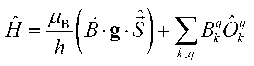 | (1) |
![[B with combining right harpoon above (vector)]](https://www.rsc.org/images/entities/i_char_0042_20d1.gif) for the static magnetic field, g for the g-tensor,
for the static magnetic field, g for the g-tensor,  for the total spin vector operator, Ôqk for spin operator equivalents for the corresponding spherical harmonics, and Bqk for the numeric coefficients for each of the spherical harmonics operators using the extended Stevens operator notation. In the EPR spectral simulations performed in this work, we assume an isotropic g-tensor that is described by a single g-value of g = 1.992. Due to time invariance, in the above sum only operators with even rank are allowed non-zero coefficients. For the total spin S = 7/2 of the Gd(III) ion, only operators of the rank 2, 4, and 6 are allowed.
In principle, all of the coefficients Bqk can be determined from EPR data. Such studies were reported for Gd(III)-doped single crystals, where the angular dependencies of EPR transitions could be precisely determined. It was found in these studies that the ZFS parameters were nearly identical among all detected Gd(III) centers within in each particular single crystal.9,25 In these cases, fitting a rather large number of ZFS coefficients from eqn (1) to angle-resolved EPR data produced a reliable output. However, in all reported cases of Gd(III) complexes in frozen glassy solutions, the EPR spectra reveal rather broad distributions of the ZFS parameters.1,2,26 In frozen glassy samples, where orientations are isotropically distributed and ZFS parameters broadly distributed, one does not have access to the detailed angle-resolved information provided by EPR spectra of a crystalline sample. Rather, all spin Hamiltonian parameters need to be determined from a single EPR spectrum or from a series of EPR spectra measured at different microwave frequencies. In this case, one cannot expect a stable fit if all of the higher-order operators in the spin Hamiltonian are included.23,26
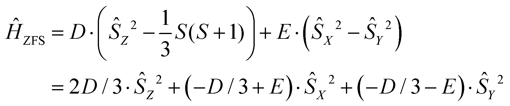
The modeling of EPR spectra for frozen glassy solutions of Gd(III) complexes is therefore performed under the simplification that only terms quadratic in total electron spin operators are left in the spin Hamiltonian. The commonly used form of the ZFS term in the spin Hamiltonian is given by
 | (2) |
If the eigenvalues of the ZFS tensor in its eigenframe are given as DX, DY and DZ, then the coefficients D and E in eqn (2) are defined as  and
and  . It follows that
| DX = −D/3 + E; DY = −D/3 − E; DZ = 2D/3. | (3) |
| |DX| ≤ |DY| ≤ |DZ| | (4) |
In order to determine the ZFS parameters of a particular Gd(III) complex one needs to fit two distributions, P(D) and P(E), to the measured EPR spectra. As a result of the above definitions, it is convenient to fit for the distribution P(E/D) instead of fitting for P(E) directly, since P(E/D) always assumes the same range of values 0 ≤ E/D ≤ 1/3 according to the above convention.
ZFS distributions in Gd(III) chelate complexes are rather broad. It is thus feasible to assume essentially uncorrelated distributions for the eigenvalues of the ZFS tensor. Correlations between D and E values would then only appear due to the above mentioned convention, and the distributions of D and E/D could be assumed to be uncorrelated. It is worth mentioning that similar EPR works were done for other S-state ions, like Fe(III) or Mn(II), and different variants of data analysis, including model free 1D and 2D fits, correlated or uncorrelated D, E, or E/D distributions, were tested.28–34 In this respect, however, one has to keep in mind that for iron and manganese the d orbitals are less compact as compared to the f orbitals of Gd(III). This leads to a stronger covalent character of the metal–ligand interactions in the d element complexes, which also affects strength, distribution widths and correlations of the ZFS parameters. The results of the cited publications, thus, have only restricted relevance to the study presented here.
For Gd(III) case, fitting many-parameter distributions for D and E (or E/D) is not practical, since such fit would be unstable and likely produce multiple solutions of comparable quality. Since the relatively featureless EPR spectra of Gd(III) complexes suggest broad ranges of ZFS parameters, simple models for the form of the distributions of D and E (or E/D) are often assumed to reduce the number of free parameters in the fit. This problem was tackled in two different ways in the reports of Raitsimring et al.23 and Benmelouka et al.24 The models for the ZFS parameter distributions proposed in these works are briefly summarized next. Their relation to the superposition model for realistic coordination geometries will be discussed in Section 5.
2.1 Model 1 (Benmelouka et al.)
The simplest model for the distributions of D and E in the ZFS term of the spin Hamiltonian (eqn (2)) was tested by Benmelouka et al.24 The authors assumed that the distributions of D and E for Gd(III) complexes in frozen glassy solutions can be described by two uncorrelated Gaussian distributions (drawn schematically in Fig. 1(a)), which we write here in the standard form: | (5) |
| Δ = |DZ| | (6) |
 | (7) |
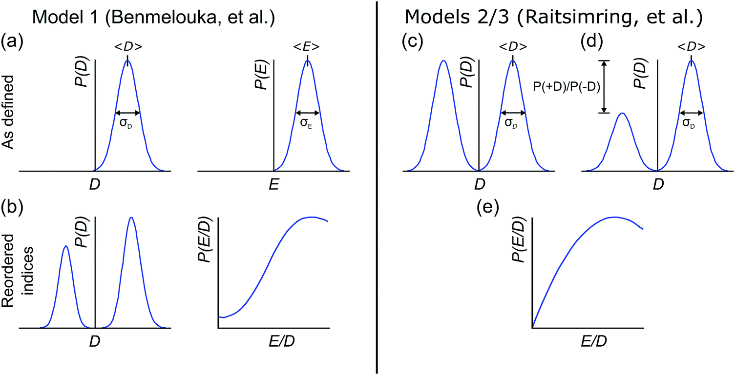 | ||
| Fig. 1 Graphical representation of the models used in this work for the distributions of the ZFS parameters D and E (or E/D). (a) Model 1 assumes that P(D) and P(E) are described by two uncorrelated Gaussian distributions. (b) Reshuffling of the indices to correct for the inconsistencies of Model 1 with the conventional definitions of the D and E parameters results in a bimodal Gaussian distribution. (c) Model 2 assumes P(D) is a bimodal Gaussian distribution, where the positive (D > 0) and negative (D < 0) contributions have equal amplitude and width. (d) Model 3 adds an asymmetry parameter (denoted P(+D)/P(−D)) to Model 2, which allows the relative amplitudes of the positive and negative contributions to the P(D) distribution to vary. (e) For Models 2 and 3, P(E/D) follows a polynomial distribution given by P(E/D) ∝ (E/D) − 2 × (E/D)2. | ||
Unlike P(D), the distribution of P(Δ) has a physically meaningful mean value and standard deviation. The axiality ξ is zero for E = 1/3, where the assignment of DY and DZ, and thus the sign of DZ is undefined, and has an absolute value of 1 for axial symmetry (E = 0). The axiality ξ is negative if DZ is negative and positive if DZ is positive ESI.† A provides a more detailed explanation of the characterization of the ZFS parameter distribution by the anisotropy Δ and axiality ξ parameters.
2.2 Models 2 and 3 (Raitsimring et al.)
Another approach to model the broad distributions of ZFS parameters D and E was suggested by Raitsimring et al.23,26 The ZFS parameter distributions were built under the approximation that the ZFS term can be represented as a linear combination of the ZFS contributions from the individual coordinating atoms of the ligand, where each of these donor atoms is assumed to be identical, and contribute an axial (E = 0) ZFS of magnitude D directed along the bond between the Gd(III) ion and the donor atom. This model was then incorporated into Monte Carlo simulations where the donor atoms were assumed to have randomly distributed positions on a spherical shell with the Gd(III) ion at its center. To exclude ligand clashes, any two ligand–metal bonds were restricted to form an angle of at least 60 degrees. This Monte Carlo modeling led to bimodal P(D) distributions, with the centers of the two approximately Gaussian modes of the distribution placed nearly symmetrically with respect to D = 0. This distribution was found to well describe EPR spectra for several Gd(III) complexes, even though they could not be physically described by a fully random distribution of ligands around the Gd(III) ion, due to the structures of the chelators. When applying this model to fit experimental EPR spectra, this distribution was simplified to a bimodal Gaussian distribution, in which the positive (D > 0) and negative (D < 0) modes of the P(D) distribution are assumed to have equal amplitude and width. The distributions P(E/D) were found to be slightly different for the positive and negative modes, but could be approximately described by a polynomial function of the form| P(E/D) ∝ (E/D) − 2·(E/D)2. | (8) |
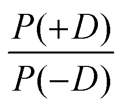
In order to discuss the effect of the bimodality of the distribution of the ZFS parameter D, we shall consider two versions of the ‘Raitsimring distribution’. In Model 2, we fix the relative weights of the positive and negative modes of the P(D) distribution to be equal. In Model 3, we allow different relative weights (amplitudes) for the positive (D > 0) and negative (D < 0) Gaussian modes of the P(D) distribution, denoted by P(+D)/P(−D). This asymmetry in the bimodal P(D) distribution was observed in the Monte Carlo simulations of Raitsimring et al.,23 and was found in the present work to be necessary to account for the experimentally observed asymmetry of the Gd(III) EPR spectra at high fields. The P(D) and P(E/D) distributions defined by Models 2 and 3 are sketched in Fig. 1(c)–(e).
3 Experimental and computational details
3.1 Synthesis of the Gd(III) complexes
The series of the six Gd(III) complexes 1–7 (Fig. 2) was chosen to be included in this work. Gd-DOTA (2) was obtained commercially from macrocyclics and used without further purification. The synthesis details of the complexes Gd-NO3Pic (1), Gd-maleimide-DOTA (3), iodo-(Gd-PyMTA) (4a), MOMethynyl-(Gd-PyMTA) (4b), Gd-TAHA (5), iodo-(Gd-PCTA-[12]) (6), and Gd-PyDTTA (7) are given in the ESI.† | ||
| Fig. 2 Structural formulae and naming of the Gd(III) complexes 1–7 which were studied in this work. Please note that in the case of Gd-TAHA (5) and Gd-PyDTTA (7) no crystal structures are available, and the dotted lines only indicate possible ligand atom-Gd(III) ion interaction. | ||
For the complexes iodo-(Gd-PyMTA) (4a) and MOMethynyl-(Gd-PyMTA) (4b), we assume that the substituents iodo and MOMethynyl do not have a strong influence on the ZFS parameter distributions. This assumption is supported by nearly identical Q-band (34 GHz) spectra (see ESI,† Fig. B.1).
3.2 Sample preparation
For Q- and W-band measurements, stock solutions of the Gd(III) complexes were diluted to a final concentration of 25 μM in 1![[thin space (1/6-em)]](https://www.rsc.org/images/entities/char_2009.gif) :1 (v:v) D2O/glycerol-d8. Sample solutions were filled into 3 mm o.d. quartz capillaries for Q-band measurements and 0.5 mm i.d./0.9 mm o.d. quartz capillaries for W-band measurements and subsequently flash frozen in liquid nitrogen under ambient conditions. For 240 GHz measurements, stock solutions of the Gd(III) complexes were diluted to a final concentration of 300 μM in 0.4:0.6 (v:v) D2O/glycerol-d8. Sample solutions of 10 μL volume were loaded into a Teflon sample cup of ∼3.5 mm i.d. and ∼5 mm height and subsequently flash frozen in liquid nitrogen under ambient conditions.
:1 (v:v) D2O/glycerol-d8. Sample solutions were filled into 3 mm o.d. quartz capillaries for Q-band measurements and 0.5 mm i.d./0.9 mm o.d. quartz capillaries for W-band measurements and subsequently flash frozen in liquid nitrogen under ambient conditions. For 240 GHz measurements, stock solutions of the Gd(III) complexes were diluted to a final concentration of 300 μM in 0.4:0.6 (v:v) D2O/glycerol-d8. Sample solutions of 10 μL volume were loaded into a Teflon sample cup of ∼3.5 mm i.d. and ∼5 mm height and subsequently flash frozen in liquid nitrogen under ambient conditions.
3.3 Q-, W- and G-band EPR measurements
Q-band (∼34 GHz) measurements were performed on a home-built high-power Q-band pulse EPR spectrometer36 equipped with a rectangular cavity accommodating oversized 3 mm outer diameter cylindrical samples.37,38 W-band (∼94 GHz) spectra were recorded on a Bruker Elexsys E680 X-/W-band spectrometer using a EN 680-1021H resonator. The measurement temperature was stabilized by a Helium-flow cryostat (ER 4118 CF, Oxford Instruments) to 10 K. Echo-detected (ED) field-swept EPR spectra were acquired using the Hahn-echo pulse sequence tp − τ − 2tp − τ with a pulse length tp of 12 ns. The interpulse delay τ was set to 400 ns. The power to obtain π/2–π pulses of 12–24 ns was determined at the central transition of the Gd(III) spectrum by nutation experiments. Resulting Q-/W-band spectra had a constant field and baseline offset removed and were normalized to the maximum for comparison with the simulated spectra.G-band (240 GHz) EPR measurements were carried out on a home-built spectrometer, as described elsewhere.39,40 A solid-state frequency-multiplied source (Virginia Diodes, Inc.) with CW power of ∼50 mW at 240 GHz was used. Incident microwave power was adjusted as needed by voltage-controlled attenuation of the source and a pair of crossed wiregrid polarizers. The spectrometer operates in induction mode detection with a quasi-optical bridge, superheterodyne detection with a Schottky subharmonic mixer (Virginia Diodes, Inc.), and a home-built intermediate frequency (IF) stage operating at 10 GHz. The IF signal is mixed down to baseband for detection in quadrature with a pair of lock-in amplifiers (Stanford Research Instruments, Inc. SR830).
The Teflon sample cup was backed by a mirror and mounted within a modulation coil at the end of an overmoded waveguide (Thomas Keating Ltd). No resonant cavity was used. This assembly was then loaded into a continuous flow cryostat (Janis Research Company) mounted in the room-temperature bore of the magnet. Measurements were carried out at a sample temperature of approximately 5 K. Sample temperature was monitored with a Cernox temperature sensor (Lakeshore Cryogenics Inc.), mounted at the end of the waveguide near the sample position. Recorded sample temperatures for each measurement are given in Table G.5 (ESI†). EPR spectra at 240 GHz were acquired using a rapid passage technique, which is similar in practice to CW EPR but records an absorption lineshape rather than a derivative lineshape.24,41,42 Rapid passage EPR measurements were carried out with field modulation at 20 kHz with ∼0.3 mT modulation amplitude. The main coil of the superconducting magnet (Oxford Instruments), which is sweepable from 0–12.5 T, was used to carry out measurements at a sweep rate of 0.1 T min−1. Initial calibration experiments with Gd(III) complexes indicated that, given the range of experimental parameters available in this 240 GHz EPR spectrometer, the rapid passage regime could be entered by simply increasing the microwave power when the sample is held at 5 K. Once the microwave power was sufficiently high to achieve a passage regime, a further increase of the applied microwave power resulted only in a change in the SNR of the signal and the saturation of the central |−1/2〉 ↔ |+1/2〉 transition. Changing the sweep rate of the magnetic field or the modulation frequency and amplitude was found to not affect the transition from the CW to the rapid passage regime for the range of values tested, and therefore these experimental parameters were set so as to optimize SNR. Linearity of the magnetic field over the sweep range was verified with independent measurements using a Mn:MgO field standard.43,44 The measured 240 GHz spectra has a constant baseline removed and were normalized to the envelope resulting from the outer EPR transitions for comparison with simulated spectra, as the relatively high powers and fast sweep rate necessary to collect data in the rapid passage regime were found to artificially broaden the very narrow central transition of Gd(III).
3.4 Numerical simulations
The EPR spectra of Gd(III) complexes were simulated in MATLAB (The MathWorks Inc., Natick, MA, USA) with home written scripts based on the EasySpin toolbox.45 Absorption powder spectra were computed using full matrix diagonalization with the EasySpin function pepper. The spin system structure in EasySpin was defined as a single spin S = 7/2 with an isotropic g-value of 1.992. The strains for g, D, and E were set to zero in the EasySpin spin system structure. This was done because in the EasySpin package the EPR line broadening resulting from a strain on these parameters is computed using a linear approximation. This linear approximation is sufficiently accurate for small strains, but becomes imprecise for large ones where the strain is comparable to the mean values of D and E values. Therefore, all calculations in this work were performed by generating the distributions P(D) and P(E) (or P(E/D)) according to one of the three models described in the previous section, computing an EPR spectrum for each pair (D,E) with the EasySpin function pepper, and summing these spectra with the weights W(D,E) according to the probability products: W(D,E) = P(D)·P(E). Unless otherwise noted, additional line broadening parameters were set to zero in the simulations.Orientation averaging was performed in 3 degree increments and a 10-fold interpolation of the orientation grid. The magnetic field range for simulation was chosen to well cover the experimental one, as the EasySpin function pepper forces the computed spectra to zero at its boundaries. The number of field points was set to 8000 to reach sufficient convergence. The simulation output was set to separate the subspectra computed for each transition of the S = 7/2 spin system. For the 240 GHz spectra, whose data were obtained by rapid passage measurements, the contributions of the individual transitions were summed as is to arrive at the final simulated spectra. For the spectra obtained from echo-detected field-swept EPR measurements (Q/W band), the contributions of the individual transitions were summed with a weighting factor according to their effective flip angles (SI C.5, ESI†).
Two different approaches to the sampling of the P(D) and P(E) (P(E/D)) distributions were investigated. First, the distributions of ZFS parameters were sampled using a regular grid of points. Second, a Monte-Carlo approach was used in which a large set of randomly distributed (D,E) pairs was generated and the overall EPR spectrum is computed as a linear combination of the EPR spectra for all of those pairs. It was found in the course of this work that the Monte-Carlo sampling of the P(D) and P(E) (or P(E/D)) distributions resulted in the optimal computation cost and avoided unphysical artifacts in the simulated spectra associated with oversampling in the vicinity of the D = 0 point of the P(D) distribution. Note that both approaches require careful calibration of the number of random steps in the Monte Carlo scheme, or equivalently, of the step size in the regular grid, in order to reach convergence of the simulated EPR spectrum.
Extensive details of the numerical simulations, including convergence tests, can be found in SI C (ESI†). For all simulations presented in the main body of the paper, the Monte-Carlo approach to sampling of the P(D) and P(E) (or P(E/D)) distributions was used.
4 Results and analysis
The simulated EPR powder spectra of Gd(III) complexes predominantly consist of seven allowed transitions |mS〉 ↔ |mS + 1〉, broadened by the anisotropy of the ZFS interaction. According to Kramers' theorem, for a half-integer spin the levels |±mS〉 are degenerate in zero magnetic field. For weak ZFS (as compared to the EZ interaction) the subspectrum of the central |−1/2〉 ↔ |+1/2〉 transition is much narrower than the other transitions of the Gd(III) complex, which primarily contribute to the broad envelope of the total lineshape.46 This spectral feature results from the |−1/2〉 ↔ |+1/2〉 transition being broadened by ZFS to second (and higher) order of the perturbation series on the hD/gμBB parameter, while the other Gd(III) transitions are broadened to first order by ZFS. Due to this scaling of the width of the |−1/2〉 ↔ |+1/2〉 transition with the magnetic field strength, the relative width of this transition with respect to the full width of the Gd(III) EPR spectrum decreases with increasing detection field/frequency.An illustration of this spectral feature is given in Fig. 3. Note also that at high fields and low temperatures the relative integral intensities of the different Gd(III) subspectra are not equal. At 10 K, the narrow central transition dominates the spectra in Q band (∼34 GHz) and W band (∼94 GHz). The increasing relative contribution of the EZ interaction as compared to ZFS in W band leads to a narrowing and higher relative peak amplitude of the central transition as compared to Q band. A predominant population of the lowest energy levels at 5 K and 240 GHz induces a change in the relative intensities of the different sublevels resulting in the broad envelope of the |−7/2〉 ↔ |−5/2〉 transition subspectrum dominating the Gd(III) spectral shape. The line shape of this outer transition is most asymmetric with respect to the position of the narrow peak of the central transition with a shift towards lower fields for positive D distributions and towards higher fields for negative D distributions. If both positive and negative modes are present in the P(D) distribution, the remaining anisotropy of the EPR line shape indicates a difference in the weights of these two modes (e.g. in Model 3).
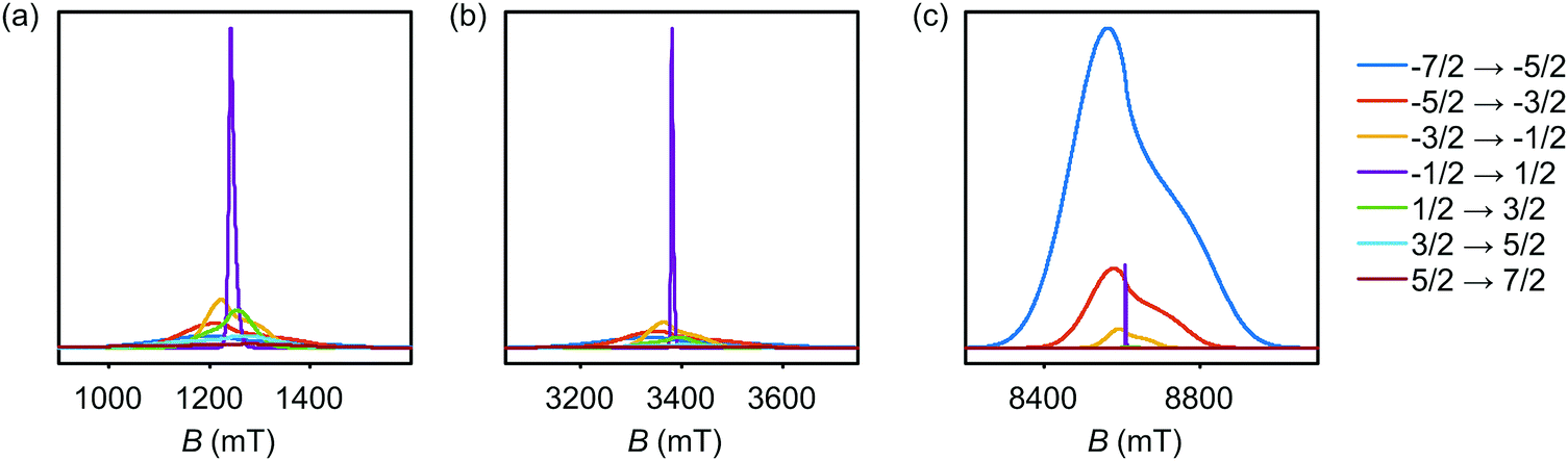 | ||
| Fig. 3 Evolution of allowed EPR transitions as a function of field/frequency and temperature for an unimodal P(D) distribution with 〈D〉 = 1200 MHz, σD = 400 MHz, and P(E/D) as given in eqn (5). (a) Q band and 10 K, (b) W band and 10 K, (c) G band and 5 K. | ||
4.1 Model 1
The multi-frequency set of EPR spectra for the six Gd(III) complexes were simulated with Model 1 using visual inspection to obtain an estimate of the parameter space, and so to evaluate the performance of the model. In these initial simulations for Model 1, the variables D, σD, E, σE, and a small convolutional line broadening term (Sys.lwpp in EasySpin) were taken as free parameters. The visually optimized EPR simulations for the complexes Gd-NO3Pic (1) and Gd-PyDTTA (7) are shown in Fig. 5. The analogous simulations for all other complexes are found in SI H (ESI†).In the analysis using Model 1, it was found that in certain cases a conflict can arise in the definitions of the distributions P(D) and P(E) as a pair of uncorrelated Gaussian distributions (eqn (5)). It has been found in our results and in those reported by other authors23,24,47 that the widths (σD and σE) of the P(D) and P(E) distributions are typically smaller, but comparable to the average values 〈D〉 and 〈E〉. In this situation, two uncorrelated Gaussian distributions for P(D) and P(E) produce a large fraction of cases where either D and E have different signs, or where the signs of D and E are the same but the relation |E| ≤ |D/3| does not hold. In such cases, one can still formally write eqn (2) for any pair of values D and E and compute the values DX, DY, and DZ according to eqn (3). However, in order to satisfy the conditions of eqn (4), one would have to reshuffle the indices (X,Y,Z) of the computed DX, DY and DZ values. After such an index rearrangement, the D and E values need to be newly computed. The resulting distributions of P(D) and P(E/D) after this index rearrangement are sketched in Fig. 1(b). An example calculation carrying out this reordering of the P(D) and P(E) distributions is shown for Gd-NO3Pic (1) and Gd-PyDTTA (7) in Fig. 4, with the corresponding ZFS parameters given in Table 1. The corrected P(D) and P(E) distributions are both bimodal with different weights of the positive and negative components. The distribution of P(E/D) fully covers the allowed range from 0 to 1/3, with a significant probability density at E/D = 0 for some of the Gd(III) complexes (e.g. for Gd-NO3Pic (1) in Fig. 4). The maximum of the probability distribution P(E/D) appears in the vicinity of the value 〈E〉/〈D〉. Overlaying the newly obtained D distribution by two Gaussians shows that the maxima are slightly asymmetric with respect to zero and shift towards larger values for the dominant component. Additionally, the widths of the two new Gaussian distributions are reduced compared to the width of the input distribution.
 | ||
| Fig. 4 Distribution of ZFS parameters for Model 1 as defined in eqn (5) (black) and after rearranging of the indexes (X,Y,Z) of the computed DX, DY and DZ values (light blue) for the Gd(III) complexes Gd-NO3Pic (1) and Gd-PyDTTA (7). Gaussian distributions are overlaid over the rearranged P(D) distributions (red dashed lines). Distributions are scaled so that the area under the curves integrates to 1. (a and d) P(D) distributions, (b and e) P(E) distributions, and (c and f) P(E/D) distributions. The green line shows P(E/D) defined in eqn (8),23 used in the simulations with Models 2 and 3 in this manuscript. | ||
 | ||
| Fig. 5 EPR spectra (black lines) and corresponding fits (light blue lines) obtained using Model 1 and the ZFS parameters given in Table 2 for the complexes Gd-NO3Pic (1) and Gd-PyDTTA (7). Q band spectra at 10 K, W band spectra at 10 K, and G band spectra at approximately 5 K. | ||
| Complex | D init | D pos | D neg | σ D,init | σ D,pos | σ D,neg |
|
|---|---|---|---|---|---|---|---|
| Gd-NO3Pic (1) | 420 | 472 | −418 | 140 | 124 | 111 | 1.4 |
| Gd-PyDTTA (7) | 1800 | 1845 | −1275 | 514 | 439 | 271 | 3.3 |

Table 2 summarizes the ZFS parameter values for Model 1 determined by visual inspection before reordering of the indices. The values obtained after reordering of the indices are given for Gd-NO3Pic (1) and Gd-PyDTTA (7) in Table 1, and for the remaining Gd(III) complexes in Table S4.2 of the ESI.† For Model 1, we find that the width σD lies between 29–40% of 〈D〉 and that 〈E〉 corresponds to approximately 25% of the value of 〈D〉 (Table 2). The width σE is 33–50% with respect to 〈E〉, which corresponds to the main fraction of the P(E/D) distribution used in Models 2 and 3. For the Gd(III) complexes Gd-NO3Pic (1), R-(Gd-PyMTA) (4ab), and Gd-TAHA (5), showing rather symmetric EPR spectra, the ratio of E/D is higher than for the complexes Gd-PyDTTA (7) and iodo-(Gd-PCTA-[12]) (6), which exhibit more asymmetric EPR spectra. Thus, for complexes with rather symmetric EPR spectra a shift of the maximum of the P(E/D) distribution towards E/D = 1/3 is observed, while the maxima of the P(E/D) distribution of asymmetric EPR spectra are shifted towards smaller values (see Fig. 4(c) and (f)). This observation was discussed previously by Raitsimring et al.23
 and mean ZFS axiality
 ![[small xi, Greek, macron]](https://www.rsc.org/images/entities/i_char_e0cf.gif) can be found in the ESI Table P.9
can be found in the ESI Table P.9
| Model | Complex | D (MHz) | σ D (MHz) |
|
|
E (MHz) | σ E (MHz) |
|
|
lwpp (mT) |
|---|---|---|---|---|---|---|---|---|---|---|
| 1 | Gd-NO3Pic (1) | 420 | 140 | 0.33 | — | 120 | 60 | 0.50 | 0.29 | [0.5 0] |
| Gd-DOTA (2)/Gd-maleimide-DOTA (3) | −600 | 240 | 0.40 | — | 150 | 75 | 0.50 | 0.25 | [1.0 0.1] | |
| R-(Gd-PyMTA) (4a,b) | 1070 | 357 | 0.33 | — | 306 | 153 | 0.50 | 0.29 | [0.8 0] | |
| Gd-TAHA (5) | 1250 | 417 | 0.33 | — | 357 | 119 | 0.33 | 0.29 | [0.6 0] | |
| Iodo-(Gd-PCTA-[12]) (6) | 1780 | 508 | 0.29 | — | 396 | 132 | 0.33 | 0.22 | [1.0 0.1] | |
| Gd-PyDTTA (7) | 1800 | 514 | 0.29 | — | 400 | 133 | 0.33 | 0.22 | [2.0 0.1] | |
| 2 | Gd-NO3Pic (1) | 500 ± 19 | 169 ± 52 | 0.34 | — | — | — | — | — | [0 0] |
| Gd-DOTA (2)/Gd-maleimide-DOTA (3) | 652 ± 44 | 409 ± 200 | 0.63 | — | — | — | — | — | [0 0] | |
| R-(Gd-PyMTA) (4a,b) | 1263 ± 112 | 350 ± 109 | 0.28 | — | — | — | — | — | [0 0] | |
| Gd-TAHA (5) | 1335 ± 75 | 408 ± 178 | 0.31 | — | — | — | — | — | [0 0] | |
| Iodo-(Gd-PCTA-[12]) (6) | 1845 ± 194 | 400 ± 289 | 0.22 | — | — | — | — | — | [0 0] | |
| Gd-PyDTTA (7) | 1810 ± 173 | 367 ± 289 | 0.20 | — | — | — | — | — | [0 0] | |
| 3 | Gd-NO3Pic (1) | 485 ± 20 | 155 ± 37 | 0.32 | 1.8 | — | — | — | — | [0 0] |
| Gd-DOTA (2)/Gd-maleimide-DOTA (3) | 714 ± 43 | 328 ± 99 | 0.46 | 0.3 | — | — | — | — | [0 0] | |
| R-(Gd-PyMTA) (4a,b) | 1213 ± 60 | 418 ± 141 | 0.34 | 1.6 | — | — | — | — | [0 0] | |
| Gd-TAHA (5) | 1361 ± 69 | 457 ± 178 | 0.34 | 1.9 | — | — | — | — | [0 0] | |
| Iodo-(Gd-PCTA-[12]) (6) | 1861 ± 135 | 467 ± 292 | 0.25 | 3.6 | — | — | — | — | [0 0] | |
| Gd-PyDTTA (7) | 1830 ± 105 | 390 ± 242 | 0.21 | 3.6 | — | — | — | — | [0 0] | |


Comparing the corrected P(D) and P(E/D) distributions for Models 1 and 3 (see ESI,† Fig. O.25), we can make a few important notes. First, the corrected P(D) distributions found for Model 1 can be rather closely approximated by the asymmetric bimodal P(D) distribution of Model 3. Note that the widths of the two modes of the corrected P(D) distribution for Model 1 are somewhat smaller than the initial width of the non-corrected single Gaussian distribution. This is important to keep in mind when comparing literature data for ZFS parameter values obtained with Model 1 to the analogous ZFS parameter values obtained with Model 3. Second, the corrected P(E/D) distribution has a minimum probability density at E/D = 0 and a maximum probability density around 〈E〉/〈D〉 = 0.25, which is again similar to the P(E/D) distribution in Model 3. However, the overall similarity of the P(E/D) distributions for Models 1 and 3 is not as good as for the P(D) distributions. The maximum of the P(E/D) distribution of Model 1 is not at exactly 〈E〉/〈D〉 = 0.25 but rather deviates from this value by about 15% for the various Gd(III) complexes. Additionally, the probability density at E/D = 0 is zero in Model 3, but usually assumes a nonzero value in Model 1.
Models 1 and 3, while differently defined, both appeal to physical intuition. Model 1 appeals to the central limit theorem, which, however, requires the presence of a virtually unlimited number of different randomly distributed donor atom contributions to the P(D) and P(E) distributions in order to be strictly valid. Model 3 appeals to the near equality of ZFS contributions for all ligands and to the non-directional character of the bonds in the Gd(III) complex. Model 3 also includes flexibility to vary the relative weights of the positive and negative modes in the P(D) distribution, while for Model 1 with a given set of D, E, σD, and σE, the relative weights of the positive and negative mode of the P(D) distribution are fixed. After recognizing that Models 1 and 3 result in rather similar distributions of ZFS parameter values, with some additional flexibility available in Model 3, we turn to a more detailed analysis of the Gd(III) ZFS parameter distributions using Models 2 and 3.
4.2 Models 2 and 3
Model 3 was initially investigated by visual inspection to determine ZFS distribution parameters for each of the Gd(III) complexes. The results of this visual comparison of the experimental data with simulated EPR spectra for different (D, σD) pairs and P(+D)/P(−D) ratios are given in SI K (ESI†). It was observed that for rather broad ranges of the ZFS distribution parameters the correspondence between experimental and simulated data was quite good. In such a case, reporting a single best-fit set of values does not capture this range of possible variations of the ZFS distribution parameters. In order to assign error bars to the determined ZFS parameter values, we monitored the RMSD between the experimentally determined and the simulated lineshapes over a wide range of ZFS parameter values as follows.To formalize the determination of error bars on the determined ZFS parameters for Models 2 and 3, we generated a large library of simulated spectra for each measurement frequency and temperature. This library maps out a region of the parameter space spanning values of D = 300–1950 MHz and σD = 50–600 MHz in steps of 50 MHz, chosen so as to include the expected values of these parameters for the Gd(III) complexes studied here, as estimated from our initial investigations by visual inspection. In order to have a common library to query all Gd(III) complexes studied in this work, typical values for the measurement frequency (in Q and W band) and temperature (in G band) were used in place of the exact experimental values for each Gd(III) complex, as detailed in the ESI† (Table E.2). The small measurement to measurement deviations in frequency and temperature from these typical values were found to not significantly impact the line shape of the simulated EPR spectra, and hence are not expected to alter the final determined ZFS parameter values. For this library of simulations, the contributions to the line shape from each transition and from the positive and negative modes of the P(D) distribution according to Models 2 and 3 were saved separately. In this way, the same library may be used for both Models 2 and 3, by either summing these contributions as is, or by adding a weighting term denoted P(+D)/P(−D) which introduces an asymmetry in the P(D) distribution for Model 3. Further details of the inputs used to generate the library of simulated spectra can be found in SI E (ESI†).
Each lineshape in the library of simulated spectra was compared to the data at the corresponding frequency by scaling the amplitude of the simulation to best fit the baseline-corrected experimental data in a least-squares sense. The RMSD between each simulation and the experimentally obtained data was then computed according to
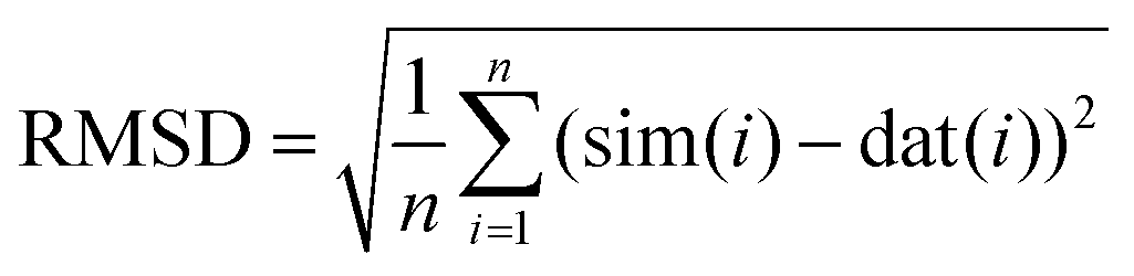 | (9) |
For all three models, the contribution from complexes with very small ZFS (corresponding to the region of the P(D) distribution near D = 0) is still sufficiently large to produce a sharp feature in the vicinity of the Gd(III) g-value position in the simulated EPR spectra. This results in the models predicting a sharper feature than is experimentally observed in the field range spanning the middle of the central peak of the Gd(III) EPR spectrum (see SI C.4, ESI†). It is rather difficult to define precisely the field range where this distortion of the shape of the central peak is significant, since no clear ‘kinks’ are observed between the middle and the outer parts of the central transition. This overly sharp feature in the simulated spectra can be smeared out by introducing an intrinsic linewidth as a ‘beautifying parameter’ (see SI C.4, ESI†). However, in the RMSD analysis with Models 2 and 3 we attempted to avoid introducing additional free parameters into the fit. As an alternative and straightforward approach, we completely excluded the region of the central transition of the EPR spectra from the fit. The parts of the spectra in the remaining field ranges to the left and to the right of the central peak region were then used to compute the RMSD error.
The dependence of the RMSD on the D and σD values input in the simulation can be visualized as RMSD error maps (e.g. shown for Model 2 and the Gd(III) complexes Gd-NO3Pic (1) and Gd-PyDTTA (7) in Fig. 6), where the lines represent contours of constant RMSD and the asterisk denotes the value of D and σD with the minimum RMSD value on the 50 MHz grid of ZFS parameter values at the given EPR frequency. Each plotted contour line represents a doubling of the minimum RMSD value. RMSD error maps for all of the Gd(III) complexes fitted with Model 2 with the region about the central peak excluded are given in the ESI† (Fig. I.10).
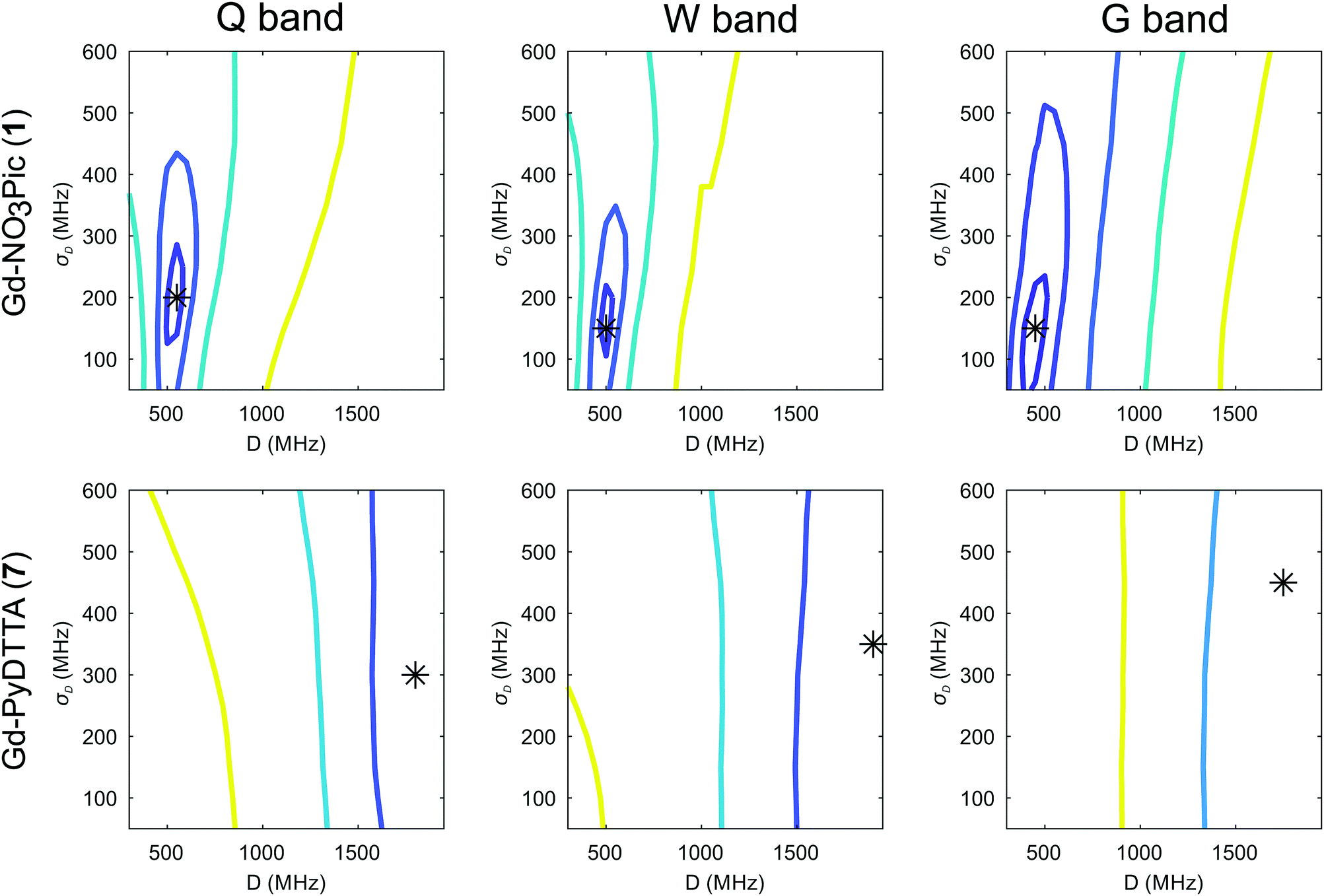 | ||
| Fig. 6 Contours of constant RMSD as a function of D and σD parameter values using Model 2 for the complexes Gd-NO3Pic (1) and Gd-PyDTTA (7) in Q band and 10 K, W band and 10 K, and G band and 5 K. Simulated spectra were normalized to the experimental data using only the outer shoulders of the spectra. The asterisk denotes the set of parameter values available in the library of simulated spectra which has the minimum RMSD value for each measurement frequency. Each contour line represents a doubling of this minimum RMSD value. | ||
It should be noted that in this work and in studies reported in the literature,23,24 one attempts to describe the ZFS interactions in an ensemble of Gd(III) complexes using a simplified model for the ZFS parameter distributions. While these simplified models seem to be reasonably accurate, as evidenced by the rather good fits to the experimental data, this does not necessarily mean that the given model accurately describes the physical system. Such an inadequacy is implied in the deviation of the best fit simulations exceeding the noise level of the experimental data. This means that the minimum RMSD between experimental and simulated EPR spectra will not approach zero even for EPR spectra with extremely high signal-to-noise ratio (SNR). Additionally, the D and σD values corresponding to the minimum RMSD value in the contour plots are not exactly identical for the three tested microwave bands, again indicating the approximate nature of these models. Therefore, while it is possible to characterize the precision of the determined ZFS parameter values within a model, it is not possible to ascertain the physical accuracy of these values in an absolute sense.
To obtain a conservative estimate for the precision of the determined ZFS parameter values, we look for the variations of ZFS parameters around the best fit values and take as an acceptable fit those values which result in an RMSD less than twice the minimum RMSD value. If the problem was linear and the RMSD dominated by noise, this choice would correspond to a 95% confidence interval. The first contour line about the minimum RMSD value gives the region where the RMSD doubles, as shown in e.g.Fig. 6, and this is consistently done for all other contour plots in this work. However, the 50 MHz grid of ZFS parameters available in the library of simulated EPR spectra is a somewhat coarse sampling of these parameter values, particularly for complexes with small ZFS. In order to interpolate the ZFS parameter values on this grid, we make the assumption that the contour bounding the region of twice the minimum RMSD value should be smooth given arbitrarily fine sampling of D and σD values. Therefore, we estimate this contour by fitting an ellipse, from which the best fit values of D and σD is taken to be given by the center of an ellipse fit to this first contour line. The errors on the D and σD parameters are given by the lengths of the semi-minor and semi-major axes of the fitted ellipse. Taking a weighted average of the so-determined values for D and σD and their associated errors at each frequency (SI F, ESI†) gives our final results with Model 2, as summarized in Table 2.
The contour plots show that the value of D is rather well constrained for Model 2, and thus its actual physical value most likely does not deviate from the best-fit value for Model 2 by more than 10%. By comparison, the σD value is less well constrained in the fits with Model 2. In particular, for iodo-(Gd-PCTA-[12]) (6) and Gd-PyDTTA (7), the contour plots suggest that the σD value can assume essentially any allowed value. For the Gd(III) complexes with weaker ZFS, Gd-NO3Pic (1) and Gd-DOTA (2)/Gd-maleimide-DOTA (3), the σD value is somewhat better constrained by the fit. But even in the best case of Gd-NO3Pic (1) in W band, the σD value varies by ±30% within the area encompassed by the contour curve bounding the region of twice the minimum RMSD (Fig. I.10, ESI†).
Two examples of the EPR spectra simulated at the three microwave bands using the determined best-fit ZFS parameters for Model 2 (Table 2) are shown in Fig. 7 for the complexes Gd-NO3Pic (1) and Gd-PyDTTA (7). Full results for all the other Gd(III) complexes can be found in the ESI† (SI I). For EPR spectra in Q band and W band, Model 2 gives quite reasonable fits of the experimental data, despite the fixed equal ratio between the positive and negative modes of the P(D) distribution. Note that the position and width of the central peak is rather well reproduced by the simulation in Q band and W band, even though the region of this peak was excluded from the fit. However, the spectra measured in G band show strong deviations between the experimental data and their respective fits with Model 2.
 | ||
| Fig. 7 Simulations using the best-fit ZFS parameters for Model 2, with and without the region of the central transition included in the RMSD error map analyses, for the complexes Gd-NO3Pic (1) and Gd-PyDTTA (7). | ||
Model 3 is similar to Model 2, but with an additional allowance for the optimization of the relative contributions from the positive and negative modes of the P(D) distribution. The asymmetry of such a distribution can be defined by the ratio between the two amplitudes of the positive and negative modes of the P(D) distribution, which we denote P(+D)/P(−D). Note that P(+D)/P(−D) < 1 in Model 3 corresponds to D < 0 in Model 1 (case of Gd-DOTA, see Table 2), whereas P(+D)/P(−D) > 1 in Model 3 corresponds to D > 0 in Model 1 (all other complexes). The asymmetry P(+D)/P(−D) was determined by fixing the mean of D to the closest available value in the library of simulations to that determined using Model 2 (Table 2) and then varying P(+D)/P(−D) to find the best fit to the G-band data where the asymmetry in the EPR spectra is most prominent. We additionally attempted to determine P(+D)/P(−D) using the Q-/W-band data, but these spectra were not sufficiently sensitive to variations in this parameter to assign a best-fit value. It is interesting to visualize the effect of this parameter with RMSD contour plots of varying P(+D)/P(−D) and σD values, e.g. for Gd-NO3Pic (1) and Gd-PyDTTA (7) in Fig. 8. Contour plots are given for all of the Gd(III) complexes in the ESI† (Fig. J.13). In the following calculations with Model 3, we use the optimal P(+D)/P(−D) values as determined by the σD and P(+D)/P(−D) contour plots for consistency. Once the asymmetry parameter P(+D)/P(−D) was determined via the minimum RMSD value in this error map, that value was fixed and the (D, σD) RMSD error maps were recomputed for the three microwave bands to find the best-fit values of these parameters.
 | ||
| Fig. 8 Contours of constant RMSD as a function of P(+D)/P(−D) and σD parameter values using Model 3 and the complexes Gd-NO3Pic (1) and Gd-PyDTTA (7) in G band and 5 K. The mean values of the ZFS parameter D were set to D = 500 MHz and D = 1800 MHz, respectively, corresponding to the closet D value available in the library of simulations to the D value as determined by Model 2 for these complexes (Table 2). The asterisk denotes the position of minimum RMSD. | ||
It appeared that an error estimate by the parameter range bounded by a contour of twice the minimum RMSD may not be reasonable for the asymmetry parameter P(+D)/P(−D) in Model 3. The most obvious effect of this parameter on the EPR spectra is to set the relative position of the broad component of the spectrum with respect to the sharp central peak corresponding to the |−1/2〉 → |1/2〉 transition. This is because the width of this central peak is so narrow compared to the broad component of the 240 GHz EPR spectrum that it has a relatively small impact on the overall RMSD of the fit, though there is enough effect on the RMSD to assign a position of minimum RMSD in a contour plot of P(+D)/P(−D) and σD (e.g. in Fig. 8), as was done to determine the other parameter values for Models 2 and 3. It was found that the separation between the sharp central transition and the peak of the broad component of the 240 GHz EPR spectra varies approximately linearly with the determined P(+D)/P(−D) values. This was used to estimate a typical deviation of 0.34 for the value of the P(+D)/P(−D) parameter (8), though this varied for the different Gd(III) complexes. Practically, it was found to be difficult given the available data and models to assign an accurate ratio for the relative contributions of these two components of the P(D) distribution.
The final best-fit ZFS values from Model 3 with the region about the central peak excluded from the analysis are presented in Table 2, and the corresponding simulated spectra presented with the full dataset in Fig. 9 and 10. Including an asymmetry in the P(D) distribution helped to slightly better constrain the range for the σD values, but did not significantly alter the best-fit for the D and σD values (Fig. 11). For the Q-band and W-band spectra, the minimum RMSD of the (D, σD) contour plots was not significantly altered by the addition of the asymmetry parameter. For the G-band data, which displays the greatest degree of asymmetry in the measured spectra, the minimal RMSD value in the contour plots decreased by more than a factor of two in some cases with the addition of the P(+D)/P(−D) parameter in Model 3 compared to the fits using Model 2 (see ESI,† Fig. M.22).
 | ||
| Fig. 9 Measured EPR spectra in Q band, W band, and G band for the Gd(III) complexes Gd-NO3Pic (1), Gd-DOTA (2) (G-band spectra)/Gd-maleimide-DOTA (3) (Q-/W-band spectra), and iodo-(Gd-PyMTA) (4a) (G-band spectra)/MOMethynyl-(Gd-PyMTA) (4b) (Q-/W-band spectra). Overlaid are simulations with Model 3 using the best-fit ZFS parameters presented in Table 2. The faded regions indicate the portion of the spectra about the central transition which was excluded from the RMSD error map calculations. | ||
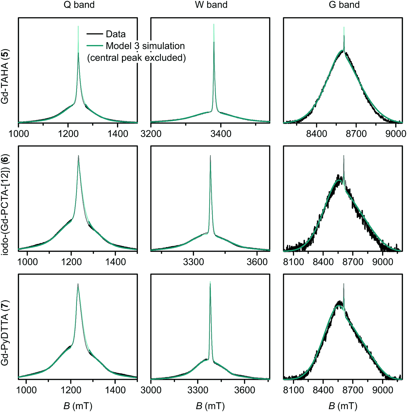 | ||
| Fig. 10 Measured EPR spectra in Q band, W band, and G band for the Gd(III) complexes Gd-TAHA (5), iodo-(Gd-PCTA-[12]) (6), and Gd-PyDTTA (7). Overlaid are simulations with Model 3 using the best-fit ZFS parameters presented in Table 2. The faded regions indicate the portion of the spectra about the central transition which was excluded from the RMSD error map calculations. | ||
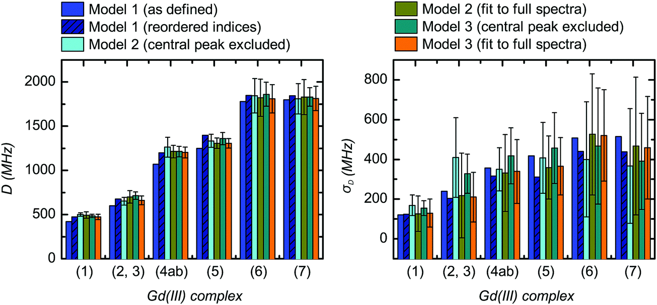 | ||
| Fig. 11 Comparison of the extracted values for the mean (〈D〉) and width (σD) of the ZFS parameter D for the three models and each of the tested Gd(III) complexes. Structural formulae and naming for the Gd(III) complexes 1–7 are given in Fig. 2. Model 1 was fit by visual inspection, and therefore error bars on the ZFS parameters D and σD were not computed. For Models 2 and 3, mean values and error bars for D and σD were computed by combining results from RMSD error maps which compare a library of simulated spectra to the data at the three measurement frequencies. Models 2 and 3 were fit with the region about the central transition excluded from analysis, and also with the full EPR spectra included in the analysis. | ||
We next investigated what changes would be induced by including the region of the central peak into the RMSD error map calculations. The RMSD contour plots, best-fit ZFS parameter values, and the corresponding best-fit spectra for Models 2 and 3 when including the full EPR spectra in the analysis are given in SI L (ESI†). In general, the deviations in the line shape in the region of the central peak lead to larger overall RMSD values as a result of the larger intensities in the portion of the spectra (Fig. M.22, ESI†). When the region of the central peak is included in the fit it dominates the RMSD for complexes with small ZFS. Even for complexes with large ZFS, the central transition still strongly affects the fit despite being broadened and thus displaying lower relative peak intensity. We additionally find that the range of D values within the doubled minimal RMSD curve is increased due to the large increase of the minimal RMSD value. This effect is clearly visible in the W-band data for Gd-NO3Pic (1), Gd-maleimide-DOTA (3), and MOMethynyl-(Gd-PyMTA) (4b), and is much less pronounced for the complexes with larger ZFS.
For Gd(III) complexes with small D values, the central peak is fit well at the expense of an enhanced discrepancy between the simulated and experimental lineshapes of the shoulders of the Gd(III) spectrum (e.g. for Gd-NO3Pic (1) in Fig. 7). This results in an order of magnitude increase of the minimal RMSD values in the Q-/W-band fit when the full spectra are used, compared to when the region of the central transition is excluded (Fig. M.22, ESI†). This effect is less dramatic in the fits to the G-band data, where the central peak constitutes a much smaller fraction of the overall EPR spectrum. For the Gd(III) complexes with the largest D values, we still obtain minimal RMSD values that are about twice as large when the central transition is included, even in G band. Unfortunately, the relative strength of the artifact due to contributions in the simulated spectra from D values near D = 0 also changes with a change of ZFS distribution parameters. The RMSD contour plots computed with the central transition region included will also be affected by this change.
Despite these complications, the best-fit D and σD values for Models 2 and 3 did not change significantly upon inclusion of the region of the central transition (Fig. 11). Furthermore, the best-fit D and σD values were found to be consistent across all three models tested. Note that for Model 1, uncorrected D and σD values show some deviation from the best-fit values determined by Models 2 and 3 (Fig. 11), however if the corrected bimodal P(D) distributions calculated for Model 1 are instead compared, then the mean D value and the width σD of the more intense component of the corrected distribution matches even better with the best fit D and σD values for the Models 2 and 3 (see SI O.25 and Table (ESI†) for values). However, despite the observation that the inclusion of the region of the central transition does not largely affect the results of the fit, the interpretation of the RMSD becomes complicated. Therefore, we excluded the region of the central transition from the fit in our final comparison of the best-fit ZFS parameters determined with Models 1, 2 and 3, as given in Table 2. In the following section we use these ZFS values to optimize the parameters of the revised version of superposition model.
5 Superposition model for the ZFS tensor of Gd(III) complexes
In the superposition model, the zero-field splitting (ZFS) tensor is expressed as a sum of ligand-field contributions from individual nuclei in the coordination spheres of an s state ion.11 Here, we use the simplification for Gd(III) complexes in glassy frozen solution that was previously introduced by Raitsimring et al.,23 where only the donor atoms of the ligand are considered and only the first order contribution to the ZFS Hamiltonian is computed. This contribution is quadratic in the spin operators and can be parametrized by the magnitudes of D and E/D. We follow Raitsimring et al. in first building a ZFS tensor, | (10) |
In contrast to Raitsimring et al., we rely on known coordination geometries from the crystal structures of lanthanide complexes available in the literature. We additionally allow for a distance dependence of the individual donor atom contributions as well as for atom-type dependent ZFS magnitudes dk at atom-type dependent reference distances r0,k. Specifically, we distinguish between the donor atoms oxygen with rO = 2.42 Å and nitrogen with rN = 2.65 Å. Our model thus has three fit parameters: the scaling exponent τ and the reference ZFS magnitudes dO and dN. Note that the choice of rO and rN, which were taken as typical donor atom-Gd(III) distances for these elements in the crystal structures referred to in Section 5.1, is not critical. For a given scaling exponent τ, changes in these reference distances merely result in a well-defined change in dO and dN. We have also tried to fit a model with only two parameters that does not distinguish between oxygen and nitrogen atoms, but the fits were significantly worse and gave an unphysical negative scaling exponent τ (data not shown). The parameters D and E of the zero-field splitting are obtained by diagonalization of the traceless symmetric tensor D and ordering of the principal values as described in Section 2. This simplest superposition Model A predicts only mean values for D and E, not their distributions.
5.1 Gd complex geometries for the superposition model
The required ligation polyhedra were taken from crystal structures obtained from the Cambridge Crystallographic Data Centre and converted to .xyz files using the Mercury software. Homewritten MATLAB scripts were used for further processing. Oxygen and nitrogen atoms closer than 3 Å to a lanthanide ion were considered as belonging to the first coordination shell. For the crystal structures of Gd-NO3Pic,48 of a Gd-DOTA-monoamide49 which closely resembles Gd-maleimide-DOTA, and of a compound of the type Gd-PyMTA-spacer-Gd-PyMTA,50 a full set of nine donor atoms was detected. For the latter two cases, one of these donor atoms came from water. The unit cell of the Gd-PyMTA-spacer-Gd-PyMTA crystals contains several Gd(III) centers that are not symmetry-related; the third Gd(III) center in the CIF file was used. Those of the other centers that also feature nine directly ligated atoms gave similar results.No structure was found for a lanthanide ion coordinated by PCTA-[12]. Instead, we used the structure of Ho(III) coordinated by a ligand that derives from formal substitution of the three carboxylate groups of PCTA-[12] with phosphonate groups.51 The coordination polyhedron of this Ho(III) complex is assumed to be very similar to that of Gd-PCTA-[12], and thus also iodo-(Gd-PCTA-[12]). Although the crystals contain nine water molecules per two Ho(III) complexes, none of the water molecules are coordinated to the Ho(III) ion and the coordination number is only eight. The same coordination type is observed for Lu(III). We tried to place a water molecule as an additional ligand at a typical lanthanide-oxygen distance for such ligation (2.43 Å), but this led to a situation where the oxygen atom comes at least as close as 2.13 Å to another donor atom. Since no distance between two donor atoms shorter than 2.62 Å was found in any other complex, we assume that the lanthanide complexes of PCTA-[12] have low affinity for water as a ninth ligand.
No structures were found for a lanthanide complex with TAHA or PyDTTA as the ligand. Hence, Model A, which predicts only a mean D value and has three free parameters can be fit to experimentally determined mean D values for only four complexes. As a fit criterion, we used the mean square relative deviation  of the ZFS magnitude predicted by superposition Model A from the mean experimental ZFS magnitude determined by the fit with Model 3, as given by the ZFS parameter values in bold in Table 2.
5.2 Mean ZFS parameters with fixed donor atom position (Model A)
The best fit was obtained for τ = 1.102, dN = 991.3 MHz, and dO = 915.9 MHz and is very good (Table 3). The mean D values of the Gd(III) complexes of NO3Pic, maleimide-DOTA, and PyMTA are reproduced with three digit precision, whereas the prediction for iodo-PCTA-[12] is about 10% too low. The positive scaling coefficient τ is physically plausible, as are the similar reference values for the ZFS contributions by the coordinated N and O atoms. This result confirms that the ZFS is dominated by the symmetry of the first coordination shell.| Ligand | D exp (MHz) | D model (MHz) |
|---|---|---|
| NO3Pic | 485 | 485 |
| Maleimide-DOTA | 714 | 714 |
| PyMTA | 1213 | 1213 |
| Iodo-PCTA-[12] | 1861 | 1684 |
Model A was further tested with structurally related complexes. For Gd-DOTA (2),52 we find a Dmodel value of 666 MHz, which is similar to the value of 714 MHz, found by fitting experimental EPR spectra with Model 3 for Gd-maleimide-DOTA/Gd-DOTA. Likewise, similar values are obtained for Gd-DOTA complexes with the coordination geometry found for the DOTA complexes of other lanthanide(III) ions,53 assuming that Gd(III) takes the position of the other lanthanide ion. For the geometry of Pr-DOTA, we find D = 689 MHz, D = 688 MHz for Nd-DOTA, D = 679 MHz for Dy-DOTA, but for the coordination geometry of Ce-DOTA a strongly different ZFS of D = −301 MHz was found.
5.3 Distribution of ZFS parameters from the superposition model (Model B)
In the superposition model, a distribution of the ZFS is caused by a spatial distribution of the donor atoms. Raitsimring et al.23 allowed for a very wide distribution that may appear unrealistic given the sterical constraints of the ligands. Here we assume that the donor atom positions are distributed around the mean positions found in the crystal structures. In the simplest approximation, distributions of the individual atoms are independent of each other, and correspond to a Boltzmann equilibrium distribution in an isotropic three-dimensional harmonic potential. What we refer to as the superposition Model B then leads to an isotropic three-dimensional Gaussian distribution of the donor atom positions that can be characterized by a single parameter, the standard deviation σxyz of the atom positions along the x, y, and z coordinates. This distribution type corresponds to the Debye–Waller factor (B factor) used in crystal structure determination.As a first step, we varied σxyz for the model of the maleimide-DOTA complex. The experimentally observed relative standard deviation σD/D of ≈33% was matched at σxyz ≈ 0.1 Å. For some of the crystal structures, σxyz can be estimated from Debye–Waller factors to be in the range of 0.15–0.25 Å at ambient temperature.53,54 It is not surprising that similar values are found in glassy frozen solutions, where they probably correspond to the thermal distribution at the glass transition temperature, but may also be influenced by strain in the glass.
Model B led, however, to a larger mean ZFS magnitude D than obtained with the same model parameters for σxyz = 0 (corresponding to Model A). This is expected, since the spatial distribution of the atom position on average causes more asymmetry of the ligand field. We corrected for this effect by reducing dN and dO by the same factor of 0.845. Model B with these reduced dN and dO inputs successfully reproduced D and σD/D for Gd-maleimide-DOTA and provided a mean value of 0.195 for E/D, which is in reasonable agreement with the experimental value of 0.25 obtained using Model 1. Furthermore, Model B still reproduced the trend in D among the four tested Gd(III) complexes for which there were both experimentally determined ZFS parameter values and crystal structures available (Table 4). However, the variation of the mean D value between the ligands was weaker than observed experimentally and the relative distribution width σD/D decreased more strongly with increasing D than was experimentally observed. In assessing this discrepancy, one needs to take into account the large uncertainty in σD reported in Table 2. The discrepancy suggests, but does not prove, that Model B has difficulties in predicting σD.
 , the standard deviation σ|D| of the absolute ZFS magnitude, the mean ZFS axiality , and the mean absolute ZFS axiality between fits to experimental data by Models 1 and 3 and simulations by superposition Model B. The mean absolute ZFS axiality for Model 3 is fixed by eqn (8) at
| Ligand |
|
|
|
(σ|D|)exp,1 | (σ|D|)exp,3 | (σ|D|)sim,B |
exp,1
|
exp,3
|
sim,B
|
|
|
|---|---|---|---|---|---|---|---|---|---|---|---|
| a In experiments, Gd-DOTA was used in Q and W band and Gd-maleimide-DOTA in G band. b The prediction for iodo-(Gd-PCTA-[12]) is based on a crystal structure of a Ho(III) complex with a ligand that derives from iodo-PCTA-[12] by formal exchange of the carboxylate groups for phosphonate groups. | |||||||||||
| NO3Pic | 452 | 485 | 510 | 122 | 155 | 158 | 0.103 | 0.114 | 0.044 | 0.398 | 0.381 |
| DOTAa | 635 | 717 | 699 | 208 | 320 | 172 | 0.181 | −0.209 | 0.099 | 0.425 | 0.379 |
| Maleimide-DOTAa | 635 | 717 | 724 | 208 | 320 | 174 | 0.181 | −0.209 | 0.321 | 0.425 | 0.433 |
| PyMTA | 1152 | 1214 | 1257 | 312 | 417 | 210 | 0.102 | 0.092 | 0.617 | 0.398 | 0.620 |
| Iodo-PCTA-[12]b | 1811 | 1861 | 1637 | 469 | 467 | 213 | 0.279 | 0.226 | 0.242 | 0.373 | 0.287 |


Closer inspection of the structures with Debye–Waller factor information53,54 shows that the thermal ellipsoids of the donor atoms usually have a smaller extension along the lanthanide ion-donor atom bond than perpendicular to it. An attempt to fit a Model C with different Gaussian distributions σr and σθ,ϕ for spherical coordinates r on the one hand and θ and ϕ on the other hand did not significantly improve the situation. For the final distribution model, we thus returned to the σxyz parametrization of Model B, but reduced σxyz to 0.05 Å in order to obtain a compromise between reproducing the mean values and distribution widths σD for the four tested Gd(III) complexes. We also tested σxyz = 0.03 Å and σxyz = 0.07 Å, but these choices provided worse agreement with experimental data when considering both D and σD/D. The results for Model B with σxyz = 0.05 Å are compared in Table 4 to the results obtained by fitting of experimental data by Models 1 and 3. The superposition model parameters used for this calculation were dN = 989 MHz, dO = 943.5 MHz, and τ = 0.100.
The probability density distributions of the anisotropy Δ and axiality ξ predicted by superposition Model B are compared in Fig. 12 to the corresponding distributions obtained by fitting of experimental data with Models 1 and 3. Good agreement of superposition Model B with Models 1 and 3 is observed for Gd-NO3Pic. Model 3 mimics the asymmetry of the axiality distribution P(ξ) by a different scaling of the ξ < 0 and ξ > 0 moieties that is implied by the bimodal distribution of P(D) with Gaussian peaks for both positive and negative D values.
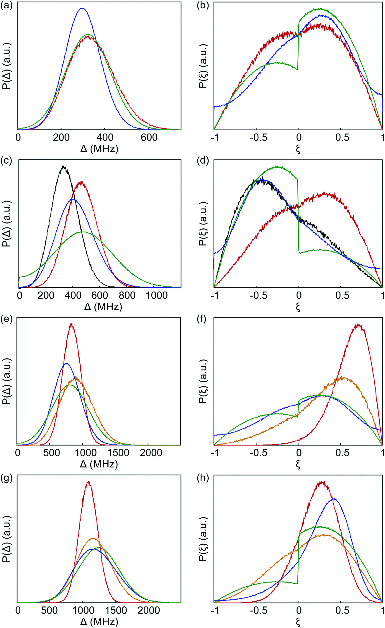 | ||
| Fig. 12 Comparison of distributions of anisotropy Δ (a, c, e and g) and axiality ξ (b, d, f and h) between fits to experimental data by Model 1 (blue) and Model 3 (green), as well as the prediction by superposition Model B with an isotropic standard deviation of atom positions σxyz = 0.05 Å (red). The orange curves are predictions by superposition Model B with an isotropic standard deviation of atom positions σxyz = 0.10 Å. (a and b) Gd-NO3Pic (1). (c and d) Gd-DOTA (2). The grey curves are predictions by superposition Model B based on the crystal structure of the Ce(III)-DOTA. (e and f) Gd-PyMTA (4). (g and h) Iodo-(Gd-PCTA-[12]) (6). The prediction for iodo-(Gd-PCTA12) is based on a crystal structure of the Ho(III) complex with a ligand that formally derives from PCTA-[12] by substitution of the carboxylate for phosphonate groups. | ||
For Gd-DOTA (2), the superposition Model B predicts the mean value of anisotropy Δ and thus of |D| quite well, but underestimates the standard distribution of anisotropy. More importantly, Model B predicts a wrong asymmetry of the axiality distribution P(ξ). The asymmetry of P(ξ) seen in Model 3 (green line in Fig. 12(d)) with stronger contributions at ξ < 0 than at ξ > 0 and in Model 1, where D = −600 MHz was used as a simulation input, is at least qualitatively correct, as it is in line with the asymmetry of the low-temperature G-band spectrum. Surprisingly, this asymmetry is nicely predicted by Model B if the crystal structure of Ce-DOTA instead of the one of Gd-DOTA (2) is used (grey line). Since all donor atoms are farther away from the lanthanide ion in the Ce-DOTA structure, a too small mean value is predicted for Δ. Although it may be possible to find a coordination polyhedron that leads to very good agreement between Models 3 and B, we refrain from this, since an arrangement of nine donor atoms cannot be uniquely determined from the information content in these distributions and since Model 3 is not perfect either.
Note also that the predictions by Model B based on the crystal structures of Gd-DOTA (2)52 and of the Gd-monoamide-DOTA49 that resembles Gd-maleimide-DOTA (3) differ significantly from each other. This difference can be traced back to a lengthening of the dative bond between Gd(III) ion and the oxygen atom of the carboxamide group by about 0.2 Å compared to a bond between a Gd(III) ion and a carboxylate oxygen atom and a concomitant slight shortening of the opposite dative bond.
For Gd-PyMTA, Model B predicts the mean value of the anisotropy quite well, but underestimates the width of the distribution (Fig. 12(e)). In particular, Model B with σxyz = 0.05 Å dramatically underestimates the width of the axiality distribution P(ξ) (Fig. 12(f)), which nicely agrees between Models 1 and 3. The deviation is significant, as the predicted distribution has significant contributions only from ξ > 0, which would cause a much stronger asymmetry of the low-temperature G-band spectrum than experimentally observed. This strongly suggests that for Gd-PyMTA the coordination geometry is less well defined than by a variation of the donor atom positions with σxyz = 0.05 Å with respect to their mean position in the crystal structure, as is assumed in Model B. This is plausible, since the position of the two coordinating water molecules is expected to vary more strongly in a frozen glassy solution. Note also that the crystal structure reported in ref. 50 features one Gd(III) center coordinated by only eight donor atoms. We tested this hypothesis by recomputing superposition Model B with σxyz = 0.10 Å (orange curves). Indeed, both the width of P(Δ) and the width and position of the maximum of P(ξ) are in much better agreement with the experimental results for this choice.
A similar trend as for Gd-PyMTA is observed for iodo-(Gd-PCTA-[12]) (6), albeit to a lesser extent (Fig. 12(g) and (h)). In addition, the mean value of the anisotropy is slightly underestimated. In this case, a simulation with σxyz = 0.10 Å and otherwise unchanged model parameters (orange lines in Fig. 12(g) and (h)) led to a very good agreement between the distribution predicted by ZFS Models 3 and superposition Model B, considering that Model 3 can mimic the asymmetry only by different vertical scaling of the ξ > 0 and ξ < 0 branches.
5.4 Predictions
When the crystal structure of a Gd(III) complex or the corresponding complex with another lanthanide(III) ion is known, the superposition model can be used for the prediction of ZFS values (Table 5). The values predicted by Model B with σxyz = 0.05 Å for an additional set of the seven Gd(III) complexes 8–14 shown in Fig. 13 are mostly within the range of the values measured in this work, with the exception of Gd-HAM2 for which a larger ZFS is predicted than for iodo-(Gd-PCTA-[12]). Note that the uncertainties of the predictions for Gd-EDTA and Gd-HAM2 may be particularly large because water coordination geometry is likely to differ in the crystal and in aqueous solution when three free coordination sites are available. In both crystal structures, three water molecules are coordinated with Gd(III)–O distances between and 2.416 and 2.530 Å (EDTA) and 2.319 and 2.384 Å (HAM2). In solution, on average longer and more varied Gd(III)–O(H2O) distances are to be expected, which would then lead to a larger mean ZFS magnitude. In both of these cases, one may also expect a larger standard deviation of the ZFS magnitude due to the larger variability of the donor atom coordinates for water ligands. We tested for this effect by repeating the computations for these two ligands with σxyz = 0.10 Å. For Gd-EDTA, this leads to an increase in from 528 to 838 MHz and in σ|D| from 154 to 273 MHz. For Gd-HAM2,
  increases only slightly from 2168 to 2276 MHz, while σ|D| more than doubles from 147 to 302 MHz. In general, one expects a larger effect on small
  upon increasing σxyz, since a small
  corresponds to a highly symmetric coordination polyhedron whose symmetry is rather sensitive to changes in the donor atom coordinates.

 | ||
| Fig. 13 Structural formulae and naming of the Gd(III) complexes 8–14 considered for ZFS parameter value prediction with the superposition Model B. | ||
6 Discussion
In this work, we determined the ZFS parameters D and E (or E/D) for a series of Gd(III) complexes by fitting three models for the ZFS parameter distributions to a set of multi-frequency EPR spectra acquired at Q-band (34 GHz), W-band (94 GHz), and G-band (240 GHz). The determined ZFS parameter values D and σD were found to be comparable within error across all three tested models if for Model 1 the dominant components of D and σD after reordering of the indices were taken into account. We find that the model proposed by Raitsimring et al., with the addition of an asymmetry parameter in the bimodal P(D) distribution (here, Model 3), provides a good compromise between a small number of fit parameters and a good match between the simulated and experimental EPR spectra.The combining of multi-frequency EPR data greatly enhances the confidence of the determined ZFS parameter values, as each measurement frequency provides slightly different information due to the varying contributions of the different EPR transitions at the different measurement frequencies and temperatures. In particular, the high-field and low-temperature G-band (240 GHz) spectra, whose lineshape is dominated by the |−7/2〉 → |−5/2〉 transition, was found to be crucial in determining the asymmetry of the bimodal P(D) distribution. However, inspection of the RMSD contour plots for Models 2 and 3 implies that a rough estimation of the ZFS parameters D and σD is possible with data at only a single measurement frequency in Q band or above. EPR spectra recorded in Q band and W band are rather insensitive to the asymmetry parameter P(+D)/P(−D) of Model 3, and so the lineshape can be adequately described under the assumption that the bimodal D distribution is symmetric about zero (i.e. Model 2).
The three phenomenological models tested in this work (Models 1–3) appear to be reasonable approximations of the ZFS parameter distributions, but they do not perfectly reproduce the experimental EPR spectra of the Gd(III) complexes. The systematic deviations between the best-fit simulations and the experimental data resulting from approximations taken in the models limit the precision with which we can determine ZFS parameter values, forcing us to set relatively large error bars for the D and σD values. The largest deviations for all three models are observed in the vicinity of the sharp central peak of the Gd(III) spectrum, resulting from an oversampling of values near D = 0 in the simulations. Adding a small intrinsic linewidth to broaden the region of the central peak in the Gd(III) spectrum was found to improve the agreement between the simulated and experimental EPR spectra (SI C.4, ESI†), perhaps by accounting for unresolved broadenings (i.e. hyperfine interactions, higher-order ZFS parameters, etc.) which are not included in the tested models and would be most visible as broadenings of the narrow central peak. However, it is difficult to introduce such a line broadening in a clear and systematic way into the global fits of multi-frequency EPR data and the physical interpretation of such a phenomenological parameter is ambiguous. For these reasons, it was found best to carry out normalization of the simulated spectra to the measured EPR data considering only the shoulders of the EPR spectra. This outer portion of the spectra is not sensitive to these extraneous broadening terms, while the height of the sharp central peak is highly sensitive to any additional broadening, and would thus bias an RMSD calculation if the spectra were normalized to the central peak.
The three tested models for the ZFS parameter distributions were found to produce simulated Gd(III) spectra that had small, but systematic, deviations from the measured EPR spectra resulting from approximations taken in the definition of the models. This necessitated the assignment of rather large error bars for the determined D and σD parameter values. In light of this, it is difficult to argue why the rigorous analysis performed here is necessary in every case where only an estimation of the ZFS parameter values for a Gd(III) complex is desired. It is tempting to simplify the fitting of ZFS parameter distributions to the mathematically ill-defined fit-by-eye approach. This manual fitting approach was conducted here for Models 1 and 3 (Section 4.1, SI N, ESI†) before the rigorous analysis was conducted, and was found to produce ZFS parameter values that fell-with one exception-within the conservatively defined error bars if for Model 1 the dominant component of D and σD after reordering of the indices were considered. The exception is the manually estimated D values for Gd-DOTA (2)/Gd-maleimide-DOTA (3) using Model 3, that lie within the error band of the RMSD analysis for the whole field range, but are out of the error band for the RMSD analysis excluding the central peak. Yet this method of fitting must be undertaken with caution, as the results are dependent on the physical intuition of the person performing the fit, and error bars cannot be assigned to the determined ZFS parameter values.
In this work we neglected a possible change of ZFS parameters between the measurement temperature of 5 K for G band and of 10 K for Q and W band. The best fit ZFS parameters vary between different microwave bands, indicating the approximate character of the ZFS models used in this work (ESI,† Tables F8 and F9). This variation exists between each two bands, and its magnitude seems to be uncorrelated with the temperature difference. Variations of ZFS with temperature were previously observed, for instance, for Mn(II) impurities in magnetically dense iron-based metalloorganic crystals60 and for a manganese superoxide dismutase,61 and were related to the sensitivity of zero-field interactions to metal–ligand distances and/or angular ligand positions. For the studied model Gd(III) complexes, we presume that the ligand sphere stays approximately constant in the studied temperature range. Note also, that, in the cited works, the variation of ZFS over a range of 5 K in the low temperature regime is very small compared to the accuracy of the presented ZFS determination and the widths of obtained ZFS parameter distributions.
Even given the conservative estimate of the accuracy of the D values for Gd(III) complexes determined in this work, the magnitude of the assigned error bars are still smaller than typical error bars from quantum chemical calculations of ZFS parameter values performed by standard computational approaches, which often fail to arrive at the correct sign or magnitude of the ZFS parameter values.62 This is one of the primary motivations for attempting to construct a semi-phenomenological model for ZFS parameter value predictions. The superposition model developed in this work, using known crystal structures of Gd(III) complexes as inputs, was found to qualitatively reproduce the ZFS parameter distribution described by Model 3. Furthermore, by assuming variation in donor atom coordinates consistent with Debye–Waller factors in crystal structures, the superposition Model B was successful in roughly estimating the magnitudes of D, distribution σD and the trends in the experimentally determined values. However, the ZFS parameter values determined by the superposition model lie slightly outside of the assigned error bars for some of the Gd(III) complexes studied here. Reproducing the distribution widths of D and of the axiality ξ require that different Debye–Waller factors are assumed for different ligands. For the DOTA ligand, the superposition model wrongly predicts an excess of configurations with positive ZFS if the crystal structure of Gd-DOTA is used, whereas it correctly predicts an excess of configurations with negative ZFS if the crystal structure of Ce-DOTA is used. This indicates that, at least for highly symmetric coordination polyhedra, subtle differences in donor atom coordinates can cause strong changes in the ZFS parameter distribution. The accuracy of predictions by the superposition model is thus limited if there are differences of the coordination polyhedra between crystal structures and solution. Furthermore, due to the relatively restricted set of input experimental data for calibration of the superposition model, it is currently difficult to estimate the strength of this model in predicting unknown ZFS parameter values for other Gd(III) complexes. Moreover, it was also observed in the above mentioned study on a manganese superoxide dismutase,61 that the superposition model of Newman and Urban63 for six- and four-coordinate d5 metal ions fails to predict the correct ZFS parameters in cases of high geometric asymmetry, indicating that some caution should be taken when applying the superposition model. Given the importance of accurate knowledge of ZFS parameter values for optimal design of particular EPR experiments and interpretation of data, this calls for additional work in this area-both in experimentally measuring ZFS parameter values for additional Gd(III) complexes and developing semi-phenomenological models relating the structure of the Gd(III) complex to the magnitude of the ZFS which will allow for the design of tailored Gd(III) complexes.
Nevertheless, the work presented here, allows to give some general comments on the current state of ZFS analysis in Gd(III) complexes, and on the capability of the existing methods to relate spectroscopic parameters to the metal–ligand chemical bonding. The superposition model relates the widths of D and E distributions to variations in the metal complex structure. In the earlier work of Raitsimring and colleagues, reorientations of the ligands around the central Gd(III) ion, with constant interatomic distances, were assumed. In the present work, we rather approximate ligand position variations as isotropic narrow Gaussian distributions in a 3D space, according to the X-ray Debye–Waller factors, and allow different strength of ZFS contributions from oxygen and nitrogen atoms. Fitting of the superposition model to the set of experimental data suggests that nitrogen ligands have about 8% stronger contributions to ZFS than oxygen ligands. It appears that both Raitsimring's and our assumptions lead to very similar types of D and E distributions, which cannot be unambiguously discriminated even by the rigorous analysis of multi-frequency EPR data. Hence, it is difficult to say with confidence if ZFS distributions originate mainly from metal–ligand distance variations, from orientational distributions of the ligands around the metal ion, or from both these factors. The superposition model assumes that the same type of ligating atom (in our case, oxygen or nitrogen) gives the same distance-dependent contribution to the total ZFS. This is an approximation, which does not perfectly describe the presented experimental data, but it correctly catches the overall ZFS variation trend. Since currently accurate quantum chemical calculations for Gd(III) are not available, it would be difficult to relate the observed ZFS values to some deeper details of the chemical bonding at e.g. molecular orbital level. While some speculations on a case-by-case basis might still be possible, such speculations are beyond the scope of this work. It would be very helpful to generate a library of ZFS data on different Gd(III) centers, including Gd-EDTA and Gd-DOTAM as examples for small ZFS and scan this large experimental data set for such relations.
7 Conclusions
We made an extensive attempt to verify the accuracy of the determination of ZFS parameters and their distributions from multi-frequency EPR data. We discussed the relation between the two most commonly used models for the ZFS parameter distributions: (1) the model proposed by Benmelouka et al.,24 which assumes that the distributions of D and E are described by uncorrelated Gaussian distributions, and (2) the model proposed by Raitsimring et al., which takes the distribution of D to be a bimodal Gaussian distribution centered about D = 0 and the distribution of P(E/D) to be described by the polynomial expression P(E/D) ∝ (E/D) − 2·(E/D)2. We additionally investigated a third model, in which we allowed for an asymmetry of the bimodal D distribution of Model 2. We found that the distribution described by Model 1 could lead to an inconsistency with the typical definitions of the ZFS parameter values D and E. This inconsistency can be easily corrected and the ZFS parameter distributions recomputed, resulting in distributions rather similar to those described by Model 3. We additionally showed that the predicted D and σD values are consistent between the three models. The value of D is reasonably well constrained by fitting with these models, but the σD and asymmetry parameter P(+D)/P(−D) are much less well constrained. The use of multi-frequency EPR data increased the confidence of the determination of ZFS parameters, with high-field low-temperature spectra being crucial for determination of the asymmetry parameter P(+D)/P(−D) and the sign of D. In our opinion, the model proposed by Raitsimring et al.,23 with the addition of an allowance for asymmetry of the bimodal D distribution, appears to provide the most adequate description of ZFS distributions for Gd(III) complexes in frozen glassy solutions.Finally, we proposed an extension to the superposition model for the prediction of ZFS parameters, which allowed for reproduction of the trends in the strength of the ZFS for different Gd(III) complexes and rough estimation of the magnitude of D. This extended superposition model may be useful in estimating the strength of ZFS for Gd(III) complexes, e.g. based on optimized geometry calculations, which are typically more accurate than quantum chemical ZFS calculations. While this approach cannot be expected to predict exact ZFS parameters, it may provide a reasonable guideline for the selection of a Gd(III) complex for experiments in which the strength of ZFS is important (e.g., Gd(III) complexes with weak, intermediate or strong ZFS), and, thus, help to design tailored Gd(III) complexes prior to any synthesis efforts.
Author contributions
AG, SH, GJ, MSS, and MY designed the research. MQ, JW, VK and HH synthesized the Gd(III) complexes under the supervision of AG. KK performed the EPR measurements in Q and W band, worked on the convergence criteria for all models, and performed calculations relating to Model 1 under supervision of MY and GJ. JAC performed the 240 GHz EPR measurements and the RMSD calculations relating to Models 2 and 3, under the supervision of MSS and SH. GJ performed the analysis with the superposition models. All authors analyzed the experimental and computational results for all models, and contributed to writing the manuscript.Conflicts of interest
There are no conflicts to declare.Acknowledgements
This work was supported by funding from the Swiss National Science Foundation (200020_169057), the NSF (Molecular and Cellular Biology grants MCB-1244651 and MCB-1617025), the NIH (R01GM116128) and the Deutsche Forschungsgemeinschaft SPP1601 (GO555/6-2). We acknowledge support from the Center for Scientific Computing from the CNSI, MRL: an NSF MRSEC (DMR 1720256) and NSF CNS-0960316, and thank Miriam Hülsmann for support in the synthesis.References
- D. Goldfarb, Gd3+ spin labeling for distance measurements by pulse EPR spectroscopy, Phys. Chem. Chem. Phys., 2014, 16, 9669–10234 RSC.
- M. Yulikov, Spectroscopically orthogonal spin labels and distance measurements in biomolecules, in Electron Paramagnetic Resonance, ed. B. Gilbert, V. Chechik and D. Murphy, 2015, vol. 24, pp. 1–31 Search PubMed.
- A. Feintuch, G. Otting and D. Goldfarb, Gd3+ Spin Labeling for Measuring Distances in Biomacromolecules: Why and How?, Methods in Enzymology, 2015, vol. 563, pp. 415–457 Search PubMed.
- E. H. Abdelkader, X. Yao, A. Feintuch, L. A. Adams, L. Aurelio, B. Graham, D. Goldfarb and G. Otting, Pulse EPR-enabled interpretation of scarce pseudocontact shifts induced by lanthanide binding tags, J. Biomol. NMR, 2016, 64, 39–51 CrossRef CAS PubMed.
- E. A. Suturina, D. Häussinger, K. Zimmermann, L. Garbuio, M. Yulikov, G. Jeschke and I. Kuprov, Model-free extraction of spin label position distributions from pseudocontact shift data, Chem. Sci., 2017, 8, 2751–2757 RSC.
- J.-C. G. Bnzli, Lanthanide luminescence for biomedical analyses and imaging, Chem. Rev., 2010, 110, 2729–2755 CrossRef PubMed.
- E. Debroye and T. N. Parac-Vogt, Towards polymetallic lanthanide complexes as dual contrast agents for magnetic resonance and optical imaging, Chem. Soc. Rev., 2014, 43, 8178–8192 RSC.
- J. G. Reifernberger, P. Ge and P. R. Selvin, Progress in Lanthanides as Luminescent Probes, in Reviews in Fluorescence, ed. C. D. Geddes and J. R. Lakowicz, Springer, US, 2005, pp. 399–431 Search PubMed.
- A. Abragam and B. Bleaney, Electron paramagnetic resonance of transition ions, Clarendon Press, 1970 Search PubMed.
- S. Cotton, Lanthanide and Actinide Chemistry MODULE 4005 Organometallic Chemistry of Lanthanides, Wiley, 2006 Search PubMed.
- D. Newman and W. Urban, Interpretation of S-state ion E.P.R. spectra, Adv. Phys., 1975, 24, 793–844 CrossRef CAS.
- A. Dalaloyan, M. Qi, S. Ruthstein, S. Vega, A. Godt, A. Feintuch and D. Goldfarb, Gd(III)–Gd(III) EPR distance measurements- the range of accessible distances and the impact of zero field splitting, Phys. Chem. Chem. Phys., 2015, 17, 18464–18476 RSC.
- M. Ramirez-Cohen, V. Frydman, P. Milko, M. A. Iron, E. H. Abdelkader, M. D. Lee, J. D. Swarbrick, A. Raitsimring, G. Otting, B. Graham, A. Feintuch and D. Goldfarb, Overcoming artificial broadening in Gd3+–Gd3+ distance distributions arising from dipolar pseudo-secular terms in DEER experiments, Phys. Chem. Chem. Phys., 2016, 18, 12847–12859 RSC.
- A. Collauto, V. Frydman, M. D. Lee, E. H. Abdelkader, A. Feintuch, J. D. Swarbrick, B. Graham, G. Otting and D. Goldfarb, RIDME distance measurements using Gd(III) tags with a narrow central transition, Phys. Chem. Chem. Phys., 2016, 19037–19049 RSC.
- K. Keller, V. Mertens, M. Qi, A. Nalepa, A. Godt, A. Savitsky, G. Jeschke and M. Yulikov, Computing Distance Distributions from Dipolar Evolution Data with Overtones: RIDME Spectroscopy with Gd(III)-Based Spin Labels, Phys. Chem. Chem. Phys., 2017, 17856–17876 RSC.
- A. Doll, M. Qi, S. Pribitzer, N. Wili, M. Yulikov, A. Godt and G. Jeschke, Sensitivity enhancement by population transfer in Gd(III) spin labels, Phys. Chem. Chem. Phys., 2015, 17, 7334–7344 RSC.
- M. Yulikov, P. Lueders, M. Farooq Warsi, V. Chechik and G. Jeschke, Distance measurements in Au nanoparticles functionalized with nitroxide radicals and Gd3+–DTPA chelate complexes, Phys. Chem. Chem. Phys., 2012, 14, 10732 RSC.
- P. Lueders, H. Jager, M. A. Hemminga, G. Jeschke and M. Yulikov, Distance measurements on orthogonally spin-labeled membrane spanning WALP23 polypeptides, J. Phys. Chem. B, 2013, 117, 2061–2068 CrossRef CAS PubMed.
- J. A. Clayton, M. Qi, A. Godt, D. Goldfarb, S. Han and M. S. Sherwin, Gd3+–Gd3+ distances exceeding 3 nm determined by very high frequency continuous wave electron paramagnetic resonance, Phys. Chem. Chem. Phys., 2017, 19, 5127–5136 RSC.
- A. M. Raitsimring, C. Gunanathan, A. Potapov, I. Efremenko, J. M. L. Martin, D. Milstein and D. Goldfarb, Gd3+ complexes as potential spin labels for high field pulsed EPR distance measurements, J. Am. Chem. Soc., 2007, 129, 14138–14139 CrossRef CAS PubMed.
- A. Raitsimring, A. Dalaloyan, A. Collauto, A. Feintuch, T. Meade and D. Goldfarb, Zero field splitting fluctuations induced phase relaxation of Gd3+ in frozen solutions at cryogenic temperatures, J. Magn. Reson., 2014, 248, 71–80 CrossRef CAS PubMed.
- A. Lasoroski, R. Vuilleumier and R. Pollet, Vibrational dynamics of zero-field-splitting hamiltonian in gadolinium-based MRI contrast agents from ab initio molecular dynamics, J. Chem. Phys., 2014, 141, 014201 CrossRef PubMed.
- A. M. Raitsimring, A. V. Astashkin, O. G. Poluektov and P. Caravan, High-Field Pulsed EPR and ENDOR of Gd3+ Complexes in Glassy Solutions, Appl. Magn. Reson., 2005, 28, 281–295 CrossRef CAS.
- M. Benmelouka, J. Van Tol, A. Borel, M. Port, L. Helm, L. C. Brunel and A. E. Merbach, A High-Frequency EPR Study of Frozen Solutions of Gd(III) Complexes: Straightforward Determination of the Zero-Field Splitting Parameters and Simulation of the NMRD Profiles, J. Am. Chem. Soc., 2006, 128, 7807–7816 CrossRef CAS PubMed.
- H. A. Buckmaster and Y. H. Shing, A survey of the EPR spectra of Gd3+ in single crystals, Phys. Status Solidi A, 1972, 12, 325–361 CrossRef CAS.
- A. M. Raitsimring, A. V. Astashkin and P. Caravan, High-frequency EPR and ENDOR characterization of MRI contrast agents, in Biological Magnetic Resonance, ed. L. Berliner and G. Hanson, Springer, New York, 2009, pp. 581–621 Search PubMed.
- W. Blumberg, The EPR of high spin Fe3+ in rhombic fields, Magnetic resonance in biological systems, ed. A. Ehrenberg, B. G. Malmstrm and T. Vnngrd, Pergamon, Oxford, 1967, pp. 119–133 Search PubMed.
- M. Azarkh and E. J. Groenen, Simulation of multi-frequency EPR spectra for a distribution of the zero-field splitting, J. Magn. Reson., 2015, 255, 106–113 CrossRef CAS PubMed.
- W. R. Hagen, Wide zero field interaction distributions in the high-spin EPR of metalloproteins, Mol. Phys., 2007, 105, 2031–2039 CrossRef CAS.
- J. T. Weisser, M. J. Nilges, M. J. Sever and J. J. Wilker, EPR Investigation and Spectral Simulations of Iron Catecholate Complexes and Iron Peptide Models of Marine Adhesive Cross-Links, Inorg. Chem., 2006, 45, 7736–7747 CrossRef CAS PubMed.
- A. P. Golombek and M. P. Hendrich, Quantitative analysis of dinuclear manganese(II) EPR spectra, J. Magn. Reson., 2003, 165, 33–48 CrossRef CAS PubMed.
- G. Scholz, R. Stsser, M. Krossner and J. Klein, Modelling of multifrequency ESR spectra of Fe3+ ions in crystalline and amorphous materials: a simplified approach to determine statistical distributions of spin–spin coupling parameters, Appl. Magn. Reson., 2001, 21, 105–123 CrossRef CAS.
- E. M. Yahiaoui, R. Berger, Y. Servant, J. Kliava, L. Cugunov and A. Mednis, Electron paramagnetic resonance of Fe3+ ions in borate glass: computer simulations, J. Phys.: Condens. Matter, 1994, 6, 9415 CrossRef CAS.
- A. Yang and B. Gaffney, Determination of relative spin concentration in some high-spin ferric proteins using E/D-distribution in electron paramagnetic resonance simulations, Biophys. J., 1987, 51, 55–67 CrossRef CAS PubMed.
- M. Benmelouka, J. Van Tol, A. Borel, S. Nellutla, M. Port, L. Helm, L. C. Brunel and A. E. Merbach, Multiple-frequency and variable-temperature EPR study of gadolinium(III) complexes with polyaminocarboxylates: analysis and comparison of the magnetically dilute powder and the frozen-solution spectra, Helv. Chim. Acta, 2009, 92, 2173–2185 CrossRef CAS.
- I. Gromov, J. Shane, J. Forrer, R. Rakhmatoullin, Y. Rozentzwaig and A. Schweiger, A Q-band pulse EPR/ENDOR spectrometer and the implementation of advanced one- and two-dimensional pulse EPR methodology, J. Magn. Reson., 2001, 149, 196–203 CrossRef CAS PubMed.
- R. Tschaggelar, B. Kasumaj, M. G. Santangelo, J. Forrer, P. Leger, H. Dube, F. Diederich, J. Harmer, R. Schuhmann, I. García-Rubio and G. Jeschke, Cryogenic 35 GHz pulse ENDOR probehead accommodating large sample sizes: performance and applications, J. Magn. Reson., 2009, 200, 81–87 CrossRef CAS PubMed.
- Y. Polyhach, E. Bordignon, S. Gandra, A. Godt and G. Jeschke, High sensitivity and versatility of the DEER experiment on nitroxide radical pairs at Q-band frequencies, Phys. Chem. Chem. Phys., 2012, 14, 10762–10773 RSC.
- S. Takahashi, L.-C. Brunel, D. T. Edwards, J. Van Tol, G. Ramian, S. Han and M. S. Sherwin, Pulsed electron paramagnetic resonance spectroscopy powered by a free-electron laser, Nature, 2012, 489, 409–413 CrossRef CAS PubMed.
- D. T. Edwards, Z. Ma, T. J. Meade, D. Goldfarb, S. Han and M. S. Sherwin, Extending the distance range accessed with continuous wave EPR with Gd3+ spin probes at high magnetic fields, Phys. Chem. Chem. Phys., 2013, 15, 11313–11326 RSC.
- M. Weger, Passage Effects in Paramagnetic Resonance Experiments, Bell Syst. Tech. J., 1960, 39, 1013–1112 CrossRef.
- A. Portis, Rapid passage effects in electron spin resonance, Phys. Rev., 1955, 100, 1219–1221 CrossRef CAS.
- W. Low, Paramagnetic Resonance Spectrum of Manganese in Cubic MgO and GaF, Phys. Rev., 1957, 105, 793–800 CrossRef CAS.
- V. I. Krinichnyi, Investigation of biological systems by high resolution 2 mm wave band ESR, J. Biochem. Biophys. Methods, 1991, 23, 1–30 CrossRef CAS PubMed.
- S. Stoll and A. Schweiger, EasySpin, a comprehensive software package for spectral simulation and analysis in EPR, J. Magn. Reson., 2006, 178, 42–55 CrossRef CAS PubMed.
- A. V. Astashkin and A. M. Raitsimring, Electron spin echo envelope modulation theory for high electron spin systems in weak crystal field, J. Chem. Phys., 2002, 117, 6121–6132 CrossRef CAS.
- L. Garbuio, K. Zimmermann, D. Häussinger and M. Yulikov, Gd(III) complexes for electron–electron dipolar spectroscopy: effects of deuteration, pH and zero field splitting, J. Magn. Reson., 2015, 259, 163–173 CrossRef CAS PubMed.
- C. Gateau, M. Mazzanti, J. Pécaut, F. A. Dunand and L. Helm, Solid-state and solution properties of the lanthanide complexes of a new nonadentate tripodal ligand derived from 1,4,7-triazacyclo-nonane, Dalton Trans., 2003, 2428–2433 RSC.
- S. Aime, P. Anelli, M. Botta, F. Fedeli, M. Grandi, P. Paoli and F. Uggeri, Gd(III) Complexes of DOTA-like Ligand Derivatives, Inorg. Chem., 1992, 31, 2422–2428 CrossRef CAS.
- C. Gunanathan, Y. Diskin-Posner and D. Milstein, Lanthanide Organic Framework of a Rigid Bis-Gd Complex: Composed by Carbonate Ions Spacers, Cryst. Growth Des., 2010, 10, 4235–4239 CAS.
- M. Le Fur, M. Beyler, N. Lepareur, O. Fouge, C. Platas-Iglesias, O. Rousseaux and R. L. Tripier, Pyclen Tributylphosphonate ester as potential chelator for targeted radiotherapy: from Yttrium(III) complexation to 90Y radiolabeling, Inorg. Chem., 2016, 55, 8003–8012 CrossRef CAS PubMed.
- C. A. Chang, L. C. Francesconi, M. F. Malley, K. Kumar, J. Z. Gougoutas, M. F. Tweedle, D. W. Lee and L. J. Wilson, Synthesis, Characterization, and Crystal Structures of M(DO3A) (M = Iron, Gadolinium) and Na[M(DOTA)] (M = Fe, Yttrium, Gd), Inorg. Chem., 1993, 32, 3501–3508 CrossRef CAS.
- F. Benetollo, G. Bombieri, L. Calabi, S. Aime and M. Botta, Structural Variations Across the Lanthanide Series of Macrocyclic DOTA Complexes: Insights into the Design of Contrast Agents for Magnetic Resonance Imaging, Inorg. Chem., 2003, 19, 1319 Search PubMed.
- G. Bombieri, N. Marchini, S. Ciattini, A. Mortillaro and S. Aime, The crystallized solvent could influence the lanthanide water bonding?, Inorg. Chim. Acta, 2006, 359, 3405–3411 CrossRef CAS.
- L. K. Templeton, D. H. Templeton, A. Zalkin and H. W. Ruben, Anomalous scattering by praseodymium, samarium and gadolinium and structures of their ethylenediaminetetraacetate (edta) salts, Acta Crystallographica Section B Structural Crystallography and Crystal, Chemistry, 1982, 38, 2155–2159 Search PubMed.
- A. Bianchi, L. Calabi, C. Giorgi, P. Losi, P. Mariani, P. Paoli, P. Rossi, B. Valtancoli and M. Virtuani, Thermodynamic and structural properties of Gd3+ complexes with functionalized macrocyclic ligands based upon 1,4,7,10-tetraazacyclododecane, J. Chem. Soc., Dalton Trans., 2000, 697–705 RSC.
- L. S. Natrajan, N. M. Khoabane, B. L. Dadds, C. A. Muryn, R. G. Pritchard, S. L. Heath, A. M. Kenwright, I. Kuprov and S. Faulkner, Probing the structure, conformation, and stereochemical exchange in a family of lanthanide complexes derived from tetrapyridyl-appended cyclen, Inorg. Chem., 2010, 49, 7700–7709 CrossRef CAS PubMed.
- M. S. Konings, W. C. Dow, D. B. Love, K. N. Raymond, S. C. Quay and S. M. Rocklage, Gadolinium complexation by a new DTPA-amide ligand. Amide oxygen coordination, Inorg. Chem., 1990, 29, 1488–1491 CrossRef CAS.
- S. W. A. Bligh, N. Choi, E. G. Evagorou, M. Mcpartlin, W. J. Cummins and J. D. Kelly, Synthesis and crystal structure of a gadolinium(III) complex of a tetraimine schiff-base macrocycle: a potential contrast agent for magnetic resonance imaging, Polyhedron, 1992, 11, 2571–2573 CrossRef CAS.
- H. Daubric, J. Kliava, P. Guionneau, D. Chasseau, J.-F. Ltard and O. Kahn, Spin transition in [Fe(PM-BiA)2(NCS)2] studied by the electron paramagnetic resonance of the Mn2+ ion, J. Phys.: Condens. Matter, 2000, 12, 5481 CrossRef CAS.
- L. C. Tabares, N. Cortez, I. Agalidis and S. Un, Temperature-Dependent Coordination in E. coli Manganese Superoxide Dismutase, J. Am. Chem. Soc., 2005, 127, 6039–6047 CrossRef CAS PubMed.
- T. Gupta and G. Rajaraman, Modelling spin Hamiltonian parameters of molecular nanomagnets, Chem. Commun., 2016, 8972, 8972–9008 RSC.
- D. J. Newman and W. Urban, Interpretation of S-state ion E.P.R. spectra, Adv. Phys., 1975, 24, 793–844 CrossRef CAS.
Footnotes |
| † Electronic supplementary information (ESI) available. See DOI: 10.1039/c7cp08507a |
| ‡ These authors contributed equally. |
| This journal is © the Owner Societies 2018 |