Yield prediction in parallel homogeneous assembly

Abstract

We investigate the parallel assembly of two-dimensional, geometrically-closed modular target structures out of homogeneous sets of macroscopic components of varying anisotropy. The yield predicted by a chemical reaction network (CRN)-based model is quantitatively shown to reproduce experimental results over a large set of conditions. Scaling laws for parallel assembling systems are then derived from the model. By extending the validity of the CRN-based modelling, this work prompts analysis and solutions to the incompatible substructure problem.

---

1 Introduction

Large-scale manufacturing requires fast and efficient fabrication of many exact copies of desired objects. Robot assisted fabrication typically involves serial, deterministic procedures that are reliable but inefficient to assemble vast quantities of products, especially those of small size.^1,2 An alternative manufacturing strategy consists of components assembling with one another autonomously to form many equal copies of a target structure. Such a self-assembly approach³ is massively parallel and inspired by natural systems that assemble autonomously, such as crystals⁴ and viruses.⁵

A set of mobile components capable of bonding with one another will tend to form assemblies in a bounded space. The formation of intercomponent bonds decreases the enthalpy of the system⁶ and the number of accessible component configurations.⁷ Under thermal conditions that make entropic contributions negligible, the assembly of components reduces the free energy of the system, as well as the number of further bonds that can be formed. However, modular assembling systems are characterised by a multitude of intermediate states, associated with local minima in the free energy landscape, besides a few degenerate target states that correspond to global minima.⁸ Assembling systems able to break out of local energy minima, thanks to, e.g., perturbing energy imparted to the system to compete with bond formation, are self-assembling systems.^9,10 Assembling systems incapable of escaping local energy minima in finite time are aggregating systems.¹¹ Irreversible intercomponent bonds arrest aggregating systems typically within one of their local energy minima. Once in a local minimum, aggregating systems are prevented from exploring further possible configurations to reach the target state(s). Self-assembly is often used in literature, albeit incorrectly, to describe aggregating systems as well.¹⁰ In the following, we use assembly to describe systems that aggregate.

An assembling system is in a depletion trap when no more components are available to advance the assembly, as all components are already employed in existing (sub)structures.¹² In parallel assembling systems of homogeneous components, depletion traps are absorbing states of the dynamics and local energy minima corresponding to the formation of incompatible substructures, i.e., partial target structures which cannot complete assembly due to steric incompatibility.§Fig. 1 illustrates an instance of the issue. By preventing the assembly of target structures, the formation of incompatible substructures significantly reduces the assembly yield in parallel homogeneous assembly, and therefore wastes resources.¹⁶ At the same time, the incompatible substructure problem is both a logical and a physical problem, and is thus amenable to both analytical and experimental study.

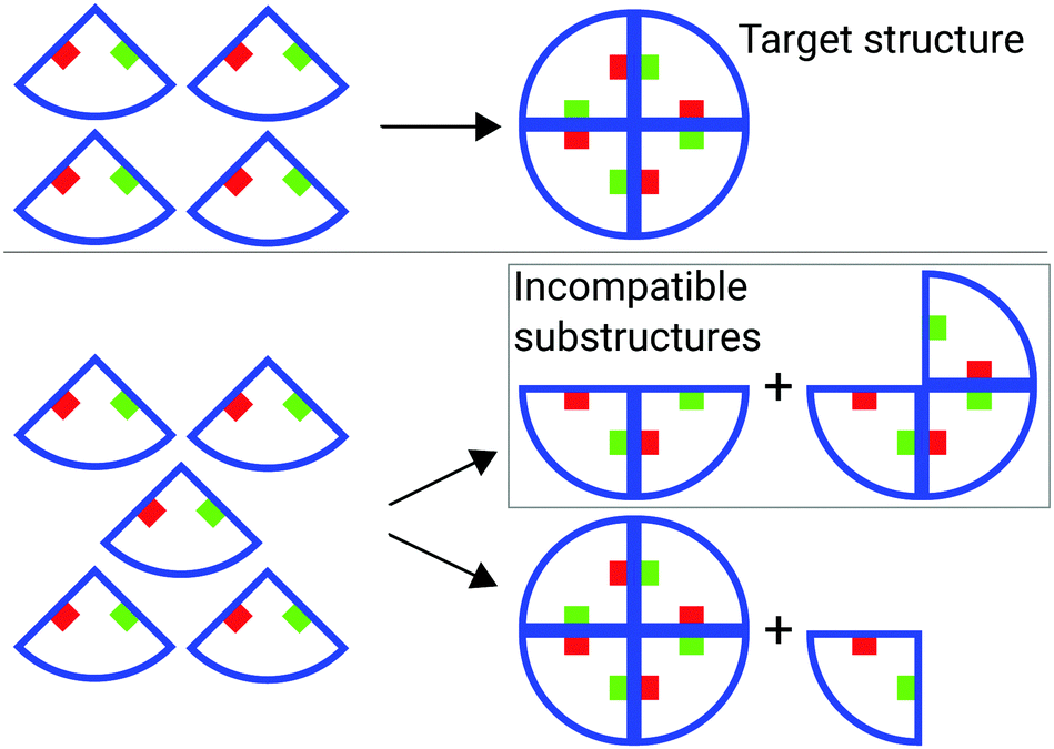Fig. 1 An instance of the incompatible substructure problem in the assembly of a modular target structure. The circular target structure is composed of 4 equal sector-shaped components. In an aggregating system, each of the available components moves within a confined space and irreversibly bonds with two components. When exactly 4 components are used, a single target structure will always assemble. However, 5 components will not always form a single target structure and a spare component, i.e., a {1,4} population. They could instead end in one of 2 absorbing states—the other one being {2,3}.

In this paper, we present a comprehensive study of model-based prediction of assembly yield for parallel assembling systems. We consider the parallel assembly of two-dimensional (2D), geometrically-closed target structures composed of homogeneous sectors of varying anisotropy. The results of an extensive set of parametric assembly experiments are quantitatively shown to closely match in most cases the assembly yield predictions obtained by a corresponding chemical reaction network (CRN)-based model. Consequently, this work significantly extends the validity of CRN-based modelling of assembling systems, and the analysis of the incompatible substructure problem provides a foundation for the study of dynamical aspects of parallel (self)-assembly.

The paper is organised as follows. Section 2 gives an account of prior art. The physical system and the CRN-based model used in this study are described respectively in Sections 3 and 4. The experiments conducted to compare the physical system and analytical model are presented in Section 5. The results are reported in Section 6. Scaling of system properties is discussed in Section 7. Finally, Section 8 provides conclusions and outlook.

2 Background

The study of agents coming together to form autonomously ordered predictable and structures has been pioneered in the context of molecular chemistry,^17,18 biology,¹⁹ material sciences¹⁷ and soft matter.²⁰ A seminal paper by Penrose and Penrose²¹ presented a macroscopic mechanical assembling system. In the early 1980's, a model of diffusion-limited aggregation was proposed by Witten Jr. and Sander.¹¹ By the early 2000's, self-assembly was acknowledged as a self-standing multidisciplinary field of study,^3,9,10 and several macroscopic analogues have been designed to elucidate or imitate microscopic assembly processes.^22–26

In the context of parallel assembly, Hosokawa et al.²⁷ studied the assembly of triangular components into hexagonal target structures. Hosokawa et al. described the negative impact of incompatible substructures on assembly yield in their experiments, and first proposed to study their parallel assembly system using the formalism of chemical reaction networks.

Klavins²⁸ built a mechatronic version of the triangular components used by Hosokawa et al.²⁷ Software embedded in their “programmable parts” defined rules, based on graph grammars, to guide the assembly of specified target structures. The programmability of the components was used to control the interactions, leading to coordinated behaviour of the system—an approach recently extended by Haghighat and Martinoli.²⁹

Miyashita et al.³⁰ studied the influence of reversible reactions on the yield of an assembly system. Their latching self-propelled components floated on the surface of water and had similar shape to those of Hosokawa et al.²⁷ Miyashita et al. conducted experiments to compare sequential aggregation, reversible assembly and random aggregation using these components. They used a CRN-based model to quantitatively describe their system.

Mermoud et al.³¹ and Haghighat et al.³² developed a magneto-fluidic system of passive, centimetre-sized components that self-assembled on water. The system was supported by a general, CRN-based, multi-level modelling framework for stochastic distributed systems of reactive agents. Using such framework, the authors were able to control the self-assembly of the water-floating components in real-time. Mastrangeli et al.³³ developed a downscaled version of the system, tailored for the automated control of the acousto-fluidic self-assembly of microparticles.

Hacohen et al.³⁴ proposed an algorithm to program the mechanical self-assembly of 3D macroscale objects. Taking inspiration from the fully specified assembly of DNA-based structures, Hacohen et al. showed that an arbitrary 3D object, properly dissected into components, can be re-assembled by unsupervised mechanical shaking when appropriate rules are uniquely encoded on the faces of the components. In their experiments, Hacohen et al. introduced enough components to assemble 2 target structures of 18 components in parallel, and were able to assemble only 1 target structure with no erroneous bonds.

Murugan et al.¹² studied the formation of incompatible substructures in chemical reaction-based systems. Using a theoretical model relevant to DNA, proteins and colloids, the authors suggested that the incidence of incompatible substructures can be reduced by appropriately tuning the reaction rates by the stoichiometry of the system.

Borrowing the concepts of intercomponent bond and structure formation from chemical reactions, CRN-based formalisms and approaches³⁵ are commonly used to model and simulate aggregating and self-assembling systems. However, experimental validation of CRN-based model predictions of assembly yield is, to date, mostly qualitative. For instance, Hosokawa et al.²⁷ conducted a single experiment under 2 conditions (systems of 20 and 100 components) and 100 trials per condition, while Miyashita et al.³⁰ conducted a single experiment under 2 conditions (systems of 6 and 7 components) with 10 trials per condition. While noteworthy demonstrations of the feasibility of CRN-based modeling, these contributions fall short of showing the details of the relationship between the CRN-based model and physical experiments. Such a lack of comprehensive and quantitative comparison motivates the work presented here.

3 Physical system

We study the assembly yield of a two-dimensional system of passive components designed to form geometrically-closed target structures. The components are agitated within a reactor that is a bounded horizontal container attached to an orbital shaker. The agitation enables components and substructures to move around the reactor, interact with one another, and form irreversible magnetic bonds. Substructures of the target structures assemble upon bond formation. Only geometrically compatible substructures can bond together, eventually forming full target structures. The target structures are by design inert and stop growing once formed.

Components

All components are 3D-printed, 7 mm-thick polyhedra embedding magnets with opposite orientations in two of their faces to enforce the formation of the closed target structures (Fig. 2). NdFeB magnets (N48, Supermagnete (Webcraft GmbH), strength 210 g) assure intercomponent bonds that can withstand impacts with the container and among components.

Fig. 2 The 3D printed components with embedded magnets used in the experiments (dimensions overlaid). Positions and orientations of the magnets are marked.

We designed target structures of equal area and three different shapes: circle, square and triangle. All component sets are homogeneous. Sectors of a circle with radius 25 mm compose the circular target structures. We use sets of sector-shaped components with 4 different sector angles: 45°, 60°, 72° and 90°. Magnets are embedded in the middle of the two straight faces. For square target structures, the components are 4 equal squares with side length of 22.2 mm, with magnets embedded in two adjacent lateral faces. For triangular target structures, the components are 3 identical isosceles triangles, the two equal sides and the base side measuring 38 mm and 67 mm, respectively. Magnets are embedded in the middle of the two equal sides.

Reactor

The experiments were carried out in a lid-covered circular container of inner radius of 125 mm, bounded by a 9 mm-thick rim (Fig. 3). The container and the lid, made from clear acrylic, were fastened to an orbital shaker (New Brunswick™ Innova® 2300). The reactor served two purposes: (1) to transfer kinetic energy from the shaker to the components, and (2) to constrain the component motion in 2D and avoid component flipping. We chose the components density in the reactor so that the components could frequently interact with one another while minimizing packing effects and avoiding jamming of the (sub)structures (e.g., 5 target structures occupied 20% of the reactor surface). We set the shaker frequency depending on the experiment type to maximise interactions among substructures while avoiding disassembly events. Orbital shaking produced a qualitatively pseudo-random motion of the components. The experimental results are not expected to be significantly influenced by the shaking method.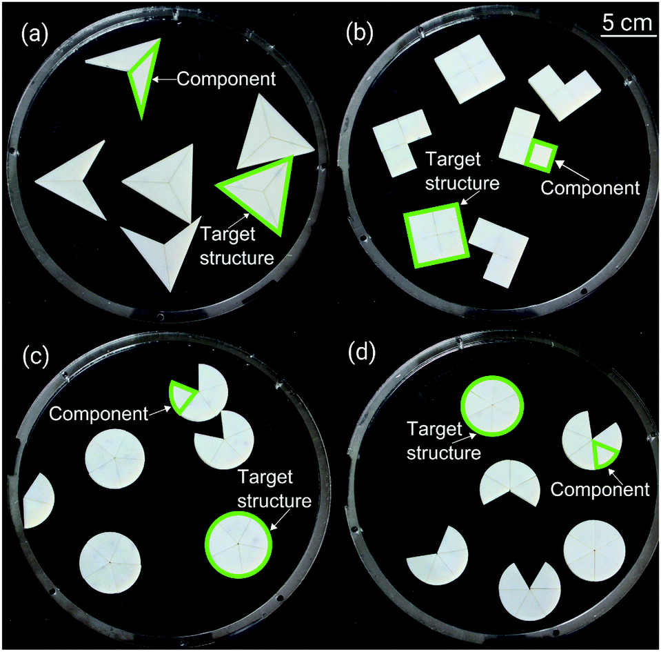

Fig. 3 Absorbing states from four different physical assembly trials: (a) triangular, (b) square, (c) 72° sector and (d) 60° sector components. The exact number of components to form 5 target structures was provided in all samples.

4 Analytical model

We analyse our assembling system with the chemical reaction network-based model proposed by Hosokawa et al.²⁷ In the model, the population of the system is represented as a multiset of integers, x_i. The integer x_i represents the number of substructures with i, 1 ≤ i ≤ N, components and N the number of components in a full target structure. X_i represents a substructure with i components. Considering, for instance, a system with N = 8 equal components¶ shaped as 45° sectors to form a circular target structure, the state vector is x = (x₁,…,x₈). As we are excluding reverse reactions through irreversible intercomponent bonds, the state of the 45°-sector system can undergo the following set of reactions:

Given a large enough population, we study the probabilistic evolution of the system using a system of difference equations:

x(t + 1) = x(t) + F(x(t))

where t is the number of bond forming collisions between clusters, and the transition function is F = (F₁,…,F₈). The number F_i represents the expected value for each incremental step of x_i, and it is the summation of the stoichiometric coefficient v_ij times the probability P_j with which the jth reaction in eqn (1) occurs, i.e., . An example of the calculation is presented in Section 3.1 of Hosokawa et al.²⁷ The probability P_j is the product of the collision probability and bonding probability, P_j = P^c_lmP^b_lm. When x ≫ 1, the collision probability is defined as:
where , i.e., the total number of clusters.

The geometry-specific values of P^b are calculated according to Hosokawa et al.²⁷ We implement the calculation by placing the first substructure at the origin and the second substructure at infinity. The faces of the components form an angle of visibility. The number P^b is the probability that the angle of visibility of one substructure's face that includes the South polarity magnet (refer to Fig. 2) is within the angle of visibility of another substructure's face that includes the North polarity magnet. A more detailed explanation of the computation is available in Appendix A of Hosokawa et al.²⁷ The values of P^b used in this work are presented in Table 1.

Table 1 Assembly reactions and corresponding bonding probabilities P^b for chemical reaction network-based models of systems with circular sector-shaped components. The integers X_i denote target structures of cardinality i

	Chemical Reaction	X3 target	X4 target	X5 target	X6 target	X8 target
1	2X1 → X2	0.389	0.438	0.460	0.472	0.484
2	X1 + X2 → X3	0.222	0.375	0.420	0.444	0.469
3	X1 + X3 → X4	0	0.188	0.320	0.417	0.453
4	2X2 → X4	0	0.250	0.340	0.389	0.438
5	X1 + X4 → X5	0	0	0.160	0.278	0.438
6	X2 + X3 → X5	0	0	0.240	0.334	0.406
7	X1 + X5 → X6	0	0	0	0.139	0.328
8	X2 + X4 → X6	0	0	0	0.222	0.375
9	2X3 → X6	0	0	0	0.250	0.359
10	X1 + X6 → X7	0	0	0	0	0.219
11	X2 + X5 → X7	0	0	0	0	0.281
12	X3 + X4 → X7	0	0	0	0	0.313
13	X1 + X7 → X8	0	0	0	0	0.109
14	X2 + X6 → X8	0	0	0	0	0.188
15	X3 + X5 → X8	0	0	0	0	0.234
16	2X4 → X8	0	0	0	0	0.250

---

The F_i are generally expressed as:

with P^b_l,m = P^b_m,l and P^b_l,m = 0 for l + m > N. The F_i for the case of N = 8 are explicited in Appendix A.

Using only the mean values of x_i in our analysis would prevent us from accurately predicting the yield of a system. This is especially true for smaller values of x_i. Therefore, we use the master equation, which uses the probability distributions of each x_i instead of their mean values. The master equation is:

where w(x,x′) is the probability of transition from x′ to x. For instance, the probability of the reaction 2X₁ → X₂ at state x′ is
which for x ≫ 1 becomes
Substituting w(x,x′) in the master equation, we obtain:

The master equation was solved numerically. The equation was iterated over interaction steps until only absorbing states and their corresponding probabilities were left. This inherently allowed listing the number of possible absorbing states.

5 Experiments

We verified the assembly yield predictions of the CRN-based model by conducting an extensive set of physical assembly experiments. The aim of the experiments was to record experimental yield statistics, to be compared with the CRN-based predictions. The parameters of the experiments were number of components and component shape, and the variable was assembly yield.

We conducted 6 experiments. The experiment with 45°-sector shape components was conducted under 33 conditions parameterised by the number n of components, which varied from 8 (sufficient for 1 target structure) to 40 (sufficient for 5 target structures). 20 trials were conducted for each of the 33 conditions, and an additional 21 trials were conducted for 12 of the 33 conditions. Experiments for 60°, 72° and  90° circular sectors and for square and triangular components were conducted under 13 conditions each. The number of components used were: N, N + 1, 2N − 1, 2N, 2N + 1, 3N − 1, 3N, 3N + 1, 4N − 1, 4N, 4N + 1, 5N − 1 and 5N, respectively. 11 trials were conducted per condition.

We conducted each trial as follows. We manually placed the individually separated components at various initial positions and orientations in the reactor, ensuring that the polarities on the right edge of every component were the same and that intercomponent bonds were not to instantaneously form upon inception of shaking. The shaking frequency was then set to 350 rpm for all circular sector-shaped and square components. Using the same shaking frequency and type of magnets, we observed lever-caused breakage in substructures of triangular components; thus in this case we ran the experiments at 300 rpm to eliminate the problem.

After inception of shaking, each experiment was run until the system reached an absorbing state, composed only of target structures and incompatible substructures (Fig. 3). The final population of structures was then manually recorded.||

6 Results and discussion

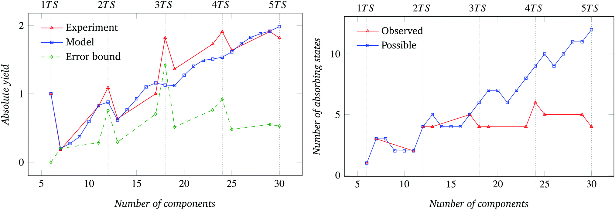
The results of the experiments are presented in Fig. 4–11 and in Fig. 17–20 of Appendix D. They show, in all cases, a qualitative agreement respectively with model-based predictions of absolute assembly yield Y, defined as the mean number of fully formed target structures over a given number of trials, and relative assembly yield T ≡ Y·N/n, defined as the mean number of components that form target structures divided by the number n of available components. For the comparisons of absolute yield, Fig. 4–11 (left) also report the 95% confidence error bound, i.e., the 95% confidence maximum difference between the predicted and the experimental absolute yields. Statistically significant confidence intervals were computed by means of the bootstrapping procedure described in Appendix B. A complementary measure of waste W, capturing the relative fraction of components not used in complete target structures, is defined as W ≡ 1 − Y·N/n = 1 − T and reported in Fig. 6 for the N = 8 case.

Circular sector components

As shown in Fig. 4, the yield in both the physical system and the abstract model is 100% for the 8-component condition. This is expected, since in this condition 8 components necessarily assemble in only one way if correctly placed and constrained to move in 2D (Fig. 5). Then, Y drops sharply for the 9-component condition, the first where the formation of incompatible substructures is possible. In fact, the 9-component system can end in one of 4 possible absorbing states (Fig. 5), three of which consist of two incompatible substructures. The values of the error bound, expectedly null for the n = 8 condition, show a non-monotonic increasing trend (Fig. 4).** The relative assembly yield also drops sharply for the 9-component condition, and initially shows a non-monotonic trend that becomes approximately constant at ∼31% for larger n (Fig. 17). Correspondingly, the component waste fraction W in Fig. 6 appears to converge asymptotically and non-monotonically to an approximately constant value of ∼69%.

Fig. 4 Results for the systems with N = 8 (45°) sectors per circular target structure: absolute assembly yield for experiments with physical system, absolute assembly yield for analytical model, and 95% error bound. Vertical dotted lines extend the markers on the x-axis for the fully formed target structures. Experimental data collected over 20 trials per condition.

Fig. 5 Number of possible and of observed absorbing states as a function of the number of components for the system of Fig. 4.

Fig. 6 Waste, i.e., relative fraction of components not assembled into target structures, for the system of Fig. 4.

The relation between absolute assembly yield and possible number of absorbing states is explicited in Fig. 16 of Appendix C. The curve is multi-valued since, as shown by Fig. 5, different values of n give rise to the same number of possible absorbing states. Nevertheless, a non-monotonic increase of Y with the number of possible states can generically be observed.

The absolute assembly yield data and error bounds for the 60°, 72°, and 90° sector conditions (Fig. 7–9 (left)) show non-monotonically increasing trends similar to the 45° sector case. The corresponding comparison between possible and observed absorbing states are shown in Fig. 7–9 (right). The relative yield data, presented in Fig. 17–20 of Appendix D, show the convergence of T to an N-dependent asymptotic value already observed for N = 8.

Fig. 7 Results for the systems with N = 6 (60°) sectors per circular target structure: (left) absolute assembly yield for experiments with physical system, absolute assembly yield for analytical model, and 95% error bound. Vertical dotted lines extend the markers on the x-axis for the fully formed target structures. Experimental data collected over 11 trials per condition. (right) Number of possible and of observed absorbing states as a function of the number of components.

Fig. 8 Results for the systems with N = 5 (72°) sectors per circular target structure: (left) absolute assembly yield for experiments with physical system, absolute assembly yield for analytical model, and 95% error bound. Vertical dotted lines extend the markers on the x-axis for the fully formed target structures. Experimental data collected over 11 trials per condition. (right) Number of possible and of observed absorbing states as a function of the number of components.

Fig. 9 Results for systems with N = 4 (90°) sectors per circular target structure: (left) absolute assembly yield for experiments with physical system, absolute assembly yield for analytical model, and 95% error bound. Vertical dotted lines extend the markers on the x-axis for the fully formed target structures. Experimental data collected over 11 trials per condition. (right) Number of possible and of observed absorbing states a function of the number of components.

Square and triangular components

The absolute assembly yield curve derived from the CRN-based model for the square components (Fig. 10 (left)) exactly matches that of the 90° sector components (Fig. 9 (left)). The match is expected, since the model parameters describing both component shapes—namely, bonding probability P^b and collision probability P^c—are the same (see Section 4). For the same reason, the number of possible absorbing states is also the same in both cases (Fig. 9 and 10 (right)). The data for relative assembly yield shown in Fig. 21 are consistent with previous observations.

Fig. 10 Results for systems with N = 4 (square-shaped) components per square target structure: (left) absolute assembly yield for experiments with physical system, absolute assembly yield for analytical model, and 95% error bound. Vertical dotted lines extend the markers on the x-axis for the fully formed target structures. Experimental data collected over 11 trials per condition. (right) Number of possible and of observed absorbing states a function of the number of components.

Yield data and number of absorbing states for systems of triangular components are shown in Fig. 11 (left), Fig. 22 and Fig. 11 (right), respectively. Also in this case, the absolute yield curves for experimental and model-based results have closely matching, non-monotonically increasing trends; not all possible absorbing states were observed; and T appears to saturate for large n.

Fig. 11 Results for systems with N = 3 (triangle-shaped) components per triangular target structure: (left) absolute assembly yield for experiments with physical system, absolute assembly yield for analytical model, and 95% error bound. Vertical dotted lines extend the markers on the x-axis for the fully formed target structures. Experimental data collected over 11 trials per condition. (right) Number of possible and of observed absorbing states as a function of the number of components.

Though time is not a parameter of our experiments, it is worth noting that the trials with the triangular components took 15 minutes on average to reach the absorbing state, compared to an average of 5 minutes for square- and sector-shaped components. This can be only partially justified by the use of a lower shaking frequency in the former case (see Section 5). Visual observations suggested that the triangular components tended to mutually align and stack themselves against the edge of the container. This ordering and packing effect induced by local component density³⁶ sterically hindered the roto-translational motion of the components and significantly reduced the rate of interbond formation.

Discussion

Experimental and analytical assembly yield data (Fig. 4, and (Fig. 7–11 (left))) show non-monotonically increasing, closely matching trends. Predicted and observed drops in assembly yield for specific n values can be justified by (1) the formation of the (z − 1)th target structure, and (2) the number of possible absorbing states.

Formation of the (z − 1)th target structure

Consider the experiment with 16 of the 45° circular sector components, which can form z = 2 target structures. If and when the first target structure is formed, the second target structure will also and always form. This is true since the residual components can assemble in only one way. This also implies that the probability of forming exactly one target structure is 0 in this condition. With one more component with respect to the previous condition, the second target structure is not guaranteed to form even if the first target structure is formed. This is true because the residual components could still form incompatible substructures. The expected drop in yield for the latter compared to the former condition was confirmed by the experimental data.

Beyond the third target structure, the formation of the (z − 1)th target structure does not seem to cause a significant drop in yield.

Number of possible absorbing states

The assembly yield is also influenced by the number of absorbing states a system can access (see Fig. 16) and the corresponding distribution of substructures. The number of possible absorbing states can be exactly computed for every set of components used in this work. Interestingly, for the conditions we studied, the number of possible absorbing states is not a monotonic function of the number of components in the system. This affects the assembly yield of the corresponding systems.

To improve the reliability of the experimental data, the absorbing state space of each assembly system should be completely explored, and a sufficient number of trials conducted to build a reliable empirical estimate of the distribution over the absorbing states.³⁷ Even with the non-negligible number of experimental trials we conducted (see Section 5), ultimately limited by time constraints, we were able to explore only a subspace of the possible absorbing states for all experimental conditions. In the experiment with N = 8 we did increase the number of trials per condition from 20 to 41 for selected values of n, as evidenced in Fig. 15. The additional trials did marginally help explore more of the absorbing state space (Fig. 5).

7 Scaling

Having verified the capability of the CRN-based model to predict the outcome of assembly experiments, we can use the model to investigate further properties of assembling systems of interest. Here, we begin by numerically exploring the scaling of the number of absorbing states and of assembly yield for populations of relatively large numbers of homogeneous components. Such conditions can be of significant practical interest in large-scale manufacturing (see Introduction).

The parallel and combinatorial nature of the assembly process and the existence of incompatible substructures let expect the number of absorbing states to be a power law function of the number of components. Fig. 12 plots the growth of the number of possible absorbing states with the number of components. It can be observed that different sets of components are associated with different scaling exponents; and that, in spite of the different geometry, pairs of sector-shaped components give rise to the same scaling exponent, respectively 1.00 in the case of 120° and 90° sector components and 1.92 for 72° and 60° ones. The origin of such subdivision remains to be investigated. A power law scaling of the absolute assembly yield with the number of components is derived from Fig. 13. In this case, all component types share a very similar scaling exponent (∼1.00). Scaling of the relative assembly yield with the number of components is shown in Fig. 14, which further evidences the convergence of T toward a fixed, N-dependent values for large values of n.

Fig. 12 Scaling of the number of possible absorbing states for large populations of homogeneous sector-shaped components of varying anisotropy.

Fig. 13 Scaling of absolute assembly yield for large populations of homogeneous sector-shaped components of varying anisotropy.

Fig. 14 Scaling of relative assembly yield for large populations of homogeneous sector-shaped components of varying anisotropy.

8 Conclusions

We presented a comprehensive study of assembly yield in systems of passive homogeneous agents assembling into equal target structures in parallel. The yield predictions derived from a chemical reaction network-based model were quantitatively compared with physical experiments conducted on a magneto-mechanical system. Our results demonstrate that the CRN-based model is able to predict with fair accuracy the assembly yield for the extensive presented set of experimental conditions parameterised by number and shape of components. The results provide a quantitative grounding as well as a generalisation of the incomplete evidence first reported by Hosokawa et al.²⁷ They evidence that the relative assembly yield for a given target structure tends to converge to a fixed value for populations with large number of components. Correspondingly, the average fraction of components ultimately not used in the assembly of complete target structures was shown to remain rather high (e.g., above 69% for the N = 8 case) irrespective of the number of components available, which posits severe waste concerns for practical applications. Our results also support the theoretical observation by Miyashita et al.,³⁰ according to which assembly yield increases as the angle of the sector-shaped components increases (i.e., N decreases). The CRN-based analysis clearly pinpointed the crucial role of incompatible substructures in the suboptimal yield in parallel assembly of geometrically-closed target structures, and was shown suitable to derive scaling laws for the assembly system. A similar analysis can be developed to model the 3D assembly of modular target structures—as reported e.g. by White et al.,³⁸ Hacohen et al.³⁴ and Neubert et al.³⁹—provided that CRNs and bonding probabilities are appropriately defined.

This work preludes to future analyses of ways to avoid incompatible substructures. A trivial solution to the problem is the compartmentalisation of the assembly space in subregions, each bounding the exact number of components making up a target structure. An obvious approach is also to convert the assembling system into a self-assembling system, whereby intercomponent bonds are reversible and can be broken under specific conditions.²⁴ In a system designed so that only the target structures do not break up upon collisions, the components population would be able to escape local energy minima. Another approach consists in templating the assembly of the target structures, for instance by using (non-homogeneous) sets of geometrically complementary components¹⁶ or addressable, uniquely-encoded intercomponent bonds.^34,40,41 In yet another approach, originally proposed but never realised by Hosokawa et al.,²⁷ mechanical conformational switching⁴² would direct the assembly kinetics of passive components with binary internal states and limit the number of possible coexisting nucleation sites.²⁰

Finally, the abstract model we used takes into account the combinatorial entropy of the system and a limited information on the geometry of the components. Additional entropic considerations might improve the model by integrating complementary spatial information pertaining to, e.g., component density in the assembly space.^7,36 Developing a model that takes into account spatial entropy will be part of our forthcoming work.

Conflicts of interest

There are no conflicts to declare.

Appendix A: CRN model for the N = 8 circular sector system

According to eqn (2), the F_i can then be expressed as:

Appendix B: Calculation of error bounds

Since gathering experimental data sufficient to compute 95% confidence intervals (CI 95%) is extremely time consuming for our assembling systems, we recurred to bootstrapping.³⁷ In this method, several independent samples are repeatedly drawn (with replacement) from an observed population in order to infer statistical information about the underlying distribution. The required statistics are computed for each independent sample, and a corresponding resampled distribution is built. As the observed population is assumed to contain all the necessary information of the underlying distribution, the resampled distribution represents the spread of the required statistic for the underlying distribution.³⁷

In our study, we bootstrap the physical experiment outcomes in order to obtain a confidence interval for the mean yield (μ_Y) of the physical experiments. Using the obtained confidence interval, the error bound, i.e., maximum difference between the model prediction and experimental mean, is calculated according to Algorithm 2. The experimental results (experimentalResults) are in the form of a matrix with numOfConditions rows and numOfTrials columns. We iterate through all the experiment conditions using the index i. A vector (μ_Y) of null values is initialised; this vector stores the yield values of the resampled data. For each condition, represented as a row in experimentalResults, we randomly choose (with replacement, i.e., resampled) values numOfTrials times. The yield of the resampled data is computed and stored in μ_Y. The process of resampling is repeated a given number of times (numOfBootstrapSamples).

The vector μ_Y is sorted in ascending order. As numOfBootstrapSamples = 200 in our work, the lower bound (lowerBound) is the 6th element, and the upper bound (upperBound) is the 195th element respectively. The error bound is the maximum difference between the model yield and one of the bounds.

The code and data employed to estimate the confidence intervals are available to download.††

Appendix C: Additional data for the assembly system with N = 8

For the case of target structures formed by 8 sector-shaped components, we hereby report the comparison of absolute assembly yield data and the 95% error bounds computed out of 20 and 41 trials (Fig. 15), and the relationship between absolute experimental assembly yield (for 20 trials) and number of possible absorbing states (Fig. 16).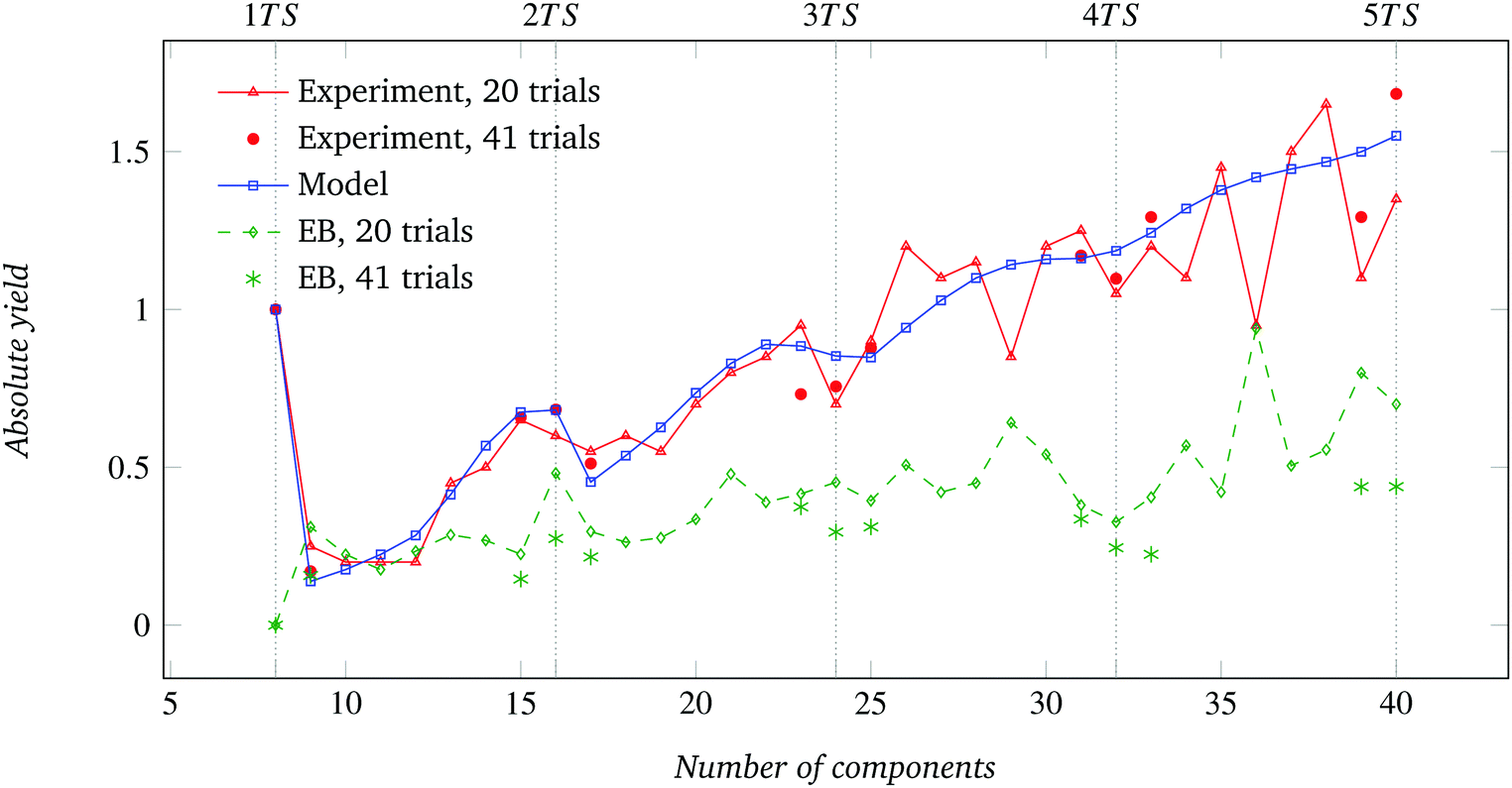

Fig. 15 Results for the systems with N = 8 (45°) sectors per circular target structure: comparison of model-predicted and experimental absolute assembly yield, including error bounds for 20 and 41 trials. Vertical dotted lines extend the markers on the x-axis for the fully formed target structures. See also Fig. 4.

Fig. 16 Scatter plot of absolute assembly yield as a function of possible absorbing states for the system with N = 8 (45°) sectors per circular target structure. Experimental yield values are from 20 trials (refer to Fig. 4 and 5).

Appendix D: Relative assembly yield

The plots of the relative assembly yield T = Y·N/n for the sector-, square- and triangle-shaped components are given in Fig. 17–22. Unless specified otherwise, 20 trials were performed for each experiment condition.

Fig. 17 Relative assembly yield for the system of Fig. 4 (N = 8).

Fig. 18 Relative assembly yield for the system of Fig. 7 (N = 6).

Fig. 19 Relative assembly yield for the system of Fig. 8 (N = 5).

Fig. 20 Relative assembly yield for the system of Fig. 9 (N = 4, sector-shaped components).

Fig. 21 Relative assembly yield for the system of Fig. 10 (N = 4, square-shaped components).

Fig. 22 Relative assembly yield for the system of Fig. 11 (N = 3, triangle-shaped components).

Acknowledgements

The work presented in this paper received funding from the European Research Council under the European Union Seventh Framework Programme (FP7/2007-2013)/ERC grant agreement no. 246939. Additionally, the authors would like to express their gratitude to: Joel Minsky for assisting in the fabrication of the components; Dr. Paolo Malgaretti for useful criticism and suggestions; Prof. Mauro Birattari, Alberto Franzin, Prof. Thomas Stützle, and Prof. Tom Wenseleers for giving critical insight into our data; and the Direct Manufacturing Research Center at the University of Paderborn for 3D printing the components used in the initial experiments.

References

1. C. J. Morris, S. A. Stauth and B. A. Parviz, IEEE Trans. Adv. Packag., 2005, 28, 600–611.
2. M. Mastrangeli, Q. Zhou, V. Sariola and P. Lambert, Soft Matter, 2017, 13, 304–327.
3. B. Grzybowski, C. E. Wilmer, J. Kim, K. P. Browne and K. J. M. Bishop, Soft Matter, 2009, 5, 1110–1128.
4. G. R. Desiraju, Crystal engineering: the design of organic solids, Elsevier, 1989.
5. A. J. Olson, Y. H. E. Hu and E. Keinan, Proc. Natl. Acad. Sci. U. S. A., 2007, 104, 20731–20736.
6. J. Madge and M. A. Miller, J. Chem. Phys., 2015, 143, 044905.
7. F. A. Escobedo, Soft Matter, 2014, 10, 8388–8400.
8. T. Hogg, Nanotechnology, 1999, 10, 300–307.
9. G. M. Whitesides and M. Boncheva, Proc. Natl. Acad. Sci. U. S. A., 2002, 99, 4769–4774.
10. G. M. Whitesides and B. Grzybowski, Science, 2002, 295, 2418–2421.
11. T. A. Witten Jr. and L. M. Sander, Phys. Rev. Lett., 1981, 47, 1400–1403.
12. A. Murugan, J. Zou and M. P. Brenner, Nat. Commun., 2015, 6, 6203.
13. W. Zheng and H. Jacobs, Adv. Funct. Mater., 2005, 15, 732–738.
14. L. Jacot-Descombes, C. Martin-Olmos, M. R. Gullo, V. J. Cadarso, G. Mermoud, L. G. Villanueva, M. Mastrangeli, A. Martinoli and J. Brugger, Soft Matter, 2013, 9, 9931–9938.
15. M. Mastrangeli, L. Jacot-Descombes, M. R. Gullo and J. Brugger, Proc. 2014 IEEE 27th International Conference on Micro Electro Mechanical Systems (MEMS), 2014, pp. 56–59.
16. N. Bhalla, D. Ipparthi, E. Klemp and M. Dorigo, Parallel Problem Solving from Nature XIII, Springer, 2014, pp. 751–760.
17. G. M. Whitesides, J. P. Mathias and C. Seto, Science, 1991, 254, 1312–1319.
18. K. E. Schwiebert, D. N. Chin, J. C. MacDonald and G. M. Whitesides, J. Am. Chem. Soc., 1996, 118, 4018–4029.
19. B. Alberts, D. Bray, J. Lewis, M. Raff, K. Roberts and J. D. Watson, Molecular biology of the cell, Garland Publishing, Inc., 1994.
20. R. P. Sear, J. Phys.: Condens. Matter, 2007, 19, 033101.
21. L. S. Penrose and R. Penrose, Nature, 1957, 179, 1183.
22. N. Bowden, I. S. Choi, B. A. Grzybowski and G. M. Whitesides, J. Am. Chem. Soc., 1999, 121, 5373–5391.
23. D. H. Gracias, J. Tien, T. L. Breen, C. Hsu and G. M. Whitesides, Science, 2000, 289, 1170–1172.
24. F. Ilievski, M. Mani, G. M. Whitesides and M. P. Brenner, Phys. Rev. E: Stat., Nonlinear, Soft Matter Phys., 2011, 83, 017301.
25. R. Cademartiri, C. A. Stan, V. M. Tran, E. Wu, L. Friar, D. Vulis, L. W. Clark, S. Tricard and G. M. Whitesides, Soft Matter, 2012, 8, 9771–9791.
26. M. Grünwald, S. Tricard, G. M. Whitesides and P. L. Geissler, Soft Matter, 2016, 12, 1517–1524.
27. K. Hosokawa, I. Shimoyama and H. Miura, Artif. Life, 1994, 1, 413–427.
28. E. Klavins, IEEE Contr. Syst. Mag., 2007, 27, 43–56.
29. B. Haghighat and A. Martinoli, Swarm Intell., 2017, 11 DOI:10.1007/s11721-017-0139-4.
30. S. Miyashita, M. Göldi and R. Pfeifer, Int. J. Rob. Res., 2011, 30, 627–641.
31. G. Mermoud, M. Mastrangeli, U. Upadhyay and A. Martinoli, Proc. 2012 IEEE International Conference on Robotics and Automation (ICRA), 2012, pp. 4266–4273.
32. B. Haghighat, M. Mastrangeli, G. Mermoud, F. Schill and A. Martinoli, Micromachines, 2016, 7, 138.
33. M. Mastrangeli, F. Schill, J. Goldowsky, H. Knapp, J. Brugger and A. Martinoli, Proc. 2014 IEEE International Conference on Robotics and Automation (ICRA), 2014, pp. 5860–5865.
34. A. Hacohen, I. Hanniel, Y. Nikulshin, S. Wolfus, A. Abu-Horowitz and I. Bachelet, Sci. Rep., 2015, 5, 12257.
35. D. T. Gillespie, Annu. Rev. Phys. Chem., 2007, 58, 35–55.
36. D. Frenkel, Nat. Mater., 2015, 14, 9–12.
37. B. Efron and R. J. Tibshirani, An introduction to the bootstrap, CRC Press, 1994.
38. P. White, V. Zykov, J. C. Bongard and H. Lipson, Robotics: Science and Systems, 2005, pp. 161–168.
39. J. Neubert, A. P. Cantwell, S. Constantin, M. Kalontarov, D. Erickson and H. Lipson, IEEE International Conference on Robotics and Automation (ICRA), 2010, pp. 2479–2484.
40. W. M. Jacobs, A. Reinhardt and D. Frenkel, Proc. Natl. Acad. Sci. U. S. A., 2015, 112, 6313–6318.
41. D. Ipparthi, M. Mastrangeli and A. Winslow, Theor. Comput. Sci., 2017, 671, 19–25.
42. K. Saitou, IEEE Trans. Rob. Autom., 1999, 15, 510–520.

---

Footnotes

† Current address: College of Engineering and Computer Science, The University of Texas Rio Grande Valley, Edinburg, USA.

‡ Current address: Department of Microelectronics, Delft University of Technology, Delft, The Netherlands. E-mail: m.mastrangeli@tudelft.nl

§ The parallel assembly of target structures composed of pairs of components is not affected by incompatible substructures, since in this case the only substructures are single components, and there is a single absorbing state associated to each number of components. This limit case has important technological applications, such as, e.g., the sequential three-dimensional self-assembly and packaging of light emitting diodes¹³ and the self-assembly of polymeric microcapsules.^14,15

¶ N = 8 represents a more complex case than the N = 6 case presented by Hosokawa et al.,²⁷ Miyashita et al.³⁰ and Klavins.²⁸ In our experiments, N was limited to 8 by fabrication constraints.

|| A sample video of an assembly trial is available at http://iridia.ulb.ac.be/~dipparth/site/video/.

** When computing the yield considering also the additional 21 trials (i.e., on a total of 41 trials), the difference between the model prediction and the observed value becomes smaller; similarly, the corresponding bounds are reduced (see Fig. 15 in Appendix C).

†† http://iridia.ulb.ac.be/~dipparth/site/.

---