Performance evaluation of gasoline alternatives using a thermodynamic spark-ignition engine model†
Received
2nd June 2017
, Accepted 28th August 2017
First published on 29th August 2017
Abstract
In light of climate change and due to the fact that surface transportation heavily relies on internal combustion engines, many different alternatives to gasoline have been proposed. Herein, we present a model, incorporating only first order effects, which allows a quick assessment of the suitability of a certain molecule as a replacement for gasoline. Using global sensitivity analysis, the elemental composition and the vapor heat capacity have been identified as main influencing fuel parameters. A case study using the currently proposed alternative fuels (methanol, ethanol, n-butanol, dimethylfuran, methylfuran, and α-pinene) as well as gasoline and several hydrocarbons (cyclohexane, n-heptane, isooctane, and benzene) revealed n-butanol as the best performing alternative fuel. The use of this compound entails a significant decrease in CO2 emissions and an increased efficiency, but also a higher consumption in comparison with gasoline.
1 Introduction
Upon analysis of the worldwide CO2 emissions, it becomes evident that transportation is the second largest contributor, following electricity and heat generation.1 To reduce CO2 emissions from electricity and heat generation, a series of technologies have already been developed, such as hydro-, solar- or wind power stations. For transportation, however, the situation is different. Although several concepts have been proposed, ranging from alternative fuels to different means of propulsion, the discussion is still ongoing.2 Alternatives to the Internal Combustion Engine (ICE) as well as the selection of alternative fuels for ICE are discussed.3,4
It is estimated that the ICE will remain dominant in surface transportation with a share above 80% by 2030.5 This implies the need for renewable fuels in order to reduce global CO2 emissions significantly.
Currently, the most commonly used alternative fuel for Spark Ignition (SI) engines is ethanol. Other compounds that are frequently discussed include methanol, n-butanol, and more recently 2-methylfuran (MF) and 2,5-dimethylfuran (DMF).6,7 Recently, Raman et al.8 proposed the use of α-pinene as a gasoline replacement because its energy content is similar to gasoline and therefore a similar range is expected. The different production pathways and the discussion of non-engine related properties can be found in the literature.9,10 Within this study, these compounds as well as representatives of all gasoline compound classes (n-heptane for straight chain hydrocarbons, iso-octane for branched hydrocarbons, cyclohexane for cyclic hydrocarbons, and benzene for aromatic compounds) were investigated. Methyl tert-butyl ether (MTBE) serves as a further example for oxygenated compounds.
Bypassing petroleum-based routes will affect all processes and technologies involved in producing, refining, upgrading and using these fuels. One major concern, for instance, is the higher oxygen and nitrogen concentrations in biomass feedstocks. Thus, elaborate processes for denitrogenation and deoxygenation have to be applied to minimize the oxygen and nitrogen concentrations in the fuel. The presence of oxygen reduces the Lower Heating Value (LHV) of the fuel and thereby the energy content of a given volume of fuel. Fuel-bound nitrogen is either converted into NOx or N2, depending mainly on the molecular structure. Regardless of this, the presence of both elements affects the pathway and the rate of combustion.
Plenty of studies have been conducted experimentally as well as theoretically to assess the performance of different fuels. The comparison of two different experimental studies is often hindered by the variable degrees of freedom in the load, the engine and the testing procedure. One way to overcome this problem is to utilize gasoline as a benchmark.11,12 This approach requires knowledge of the influence of each property, complicating quantitative statements. Simulation tools ranging from 0D thermodynamic approaches to 3D Computational Fluid Dynamics (CFD) codes might be another solution. The strength of CFD codes lies within the detailed representation of the thermal and fluidic processes within the engine. They are mainly used for engine design purposes. Meanwhile, 0D thermodynamic models are built primarily for their fast rather than accurate analysis and are, therefore, ideal for the comparison of different fuels. Several approaches have been reported in the literature: a model comparing hydrogen, propane, methane and methanol has been presented13 using 1D modelling. The combustion part was defined separately, based on experimental correlations for each fuel. Another model focused on emissions and gas dynamic effects.14 The processes within the engine were studied by using a spark ignition engine model using pressure traces obtained empirically.15 Shen et al.16 published a model to predict the pressure trace during methanol combustion. Ramachandran17 proposed a fast model including detailed chemical reactions. The model lacks, however, the ability to detect knocking, neglects friction within the engine and is limited to the combustion engine itself. Mehrnoosh et al.18 presented a model for engines that run on gasoline and natural gas with a focus on NO emissions, the combustion rate and knocking.
The present contribution is based on a thermodynamic model of an SI ICE with special emphasis on the influence of the fuel. It involves an optimization of the compression ratio for each fuel such that the efficiency is maximized and knocking does not occur. The potential of the currently discussed liquid fuel molecules as gasoline replacements is addressed at a fundamental level from an engine perspective.
2 Thermodynamic engine model
The performance of different liquid fuels was evaluated by means of a thermodynamic model of an SI Direct Injection (DI) ICE running under stoichiometric conditions (air–fuel equivalence ratio, λ = 1). The performance was assessed with respect to the engine efficiency at different loads and for three driving cycles, including the specific CO2 emissions. Other emissions such as NOx, CO, or soot have not been modeled. All first-order influences on the performance linked to the fuel properties were considered. A detailed description of the modeling steps is given in Appendix A.
Besides the engine, the model includes the following auxiliary systems: a turbocharger powered by an exhaust gas turbine, a fuel pump and an after-cooler.
2.1 Process description
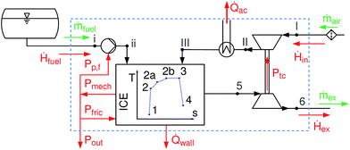
A schematic overview of the model is given in Fig. 1. The process starts with air under ambient conditions (I); the air is then compressed and cooled (III) before entering the cylinder. After the intake, compression starts (1 → 2); the combustion within the cylinder is modeled according to the T-s diagram approach,19 splitting the combustion into an isochoric (2 → 2a), an isobaric (2a → 2b) and an isothermal phase (2b → 3). Expansion of the burnt gases (3 → 4) and gas exhaust through the turbine (5, 6) complete the cycle. Frictional losses Pfric and wall heat losses ![[Q with combining dot above]](https://www.rsc.org/images/entities/i_char_0051_0307.gif) wall within the cylinder are accounted for. The model is limited to fuels that are liquid under ambient conditions.
wall within the cylinder are accounted for. The model is limited to fuels that are liquid under ambient conditions.
 |
| | Fig. 1 Flow sheet representation of all engine parts considered. System boundary as dashed blue line. Pp,f is the power supplied to the fuel pump, Ptc power transferred from the turbocharger turbine to the compressor, Pout the net power output of the engine, Pmech the mechanical power, Pfric the friction losses within the engine, ![[Q with combining dot above]](https://www.rsc.org/images/entities/i_char_0051_0307.gif) wall the wall heat losses, wall the wall heat losses, ![[Q with combining dot above]](https://www.rsc.org/images/entities/i_char_0051_0307.gif) ac the heat transferred by the after-cooler, and Ḣ, ṁ the enthalpy stream/massflow of intake, exhaust or fuel. ac the heat transferred by the after-cooler, and Ḣ, ṁ the enthalpy stream/massflow of intake, exhaust or fuel. | |
To obtain a meaningful comparison of the potential of different fuels, the compression ratio is optimized for each fuel. Accordingly, the model is split into two different parts: on the one hand, the engine model itself, and on the other hand, an optimization procedure to maximize the efficiency for each fuel and to avoid knocking. The adaptation of the engine to the fuel is done by changing the compression ratio (εCR ∈ [5, 20]), while the total cylinder volume (volume at the Bottom Dead Center (BDC)) is kept constant.
2.2 Input parameters and derived fuel properties
The investigated fuels are characterized by several parameters, summarized in Table 1. Please note that the bounds given in Table 1 only apply to the Sensitivity Analysis (SA). The input to the model is limited to compounds which are liquid at room temperature. The estimation of the LHV was done via the correlation for the Higher Heating Value (HHV) presented by Channiwala and Parikh,20 which leads to eqn (1).| | | LHV = 418.92x + 95.85y − 165.44z − 21.14v kJ mol−1 | (1) |
Table 1 List of fuel parameters (at 298 K and 0.1 MPa) and their bounds in the SA, (Section 4)
| Input factor |
|
Units |
Bounds in SA |
| Number of C atoms |
x
|
— |
[1, 11] |
| Number of H atoms |
y
|
— |
[0, 24] |
| Number of O atoms |
z
|
— |
[0, 11] |
| Number of N atoms |
v
|
— |
[0, 11] |
| Vapor heat capacity |
![[c with combining macron]](https://www.rsc.org/images/entities/i_char_0063_0304.gif) p,g
p,g
|
J kg−1 K−1 |
[1200, 2000] |
| Liquid heat capacity |
![[c with combining macron]](https://www.rsc.org/images/entities/i_char_0063_0304.gif) p,L
p,L
|
J kg−1 K−1 |
[1700, 3000] |
| Fuel density |
ρ
|
kg m−3 |
[500, 1500] |
| Liquid kinematic viscosity |
ν
|
m2 s−1 |
[2, 100] × 10−7 |
| Vapor pressure at 298 K |
p
vap
|
Pa |
[1.5, 100] × 103 |
| Enthalpy of vaporization |
![[h with combining macron]](https://www.rsc.org/images/entities/i_char_0068_0304.gif) vap
vap
|
J kg−1 |
[2, 12] × 105 |
| Research octane number |
RON |
— |
[50, 115] |
| Surface tension |
σ
|
N m−1 |
[0.01, 0.1] |
The vapor pressure (pvap) at the normal boiling point (Tboil) is by definition equal to the ambient pressure (pamb). The vapor pressure, the heat of vaporization (hvap) and the temperature (T) are related by the Clausius–Clapeyron equation. Under the assumption that the heat of vaporization is independent of the temperature, eqn (2) was derived:
| |  | (2) |
with the reference temperature (
Tref) at which
hvap and
pvap have been measured, the universal gas constant (
R).
2.3 Fuel injection and evaporation
At the start of the compression, the fuel is injected instantaneously and evaporates during the compression stroke. Any fuel which is not evaporated at the Top Dead Center (TDC) is considered to be incombustible. The initial droplet diameter is estimated based on the nozzle diameter of the fuel injector, initial droplet velocity, the Weber number and the Reynolds number. Droplet evaporation was modeled according to the d2-law as proposed by Godsave.21 Details can be found in Sections A.1.1 and A.1.2 of the Appendix.
2.4 Compression and expansion
The wall heat losses during compression and expansion were modeled using the correlation of Hohenberg.22 Its use for fuels other than gasoline is justified by an error estimation presented in Appendix B. By integrating the first law of thermodynamics, the conditions at the end of the process substep can be determined.
2.5 Combustion
As depicted schematically in Fig. 2, the combustion of the evaporated fuel was split into three sequential processes: firstly, isochoric combustion (2 → 2a); secondly, isobaric combustion (2a → 2b); and thirdly, isothermal combustion (2b → 3). It is assumed that the properties of the gas mixture in the cylinder depend linearly on the combustion progress.
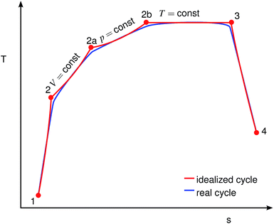 |
| | Fig. 2 Comparison of idealized and real engine cycles, adapted from ref. 19. Red: idealized cycle, blue: real cycle. | |
The total wall heat losses (Qw,tot,0) were approximated considering the Reynolds analogy for the heat flux of the established turbulent flows:
| |  | (3) |
with bore
B, charge pressure ratio
Πtc, the empirical constant
Kq,tot and the mean piston speed
cm (=2
SN) (stroke
S, rotational speed
N).
εtot is the total energy input of the yet unburnt mixture which is calculated based on the LHV, the number of fuel molecules (
nfuel) and total number of molecules within the un-/burnt (
nub/b) mixture as well as the enthalpies (
hub/b) of the un-/burnt mixtures at a reference temperature of 298 K.
| |  | (4) |
Inspired by the heat transfer correlation of Hohenberg,22 a dependence of the total wall heat losses on the peak pressure (ppeak) was introduced as follows:
| |  | (5) |
The dependence of the overall heat losses during combustion on the peak pressure leads to the need for an iterative solver as the peak pressure depends on the total heat losses. Therefore, the secant method23 is employed to find suitable solutions for the peak pressure and the respective heat loss.
The fundamental equations used to model the three phases of combustion are:
| | | cV,2aT2a − cV,2T2 = 0.66(εtot − Qw,tot) | (6) |
| | | cp,2bT2b − cp,2aT2a = 0.20(εtot − Qw,tot) | (7) |
| | | T3Δs3,2b + Δh3,2b = 0.14(εtot − Qw,tot) | (8) |
depending on the heat capacity at constant volume
cV and constant pressure
cp as well as the entropy difference Δ
s. The indices refer to the thermodynamic cycle in a T-s diagram, as shown in
Fig. 2. The values 0.66, 0.20, 0.14 are empirically deduced from fitting the overall efficiency of gasoline
vs. different loads and rotational speeds, based on measurements from our test bench. They lie well within the recommended ranges, 0.5 to 0.7, 0.1 to 0.3 and 0.1 to 0.2, respectively.
19 Although different fuels have different flame speeds which should implicate different fractions of the three combustion phases, it has been shown that for a well-controlled engine the combustion duration remains constant.
24 The reason is that for any given SI engine the engine control will adjust the ignition timing such that the main heat release occurs just after the TDC. To ensure the mechanical integrity of the engine, a peak pressure limitation also has to be introduced, imposing an upper limit on the fraction of the isochoric combustion phase. From an efficiency point of view, it is desirable to minimize the isothermal part. Since the heat capacities in
eqn (6) to (8) depend on the unknown temperatures at the end of the cycle step, the secant method is applied to solve them iteratively.
2.6 Knock model
Knocking denotes the phenomenon that during combustion parts of the unburnt mixture ignite before being reached by the flame front. It is generally estimated using the knock integral. Its value reaches 1 at the onset of knocking:| |  | (9) |
| |  | (10) |
The assumption of isochoric combustion from 2 → 2a leads to an infinitely short time span such that  . The ignition delay (τig) is approximated by using the correlation proposed by Douaud and Eyzat.25
| |  | (11) |
where
p and
Tub are the pressure and the temperature of the unburnt mixture. To obtain these values the unburnt zone needs to be introduced, leading to a quasi 2-zone model. The following assumptions are made: firstly, the pressures of the burnt and the unburnt gases are equal, and secondly, the temperature of the unburnt mixture (
Tub) is calculated following an isentropic process starting just before combustion:
| |  | (12) |
with the heat capacity ratio (
γ) of the unburnt mixture.
2.7 Friction
Several friction models were evaluated. The friction model of Chen and Flynn26 was chosen due to its simplicity, in terms of input parameters, and consideration of the peak pressure (ppeak) as well as the mean piston speed (cm). This model allows accurate calculation of the friction mean effective pressure (fmep).| | | fmep = fmep0 + β0ppeak + β1cm + β2cm2 | (13) |
The empirical constants β0,…,2 and fmep0 are deduced from a fit to data measured on our test bench. Detailed information on the fit is given in Appendix C.
2.8 Gas exchange
As a first approximation, the low pressure cycle is modeled using two pressure levels (both are assumed to be constant). The first level is the intake pressure (p1) which is defined by the charge pressure provided by the compressor. The second level is defined by the back pressure (p4,bt) of the turbocharger turbine. The work needed by the compressor (Wc,needed) to deliver the desired charging can be described as follows:| |  | (14) |
where κin denotes the heat capacity ratio of air and Tamb is the ambient temperature. This leads to the following equation for the turbine back pressure:| | 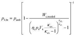 | (15) |
Finally, the power required (Pgas,ex) during the low pressure cycle can be described, in dependence of the displacement volume VD, the number of cylinders ncyl and the rotational speed N, as:
| |  | (16) |
The efficiencies of the turbine (ηt) and of the compressor (ηc) are 0.65 and 0.70, respectively.27 In order to model the throttle valve for part-load operation, the charge pressure ratio (Πtc) can be reduced below 1. Below this value the back pressure is fixed at 107.5 kPa, thereby accounting for pressure losses over the exhaust system. For modeling the decreased turbine efficiency at low rotational speeds of the turbine, the following assumptions were made. Firstly, above an engine rotational speed of 1500 rpm the maximum charge pressure ratio (Πtc) of 2 is achieved; secondly, at 1000 rpm the engine is run as an aspirated engine (Πtc = 1) and thirdly, at in-between rotational speeds the charge pressure ratio is linearly dependent on the rotational speed of the engine. The actual charge pressure ratio can then be chosen either as an input value or such that the required power output is met.
2.9 Model output
To judge the performance of a fuel, the following values are calculated based on the fuel properties, the engine parameters and the simulation results: the efficiency (η) at different loads and the specific CO2 emissions at full load (eCO2) in g kWh−1. The definitions are given in eqn (17) and (18).| |  | (17) |
| |  | (18) |
The results for full load (FL) are reported at 2000 rpm. Part load (PL) is defined as a power output of 6.6 kW at 2000 rpm, which is the power output of the gasoline engine at a brake mean effective pressure (bmep) of 2 bar.
2.10 Driving cycle modeling
Different car designs are compared by using standardized driving cycles. Within this paper, the worldwide harmonized light vehicles test cycle (WLTC),28 the Common Artemis Driving Cycle (CADC)29 and the New European Driving Cycle (NEDC)30 were investigated. To be able to predict the performance of a fuel, not only a model of the engine but of the whole vehicle is required. A comparison of different fuels is only meaningful as long as the vehicle remains the same. Therefore, the complexity of the vehicle model is reduced to the minimum. The total force acting upon the vehicle (Ftot) is calculated based on the velocity defined by the cycle, considering friction, drag and acceleration forces.31| |  | (19) |
The values of the constants are listed in Table 2. The gearbox is neglected and it is assumed that each point within the engine map can be reached. The whole drivetrain (without the engine) is assumed to have a mechanical transmission efficiency of ηtrans = 0.85. The power required from the engine Peng,req then becomes:
| |  | (20) |
Table 2 Constants of the vehicle model31
| Property |
Symbol |
Value |
| Gravitational acceleration |
g
|
9.81 m s−2 |
| Friction coefficient |
μ
|
0.0085 |
| Vehicle mass |
m
|
1500 kg |
| Drag coefficient |
c
D
|
0.3 |
| Front area |
A
|
2.2 m2 |
| Air density |
ρ
air
|
1.2 kg m−3 |
| Acceleration coefficient |
C
acc
|
1.05 |
The value of the acceleration coefficient (Cacc) is set to 1.05 in order to reflect the moment of inertia of all the rotating parts (wheels, flywheel, etc.). To provide a reasonable comparison between the different fuels, the cylinder volume is adjusted such that at 2000 rpm and full load the engine provides the same power output as the gasoline engine (71 kW). This is done by applying the secant method and keeping the bore to stroke ratio constant. The model is run as quasi-stationary simulation, thereby ruling out all the dynamic effects of switching gears and acceleration on the performance of the engine. For each required power value the efficiency is optimized by adjusting the rotational speed and the charge pressure under the boundary condition that the rotational speed of the engine may not be below 1000 rpm. For each load point (i) the fuel consumption (ṁF,i), power output (PF,i) and absolute CO2 emissions (eCO2,i) are determined.
The cycle efficiency (ηcyc), the CO2 emissions with respect to power (eCO2,P) and distance (eCO2,D) and the consumption (consumptioncyc) are defined as follows:
| |  | (21) |
| |  | (22) |
| |  | (23) |
| |  | (24) |
3 Investigated fuels
Besides gasoline, some gasoline components (iso-octane, n-heptane, cyclohexane and benzene), MTBE, a well-known gasoline additive, and several possible substitutes (methanol, ethanol, MF and DMF) were chosen for this study. The fuel properties are shown in Table 3. If not stated otherwise, their properties have been taken from the DIPPR database.32
Table 3 Fuel molecules and their properties under standard conditions (T = 298 K, p = 0.1 MPa) investigated within this study
| Fuel |
H:C [mol mol−1] |
O:C [mol mol−1] |
M [kg kmol−1] |
ρ [kg m−3] |
c
p,g [J mol−1 K−1] |
h
vap [kJ mol−1] |
p
vap [kPa] |
ν [mm2 s−1] |
RON [—] |
LHV [MJ mol−1] |
|
Methyl tert-butyl ether.
2-Methylfuran.
2,5-Dimethylfuran.
Estimated according to ref. 20.
By definition.
|
| Gasoline |
2.00![[thin space (1/6-em)]](https://www.rsc.org/images/entities/char_2009.gif) 33 33 |
0 |
98 |
748![[thin space (1/6-em)]](https://www.rsc.org/images/entities/char_2009.gif) 34 34 |
154.6![[thin space (1/6-em)]](https://www.rsc.org/images/entities/char_2009.gif) 35 35 |
34.5![[thin space (1/6-em)]](https://www.rsc.org/images/entities/char_2009.gif) 36 36 |
34.3![[thin space (1/6-em)]](https://www.rsc.org/images/entities/char_2009.gif) 33 33 |
0.41![[thin space (1/6-em)]](https://www.rsc.org/images/entities/char_2009.gif) 36 36 |
98e |
4.27d |
| Iso-octane |
2.25 |
0 |
114 |
689 |
187.1 |
35.2 |
6.5 |
0.69 |
100e |
5.08d |
|
n-Heptane |
2.29 |
0 |
100 |
680 |
164.3 |
36.6 |
6.0 |
0.58 |
0e |
4.47d |
| Cyclohexane |
2.00 |
0 |
84 |
772 |
107.0 |
32.9 |
13.0 |
1.16 |
83![[thin space (1/6-em)]](https://www.rsc.org/images/entities/char_2009.gif) 37 37 |
3.66d |
| Benzene |
1.00 |
0 |
78 |
872 |
82.7 |
33.9 |
12.6 |
0.69 |
108![[thin space (1/6-em)]](https://www.rsc.org/images/entities/char_2009.gif) 38 38 |
3.09d |
| MTBEa |
2.40 |
0.20 |
88 |
735 |
135.3 |
30.1 |
33.1 |
0.46 |
117![[thin space (1/6-em)]](https://www.rsc.org/images/entities/char_2009.gif) 39 39 |
3.08d |
| Methanol |
4.00 |
1.00 |
32 |
789 |
44.0 |
37.5 |
16.7 |
0.68 |
109![[thin space (1/6-em)]](https://www.rsc.org/images/entities/char_2009.gif) 40 40 |
0.64d |
| Ethanol |
3.00 |
0.50 |
46 |
785 |
65.1 |
42.6 |
7.9 |
1.38 |
109![[thin space (1/6-em)]](https://www.rsc.org/images/entities/char_2009.gif) 36 36 |
1.25d |
|
n-Butanol |
2.50 |
0.25 |
74 |
805 |
110.0 |
52.5 |
0.9 |
3.53 |
98![[thin space (1/6-em)]](https://www.rsc.org/images/entities/char_2009.gif) 36 36 |
2.47d |
| MFb |
1.20 |
0.20 |
82 |
913![[thin space (1/6-em)]](https://www.rsc.org/images/entities/char_2009.gif) 36 36 |
89.6![[thin space (1/6-em)]](https://www.rsc.org/images/entities/char_2009.gif) 41 41 |
29.4![[thin space (1/6-em)]](https://www.rsc.org/images/entities/char_2009.gif) 41 41 |
18.5![[thin space (1/6-em)]](https://www.rsc.org/images/entities/char_2009.gif) 41 41 |
4.00![[thin space (1/6-em)]](https://www.rsc.org/images/entities/char_2009.gif) 42 42 |
103![[thin space (1/6-em)]](https://www.rsc.org/images/entities/char_2009.gif) 36 36 |
2.50d |
| DMFc |
1.33 |
0.17 |
96 |
889![[thin space (1/6-em)]](https://www.rsc.org/images/entities/char_2009.gif) 43 43 |
135.4![[thin space (1/6-em)]](https://www.rsc.org/images/entities/char_2009.gif) 41 41 |
32.0![[thin space (1/6-em)]](https://www.rsc.org/images/entities/char_2009.gif) 41 41 |
7.1![[thin space (1/6-em)]](https://www.rsc.org/images/entities/char_2009.gif) 41 41 |
0.65![[thin space (1/6-em)]](https://www.rsc.org/images/entities/char_2009.gif) 44 44 |
119![[thin space (1/6-em)]](https://www.rsc.org/images/entities/char_2009.gif) 36 36 |
3.12d |
| α-Pinene |
1.60 |
0 |
136 |
858![[thin space (1/6-em)]](https://www.rsc.org/images/entities/char_2009.gif) 8 8 |
172.9 |
35.6![[thin space (1/6-em)]](https://www.rsc.org/images/entities/char_2009.gif) 8 8 |
6.4![[thin space (1/6-em)]](https://www.rsc.org/images/entities/char_2009.gif) 8 8 |
1.74 |
85![[thin space (1/6-em)]](https://www.rsc.org/images/entities/char_2009.gif) 8 8 |
5.72d |
4 Sensitivity analysis
The developed engine model encompasses various parameters, correlations and equations that interact and affect the model output at the same time. In order to gain more insight into the model, Global Sensitivity Analysis (GSA) was performed to link the variation in the model output γ to the variation of the input factors χ. A popular GSA approach is the Elementary Effects (EEs) method that allows ranking/screening of input factors at low computational cost.45 The method is based on averaging locally calculated EEs around base points, distributed in the input factor hyperspace. Herein, EEij of the ith input factor χi for the jth base point Xj and the perturbation Δ is calculated as| |  | (25) |
Base points and perturbations were generated by using a Latin Hypercube (LH) approach.46,47 The mean EE  , averaged over n calculated EEs and its normalized form Si are measures of the total sensitivity of the ith of M input factors.48
| |  | (26) |
The performed SA investigated the effect of 12 input factors (see Table 1) on three model outputs, including ηFL, PFL and eCO2,FL. Bounds for input factors are listed in Table 1 and are based on the ranges of the parameters as given in Table 3, being representative of a wide choice of fuels. Sensitivity values were obtained after 4.8 × 10⁵ model evaluations (N = n(M + 1), see Fig. 10 for convergence).
5 Results & discussion
5.1 Experimental validation
The thermodynamic engine model is validated against experimental data of an SI ICE run on commercial gasoline (Research Octane Number (RON) 98) with a displacement of two liters which was operated under fully warmed-up conditions on an engine test bench. Table 8, in the Appendix, shows the main characteristics of the experimental setup. Validation is discussed here at an engine speed of 2000 rpm. Passenger car engines are frequently operated at a speed around 2000 rpm and the engines are typically optimised for good efficiency and good drivability in this speed region. Additionally, turbocharged engines typically achieve a peak torque around 2000 rpm and exhaust gas temperatures are not too high such that the engine can safely be operated at λ = 1. Boosted engines typically show clear knock tendencies at 2000 rpm and high load so that the knock model can also be validated at the considered speed.
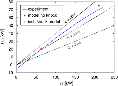
Fig. 3 shows a so-called Willans-type49 plot for 2000 rpm. This direct representation of input power versus output power is a meaningful approach for the analysis of energy conversion devices at different loads.49–51 Here, the input power is calculated as:
and output power is the power at the engine's flywheel.
Fig. 3 shows that the measured input–output correlation is linear until approximately 50 kW output power (this corresponds to approximately 17 bar bmep). At higher loads, the curve bends towards lower efficiencies. The reason is that the ignition has to be delayed in this load regime to avoid knock. The model was used to simulate the operating points 2 bar bmep, 6 bar bmep and full load.
Fig. 3 shows that the model simulation meets the measured efficiencies very well for the two part-load points. For the full load point, the output power and efficiency are overestimated by the model, if knock is not taken into account. However, the model correctly detects knocking under these conditions making it clear that this output power cannot be achieved in reality without adjusting the ignition timing. The reaction of the model is to decrease the compression ratio
εCR as described in Appendix A.2. In this particular case, the model reduced
εCR from 10 to 7.7. The corresponding result is also plotted in
Fig. 3. Upon reducing
εCR, the power output declines, matching the measured level. Again, no model parameter was adjusted to the measured data to obtain this match. Thus,
εCR reduction shows a similar effect on the power output and efficiency as the ignition timing postponement of the real engine.
 |
| | Fig. 3 Input–output power characteristics for gasoline operation at 2000 rpm, the measured engine results versus the model results. Blue line: experiment, red squares: the modeling results without knock detection (the same compression ratio as in the experiments), cyan diamond: the modeling result with the adapted compression ratio to avoid knock, black dotted lines: lines of constant efficiency. | |
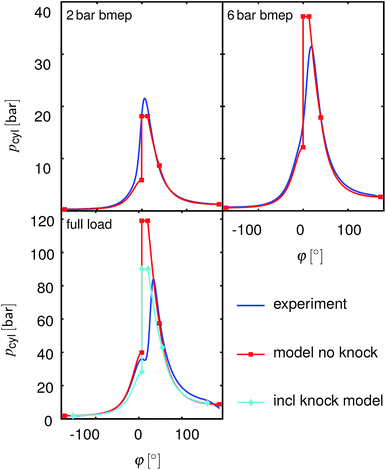
As described in Section 2.5, the model calculates heat release as an isochoric process at the Top Dead Center (TDC), followed by an isobaric process and an isothermal process with constant shares of these phases for all operating points. Fig. 4 shows the measured and simulated pressure traces for the operating points shown in Section 3. The simulation approximates the real behavior well at the 2 bar bmep operating point; the deviation is larger for the two other operating points considered. However, the differences appear mainly close to the TDC where the volume change is small and thus the error in bmep (or Pout) is also small.
 |
| | Fig. 4 Measured and simulated pressure traces at N = 2000 rpm and different loads for gasoline operation. Blue: measurements, red: the modeling results without knock detection, cyan: modelling results with adapted compression ratio to avoid knock. phi: crank angle. | |
In conclusion, the model is able to reproduce the experimental efficiency and output power results for gasoline operation across a wide range of engine loads. Other fuels could not be experimentally tested as the engine's fuel system is not compatible with alternative fuels. The validity of the model for alternative fuels is critically discussed in the following sections.
5.2 Extended validation
Using experimental data from a Spark Ignition Internal Combustion Engine run on gasoline, the model is able to predict the performance of such an engine. The application of the model to fuels other than gasoline is evidenced for n-heptane and iso-octane: for n-heptane, knocking occurred even at the lowest compression ratio of 5. Since n-heptane is used as a lower benchmark (RON = 0) for the RON, it is expected to be poorly suited as a fuel for an SI engine. On the other hand, iso-octane (RON = 100) outperforms gasoline slightly, justifying its use as an upper benchmark for the RON.
The published data for different fuels and load points52 are compared with the modeling results in Fig. 5, and the values for gasoline, ethanol and n-butanol are reported with respect to indicated mean effective pressure (imep). For this comparison the engine geometry was changed according to the reported values. The efficiencies of gasoline and n-butanol are overestimated, while the one of ethanol is underestimated. For ethanol at an imep of 3 bar the difference between the model (30.08%) and experiment (30.2%) diminished. The ignition for n-butanol and gasoline had to be delayed in the experiments for an imep of 12 bar, 21 bar, and 9.4 bar, whereas the delay for the last one is only minor. The model showed knocking for gasoline at an imep above 11 bar. We compare the simulation results of other fuels with experimental studies performed under similar conditions. Our simulation trends are in good accordance with the experimental results of ethanol, MF and gasoline.6,43 Discrepancies are, however, observed for DMF, for which our simulation yields an efficiency similar to ethanol and significantly higher than both MF and gasoline. The experimental results indicate a similar efficiency for DMF and gasoline. This can be attributed to the fact that in the simulation the optimum compression ratio for each fuel is achieved, while during the experiments the compression ratio is defined by the geometry of the engine. Experimental studies show significantly increased efficiencies at full load for n-butanol when compared to gasoline,24,53,54 which is in good accordance with the findings of the simulations.
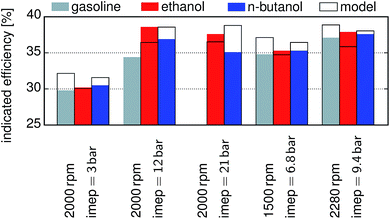 |
| | Fig. 5 Comparison of the model predictions with published data52 for different fuels and load points. Frames: the modelling results, filled shapes: published data: gray gasoline, red ethanol, blue n-butanol. | |
5.3 Loss analysis
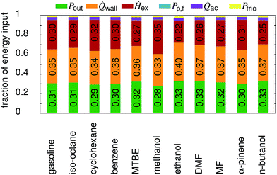
In Fig. 6 an overview on the energy distribution for each fuel is shown. It can be seen that the output power (Pout), the wall heat losses (![[Q with combining dot above]](https://www.rsc.org/images/entities/i_char_0051_0307.gif) wall) and the enthalpy of the exhaust gas (Ḣex) account for about 95% of the total energy input. In general, the wall heat losses as well as the power output increase with the compression ratio, while the enthalpy of the exhaust decreases. The peak pressure is a direct function of the compression ratio, and the pressure governs the wall heat losses. The decrease in exhaust enthalpy can be explained by the increased expansion in high compression ratio engines. Only methanol behaves differently. As many of the properties of methanol are extreme when compared to the other fuels, a detailed assessment is beyond the scope of this study. The major difference between n-butanol, ethanol and DMF is reflected in the friction losses which are 29% higher for ethanol and 8% lower for DMF than for n-butanol. The other shares vary less than 2% (again compared to n-butanol). Overall, this leads to a power output fraction of 33.3% for n-butanol, followed by ethanol (32.9%) and DMF (32.7%).
wall) and the enthalpy of the exhaust gas (Ḣex) account for about 95% of the total energy input. In general, the wall heat losses as well as the power output increase with the compression ratio, while the enthalpy of the exhaust decreases. The peak pressure is a direct function of the compression ratio, and the pressure governs the wall heat losses. The decrease in exhaust enthalpy can be explained by the increased expansion in high compression ratio engines. Only methanol behaves differently. As many of the properties of methanol are extreme when compared to the other fuels, a detailed assessment is beyond the scope of this study. The major difference between n-butanol, ethanol and DMF is reflected in the friction losses which are 29% higher for ethanol and 8% lower for DMF than for n-butanol. The other shares vary less than 2% (again compared to n-butanol). Overall, this leads to a power output fraction of 33.3% for n-butanol, followed by ethanol (32.9%) and DMF (32.7%).
 |
| | Fig. 6 Distribution of the total energy input at full load. Pp,f is the power supplied to the fuel pump, Pout the net power output of the engine, Pfric the friction losses within the engine, ![[Q with combining dot above]](https://www.rsc.org/images/entities/i_char_0051_0307.gif) wall the wall heat losses, wall the wall heat losses, ![[Q with combining dot above]](https://www.rsc.org/images/entities/i_char_0051_0307.gif) ac the heat transferred by the after-cooler, and Ḣex the enthalpy of the exhaust stream. ac the heat transferred by the after-cooler, and Ḣex the enthalpy of the exhaust stream. | |
5.4 Sensitivity analysis
The obtained Si for ηFL and PFL show a strong correlation that can be traced back to eqn (17). The SA results can therefore be plotted as Si for eCO2,FLversus Si for ηFL and PFL as depicted in Fig. 7. Herein, the dotted lines represent the threshold below which the factors can be assumed as non-influential.55 Three input factor groups (i–iii, marked by gray shaded areas) with comparable impact on the model outputs can be discerned. Highly influential factors in the group include (i) the fuel composition (x, y, z, v) and the vapor heat capacity cp,g. The importance of the former is related to the effect on the air-to-fuel ratio (AFR) and on the LHV, which defines the amount of fuel within the cylinder and the burnt gas composition. The least influential factors are grouped in (iii) and include parameters that only affect the fuel droplet evaporation rate. Within the varied parameter range, this rate is typically high enough to ensure complete evaporation before reaching the TDC. Both parameters might therefore be fixed without changing the variance of the three model outputs. The input factors of intermediate importance are grouped in (ii), including hvap, RON, ν, pvap and ρ.
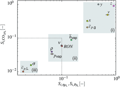 |
| | Fig. 7 Plot of sensitivity index Si for model output eCO2,FLversus Si for ηFL and PFL (circles represent the mean values while lines represent the respective span). Three gray-shaded areas (i–iii) mark input factor groups of similar importance. The dotted line indicates a threshold below which factors can be considered non-influential.55 | |
5.5 Single load points
In Table 4 the main results of the fuels are depicted. The compounds n-butanol, ethanol, and DMF show the highest efficiencies and power outputs. Their power output is very similar, while the efficiency of n-butanol at full load is slightly higher. The compression ratio for ethanol stands out as it is significantly higher than the values for all other fuels. It is in the range of a diesel engine rather than that of an SI engine. First tests to exploit this potential have already been conducted by converting a diesel engine to perform SI operation.56
Table 4 Overview on the performance of each fuel. ηFL efficiency at full load, ηPL efficiency at 2000 rpm and Pout = 6.6 kW, PFL power output at full load, eCO2 specific CO2 emissions
| Fuel |
η
FL [%] |
η
PL [%] |
P
FL [kW] |
e
CO2,FL [kg kWh−1] |
ε
CR [—] |
| Gasoline |
33.7 |
20.8 |
70.8 |
0.77 |
7.7 |
| Isooctane |
34.5 |
21.2 |
74.1 |
0.72 |
8.0 |
|
n-Heptane |
Knocking
|
| Cyclohexane |
32.3 |
20.1 |
69.4 |
0.80 |
7.3 |
| Benzene |
33.0 |
20.3 |
72.0 |
0.93 |
8.7 |
| MTBE |
35.7 |
21.6 |
75.6 |
0.72 |
9.4 |
| Methanol |
30.2 |
18.4 |
69.4 |
0.82 |
9.6 |
| Ethanol |
36.0 |
22.0 |
80.0 |
0.71 |
18.3 |
|
n-Butanol |
36.5 |
22.0 |
79.7 |
0.70 |
11.6 |
| MF |
34.6 |
21.0 |
76.7 |
0.92 |
10.4 |
| DMF |
35.9 |
21.7 |
79.2 |
0.85 |
10.0 |
| α-Pinene |
32.8 |
20.4 |
70.8 |
0.84 |
7.3 |
Although DMF has an RON of 119 and ethanol of 109, the optimum compression ratio is much lower for DMF than for ethanol. This suggests that other fuel properties also affect the optimum compression ratio. The maximum compression ratio is limited by the onset of knocking. According to the knock model the temperature at the TDC is one of the governing factors influencing the occurrence of knock. Besides the compression ratio, the enthalpy of vaporization, the vapor heat capacity as well as the air to fuel ratio influence the temperature (T2) at the TDC. In the case of DMF and ethanol, both cp,g and hvap have very different values.
In Fig. 8 the results of the full load point are summarized. n-Butanol and ethanol show the best overall performance followed by MTBE. DMF is an option if CO2 emissions are climate-neutral.
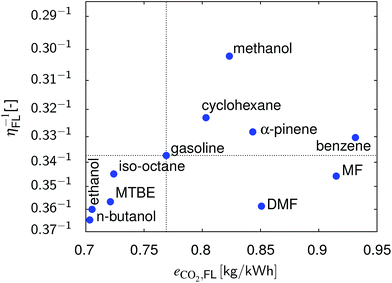 |
| | Fig. 8 Comparison of the different fuels with respect to η and CO2 emissions at full load and at their optimum compression ratio. | |
5.6 Cycle operation
The results (Table 5) are similar for all three cycles. α-Pinene and benzene are the only fuels yielding a lower consumption than gasoline. The efficiency is improved and the CO2 emissions are reduced for iso-octane, MTBE, ethanol and n-butanol. DMF and MF show higher efficiencies and higher CO2 emissions. With regard to CO2 emissions, ethanol and n-butanol are the most promising candidates with a reduction of roughly 8% compared to gasoline. MTBE and iso-octane cause a reduction of around 5%. All other fuels result in higher CO2 emissions over the driving cycles. The overall differences of the cycles can be attributed to the differences in the velocity profiles and thereby the required load.
Table 5 Results for the different cycles (CADC, WLTC, and NEDC)
|
|
CADC |
WLTC |
NEDC |
|
η
cyc [%] |
e
CO2,D [g km−1] |
Consumption [l/100 km] |
η
cyc [%] |
e
CO2,D [g km−1] |
Consumption [l/100 km] |
η
cyc [%] |
e
CO2,D [g km−1] |
Consumption [l/100 km] |
| Gasoline |
24.1 |
198 |
8.4 |
21.1 |
193 |
8.2 |
16.1 |
217 |
9.2 |
| Iso-octane |
24.6 |
187 |
8.8 |
21.5 |
182 |
8.6 |
16.5 |
204 |
9.6 |
| Cyclohexane |
23.2 |
206 |
8.5 |
20.3 |
201 |
8.3 |
15.6 |
225 |
9.3 |
| Benzene |
23.6 |
240 |
8.1 |
20.6 |
234 |
7.9 |
15.8 |
264 |
8.9 |
| MTBE |
25.3 |
188 |
10.2 |
22.1 |
183 |
9.9 |
16.9 |
205 |
11.2 |
| Methanol |
21.5 |
213 |
19.7 |
18.6 |
209 |
19.3 |
14.1 |
238 |
21.9 |
| Ethanol |
25.8 |
181 |
12.1 |
22.5 |
177 |
11.8 |
17.1 |
201 |
13.4 |
|
n-Butanol |
25.8 |
183 |
9.6 |
22.5 |
179 |
9.3 |
17.2 |
202 |
10.5 |
| DMF |
25.3 |
222 |
9.1 |
22.1 |
216 |
8.8 |
17.0 |
242 |
9.9 |
| MF |
24.5 |
238 |
9.7 |
21.4 |
232 |
9.5 |
16.3 |
261 |
10.7 |
| α-Pinene |
23.5 |
217 |
7.8 |
20.6 |
211 |
7.6 |
15.8 |
236 |
8.5 |
Another important fuel parameter, in particular from a consumer perspective, is the fuel consumption. Only benzene and α-pinene outperform gasoline. Methanol performs exceptionally poor with respect to fuel consumption. MTBE and, to a lower extent, MF also lead to a significant decrease in the achievable range. For n-butanol and ethanol, the fuel consumption is approximately 14% and 44% higher, respectively, compared to gasoline. DMF shows a consumption comparable to gasoline.
In Fig. 9 the results of the WLTC are summarized in terms of CO2 emissions per distance and consumption. There is no compound better than gasoline for both metrics. In terms of CO2 emissions, n-butanol and ethanol are very similar, with ethanol showing a significantly higher consumption, followed by MTBE and iso-octane. α-Pinene and benzene have the lowest fuel consumption instead.
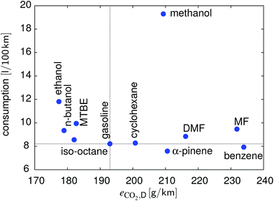 |
| | Fig. 9 Comparison of the different fuels with respect to consumption and CO2 emissions over the WLTC. | |
5.7 Further influences
The presented model covers first order effects only. Several other parameters have not been investigated, in particular the flame speed, soot formation and ignition timing.
In recent years soot formation became an issue for SI engines, too. The paths to soot formation are complex and depend largely on the combustion chemistry of the fuel. As the model is primarily intended as a screening tool for new fuels, these reaction pathways are unknown in most cases, making a priori modelling of soot emissions impossible. In any case a good preparation of the mixture may lead to lower soot emissions. If this is not sufficient particulate filters may provide a solution to the problem.
The flame speed influences the heat release rate and thus the pressure curve. The combustion within an engine is highly turbulent. Therefore, the turbulent flame speed is of interest which combines the laminar flame speed with the flow field in the cylinder. By assuming the same combustion for all fuels, the turbulence level within the cylinder is adapted to correct for deficiencies of the laminar flame speed. In practice, this is only possible within a limited range, as this may lead to excessive wall heat losses and extinction of the flame.
The ignition timing is considered implicitly: it is assumed that the engine control sets the ignition such that the combustion is achieved as assumed.
In summary it is important to note that the model focuses on first order effects and is in particular intended for fuels lacking experimental data to determine the potential of a certain fuel.
6 Conclusion
The development of a thermodynamic model of an SI DI ICE with particular focus on the influence of the fuel has allowed evaluation of the suitability of different compounds as a fuel for such an engine.
By means of GSA it could be shown that the influence of the liquid heat capacity and the surface tension of the fuel is negligible. The chemical composition and the vapor heat capacity are shown to be the major influential properties of a compound on the engine performance.
Among the alternative fuels considered in this study, the most promising candidate to replace gasoline is n-butanol, which shows a significant increase in efficiency as well as CO2 reduction potential. Ethanol behaves very similarly to n-butanol, with the exception of consumption which is considerably increased. They are followed by MTBE and iso-octane at the cost of somewhat higher CO2 emissions. DMF and MF increase the efficiency with a similar consumption to n-butanol, at the cost of significantly increased CO2 emissions. Methanol seems inferior to gasoline with respect to all parameters. α-Pinene performs somewhat worse than gasoline but shows the lowest consumption of all considered compounds including gasoline. This is in line with ref. 8 where the usage of α-pinene was proposed with a main focus on minimizing consumption. Cyclohexane shows the same consumption and higher CO2 emissions compared to gasoline.
All fuels show an optimum compression ratio between 7 and 12, with the exception of ethanol (18.3). High compression ratios do not pose any problems from a mechanical point of view. Talking about multi-fuel engines, the situation is different. Such an engine has to be operational with all possible kinds of fuels and therefore the compression ratio will need to be chosen such that all the fuels perform reasonably well. As a result, fuels with a high optimum compression ratio are not used to their full extent. In summary, n-butanol is the best alternative to gasoline, showing good full load performance, an acceptable increase in consumption and the second best performance at part load.
Conflicts of interest
There are no conflicts to declare.
Appendix
A Thermodynamic model
The modelling constants used in the following sections are listed in Table 6.
Table 6 Overview on the modelling constants and their value
| Name |
Symbol |
Value |
| Ambient temperature |
T
amb
|
298 K |
| Cylinder wall temperature |
![[T with combining macron]](https://www.rsc.org/images/entities/i_char_0054_0304.gif) w
w
|
470 K |
| Fuel injection nozzle diameter |
d
nozzle
|
300 μm |
| Peak pressure limitation |
p
peak
|
25 MPa |
| Fuel injection pressure |
p
fuel,inj
|
20 MPa |
| Minimum compression ratio |
ε
CR,min
|
5 |
| Maximum compression ratio |
ε
CR,max
|
20 |
| Minimum stepsize |
ΔεCR,min |
0.002 |
|
|
K
p
1
p
III
|
0.95 |
|
δ
valve,III
|
0.1 |
|
K
wh
|
12 (m2 s−1)0.2 |
|
K
q,tot
|
0.14 (m2 s−1)0.2 |
A.1 Intake.
Prior to intake, the air flows through the compressor of the turbocharger. The ideal after-cooler then cools the air stream down to ambient temperature (Tamb). Overall this leads to an increase in pressure by the compression ratio (Πc), while the temperature remains unchanged.
For describing the intake, compression (ΔTch) and wall heating (ΔTwh) effects are taken into account. It is assumed that no exhaust gas remains in the cylinder. The values for ΔTch and ΔTwh are defined by the following equations:19
| |  | (28) |
| |  | (29) |
| | | T1 = TIII + ΔTch + ΔTwh | (30) |
where
T1 denotes the in-cylinder temperature after intake,
S the stroke,
B the bore,
cm the mean piston velocity (defined as
cm = 2
SN),
![[T with combining macron]](https://www.rsc.org/images/entities/i_char_0054_0304.gif) w
w the mean cylinder wall temperature,
TIII the temperature prior to intake and
κ the heat capacity ratio. The empirical constants
Kp1pIII,
δvalve,III and
Kwh are chosen according to the recommendations by Boulouchos.
19
A.1.1 Fuel injection.
The initial droplet diameter (dd0)57 can be estimated based on the nozzle diameter (dnozzle), the Weber number (Wed) and the Reynolds number (Red).| | | dd0 = 3.67dnozzle(We0.5dRed)−0.259 | (31) |
| |  | (32) |
| |  | (33) |
The initial droplet velocity (uinj) is obtained from Bernoulli's equation, as
| |  | (34) |
The fuel injection pressure pfuel,inj is set to 20 MPa.
A.1.2 Droplet evaporation.
The Nusselt number (Nu) for a sphere within a flow field58 is given by eqn (35) as a function of the Prandtl number (Pr) and Reynolds number (Re).| | | Nu = 2 + 0.6Re1/2Pr1/3 | (35) |
Using the definition of the Nusselt number  , the heat flow to each droplet (
![[Q with combining dot above]](https://www.rsc.org/images/entities/i_char_0051_0307.gif) d) can be calculated as follows:
d) can be calculated as follows:
| |  | (36) |
with
kgas being the thermal conductivity of the surrounding gas mixture and
Tgas and
Td the temperatures of the gas mixture and of the droplet.
As proposed by Godsave,21 for fuel temperatures below the boiling point the d2-law is employed to describe the evolution of the droplet diameter (dd) with time.
| |  | (37) |
The evaporation parameter LA is calculated according to Ranz and Marshall.59
| |  | (38) |
where
| |  | (39) |
The mass transfer number Y1s is defined by Lefebvre60 as:
| |  | (40) |
The vapor pressure is calculated according to the Clausius–Clapeyron eqn (2). In the present case, the amount of evaporated fuel can be calculated from the difference in the diameter between the current and the preceding time step.
In case the fuel temperature reaches the boiling point, the amount of evaporated fuel is determined by the heat supplied divided by the heat of vaporization.
A.1.3 Compression.
The instantaneous wall heat transfer coefficient (αW) was initially described by Woschni61 and later improved by Hohenberg.22 According to Abedin et al.,62 the improved version gives significantly better results. Hohenberg's definition of the heat transfer coefficient is:| | | αW = 130V−0.06p0.8T−0.4(1.4 + cm)0.8 | (41) |
On the basis of this equation, the heat losses to the wall can be expressed as:
| | ![[Q with combining dot above]](https://www.rsc.org/images/entities/i_char_0051_0307.gif) w = αWAwall(φ(t))(T − w = αWAwall(φ(t))(T − ![[T with combining macron]](https://www.rsc.org/images/entities/i_char_0054_0304.gif) w) w) | (42) |
Using the first law of thermodynamics, the energy balance around the complete cylinder volume is described by:
| | nmix(Tgas(n+1)cV(n+1) − Tgas(n)cV(n)) = W − (nd![[Q with combining dot above]](https://www.rsc.org/images/entities/i_char_0051_0307.gif) d + d + ![[Q with combining dot above]](https://www.rsc.org/images/entities/i_char_0051_0307.gif) w)Δt w)Δt | (43) |
where
nmix denotes the total number of molecules within the cylinder,
nd the number of droplets, *
(n)/*
(n+1) the current/next iteration, respectively, and
W the work done due to compression. The work is defined by
| |  | (44) |
where
κ stands for the heat capacity ratio of the gas mixture.
A.2 Adaption of εCR.
The allowable maximum compression ratio is limited by knocking and thus depends on the RON of the fuel. The efficiency increases with the compression ratio until friction losses and wall heat losses become significant enough to reverse this effect. Therefore, an optimum for compression has to be determined for each fuel.
For the first run of the model, the compression ratio (εCR) is set to the minimum value (εCR,min) and engine simulation is performed. If either the knock index (kI < 1) or the peak pressure limitation (ppeak) is violated, the fuel is not suitable and the procedure is stopped.
As a next step, the maximum allowable compression ratio (εCR,max,ok) below the limit (εCR,max) is found by means of the bisection procedure.23 The minimum stepsize is chosen as ΔεCR,min. The maximum efficiency is searched for within the range of εCR ∈ [5, εCR,max,ok]. This is done by employing Brent's method63 to find the compression ratio for which the following condition is satisfied:  . Once this point has been identified, knocking and the peak pressure limitation are checked. If both parameters are fine, the engine parameters best suited for the fuel in question have been found. Otherwise, the bisection method23 is used to find the compression ratio giving a knock index of kI ≤ 0.999999.
B Heat transfer – compound dependence
The heat transfer coefficient (α) can be described by the following Nusselt number (Nu) correlation:depending on the Reynolds number (Re) and Prandtl number (Pr) as well as the constants C, β, and γ. Using the definition of these dimensionless quantities, the heat transfer coefficient can be described as| |  | (46) |
with k being the thermal conductivity of the gas, L the characteristic length, u the characteristic velocity and μ the dynamic viscosity of the gas. It is assumed that the characteristic velocity depends linearly on the mean piston speed, introducing two constants (C1,2)
The temperature dependence of the thermal conductivity as well as the dynamic viscosity are assumed to follow
| |  | (48) |
| |  | (49) |
The constants ε1,2 need to be determined based on measurements for each fluid. Applying all assumptions the heat transfer coefficient can be written as:
| |  | (50) |
| | ![[C with combining tilde]](https://www.rsc.org/images/entities/i_char_0043_0303.gif) = CC1γ = CC1γ | (51) |
following the argumentation of Hohenberg.
22L is expressed as

. Comparing
eqn (51) to the correlation proposed by Hohenberg
22 the following identities can be deduced by means of a coefficient comparison
| | | 0.4 = ε(air)1(β − γ) + ε(air)2(1 − β) | (54) |
| |  | (55) |
| |  | (56) |
| |  | (57) |
This finally leads to
| |  | (58) |
The relative deviation (Δα) with respect to the correlation by Hohenberg22 is
| |  | (59) |
| |  | (60) |
The relative deviation of the heat transfer coefficient of all fuels for which data were available, the fuel–air mixtures as well as their burnt gas mixtures are calculated based on data from DIPPR and mixing rules from Poling et al.64 The results are shown in Table 7. The measurement accuracy claimed by Hohenberg22 is around 20%. It is therefore concluded that the errors are within the measurement accuracy.
Table 7 List of heat transfer deviation, std: standard deviation
|
|
|
Mean (Δα) |
Mean (|Δα|) |
Std (Δα) |
| Fuel–air |
Heptane |
−7.12 |
10.09 |
8.9 |
| Iso-octane |
−7.05 |
10.03 |
8.87 |
| Benzene |
−3.71 |
7.17 |
7.31 |
| Cyclohexane |
−6.51 |
9.55 |
8.62 |
| Methanol |
−12.09 |
15.05 |
11.77 |
| Ethanol |
−9.5 |
12.45 |
10.31 |
| Butanol |
−8.06 |
11.05 |
9.5 |
| Burnt |
Heptane |
1.89 |
2.78 |
3.32 |
| Iso-octane |
2.42 |
2.93 |
3.29 |
| Benzene |
1.42 |
2.76 |
3.42 |
| Cyclohexane |
2.12 |
2.91 |
3.43 |
| Methanol |
−3.6 |
6.85 |
6.96 |
| Ethanol |
−0.48 |
3.52 |
4.19 |
| Butanol |
0.96 |
3.29 |
4.14 |
|
|
Overall |
−3.52 |
7.17 |
8.65 |
Table 8 Main properties of the engine and test bench used to acquire validation data
| Engine type |
Four stroke, gasoline, turbocharged |
| Fueling |
Direct injection |
| Emission legislation |
Euro 6 |
|
n
cyl
|
4 |
| Bore B |
87 mm |
| Stroke S |
90 mm |
| Compression ratio εCR |
10 |
| Fuel |
Market fuel fulfilling EN228, RON 98 |
| Engine test bench |
Horiba Dynas3 LI 250 |
| Automation and DAQ system |
Horiba STARS Engine |
| Fuel consumption measurement |
AVL 730 dynamic balance |
| Emission bench |
Horiba Mexa 9200 |
| Cylinder pressure sensing |
Kistler 6041 B sensor, water-cooled |
| Crank angle sensing |
Kistler 2614 encoder |
| Indication system |
Kistler KiBox |
C Friction mean effective pressure correlation
The properties of the fit for the fmep are listed below:
| Variable |
Mean |
Standard deviation |
p-Value |
| fmep0 [bar] |
0.3515315 |
0.0381548 |
6.40 × 10⁻¹⁶ |
|
β
0 [—] |
0.0054443 |
0.0002548 |
<2 × 10⁻¹⁶ |
|
β
1 [bar m−1 s−1] |
0.0455316 |
0.0076482 |
2.24 × 10⁻⁸ |
|
β
2 [bar (m−1 s−1)2] |
0.0012867 |
0.0003366 |
0.000203 |
Residual standard error: 0.08661 on 132 degrees of freedom.
Multiple R2: 0.9632.
Adjusted R2: 0.9624.
F-Statistic: 1151 on 3 and 132 DF.
p-Value: <2.2 × 10⁻¹⁶.
D Engine test bench configuration
Please see Table 8 for details of the main properties of the engine and test bench used to acquire validation data.
E Convergence
The employed EE method is a sampling-based approach to SA.45 While a too small quantity of a sample may not yield robust results, an excessively large one may not provide a significant improvement in precision. It is therefore important to investigate how robust the obtained SA results are to changes in sample size.
For this purpose, sub-samples of the original sample were taken and the sensitivity indices (see eqn (26)) and their uncertainty were calculated via the bootstrap technique.65 Based on the width of the 95% confidence intervals of the individual sensitivity indices, a summary statistic is calculated as
| |  | (61) |
where
Subi and
Slbi define the upper and lower bounds of the sensitivity index
Si and
M the number of input factors.
48
Fig. 10 presents the computed statistics for the three model outputs η, P and eCO2 as a function of the number of model evaluations. Herein, convergence is assumed to have been reached below a threshold of 0.05.48 The sensitivity indices for all three model outputs converge after 1.5 × 10⁵ to 2.7 × 10⁵ model evaluations.
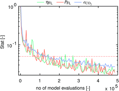 |
| | Fig. 10 Convergence statistics versus the number of model evaluations for η, P and eCO2. Convergence is assumed to have been reached below a threshold of 0.05.48 | |
Nomenclature
Variables
|
ε
tot
| Total energy input [J mol−1] |
|
η
| Efficiency [—] |
|
κ
| Heat capacity ratio [—] |
|
μ
| Friction coefficient [—] |
|
Π
| Pressure ratio [—] |
|
ρ
| Density [kg m−3] |
|
τ
ig
| Ignition delay [s] |
|
ε
CR
| Compression ratio [—] |
|
φ
| Crank angle [rad] |
|
A
| Area [m2] |
|
B
| Bore [m] |
|
c
| Specific molar heat capacity [J mol−1 K−1] |
![[c with combining macron]](https://www.rsc.org/images/entities/i_char_0063_0304.gif)
| Mass specific heat capacity [J kg−1 K−1] |
|
c
m
| Mean piston speed [m s−1] |
|
c
D
| Drag coefficient [—] |
|
e
| Emission [g] |
|
F
| Force [N] |
|
h
| Mol specific molar enthalpy [J mol−1] |
![[h with combining macron]](https://www.rsc.org/images/entities/i_char_0068_0304.gif)
| Mass specific enthalpy [J kg−1] |
|
M
| Molar mass [kg mol−1] |
|
m
| Mass [kg] |
|
N
| Rotational speed [rpm] |
|
P
| Power [W] |
|
p
| Pressure [Pa] |
|
Q
| Heat [J] |
|
S
| Stroke [m] |
|
s
| Entropy [J mol−1 K−1] |
|
T
| Temperature [K] |
|
t
| Time [s] |
|
V
| Volume [m3] |
|
v
| Number of nitrogen atoms [—] |
|
v
| Velocity [m s−1] |
|
W
| Work [J] |
|
x
| Number of carbon atoms [—] |
|
y
| Number of hydrogen atoms [—] |
|
z
| Number of oxygen atoms [—] |
Constants
|
g
| Gravitational acceleration = 9.81 m s−2 |
|
K
| Constant |
|
R
| Gas constant = 8.314 J mol−1 K−1 |
Subscripts
| acc | Acceleration |
| amb | Ambient |
| b | Burnt |
| bt | Turbine back pressure |
| c | Compressor |
| cyl | Cylinder |
|
D
| Displacement |
| ex | Exhaust |
| FL | Full load |
| g | Gaseous |
| in | Intake, input |
|
p
| Constant pressure |
| PL | Part load |
| ref | Reference |
| t | Turbine |
| tc | Turbocharger |
| tot | Total |
| ub | Unburnt |
|
V
| Constant volume |
| vap | Vapor |
| w | Wall |
Acknowledgements
Special thanks go to D. Wüthrich for his support in building the model and the countless hours of fruitful discussion. We would like to thank L. Bärtsch for the web and programming support and S. Müller for his help in getting the paper into its final form as well as K. Boulouchos (ETHZ) and C. Bach (Empa) for the time they spent to share their knowledge about engines and modelling with us. This work was supported by the SCCER BIOSWEET, via funding from the Commission for Technology and Innovation (Bern, Switzerland).
References
-
IEA, CO2 Emissions from Fuel Combustion 2013, IEA, 2013 Search PubMed.
- G. T. Kalghatgi, Int. J. Engine Res., 2014, 15, 383–398 CrossRef CAS.
- M. Contestabile, G. J. Offer, R. Slade, F. Jaeger and M. Thoennes, Energy Environ. Sci., 2011, 4, 3754 Search PubMed.
- S. Ramachandran and U. Stimming, Energy Environ. Sci., 2015, 8, 3313–3324 Search PubMed.
-
Strategic Research Agenda & Strategy Deployment Document, European Biofuels Technology Platform, CPL Press, 2008 Search PubMed.
- C. Wang, H. Xu, R. Daniel, A. Ghafourian, J. M. Herreros, S. Shuai and X. Ma, Fuel, 2013, 103, 200–211 CrossRef CAS.
- P. S. Nigam and A. Singh, Prog. Energy Combust. Sci., 2011, 37, 52–68 CrossRef CAS.
-
V. Raman, V. Sivasankaralingam, R. Dibble and S. M. Sarathy, SAE Technical Paper Series, 2016 Search PubMed.
- J. C. Serrano-Ruiz and J. A. Dumesic, Energy Environ. Sci., 2011, 4, 83–99 CAS.
- R. Luque, L. Herrero-Davila, J. M. Campelo, J. H. Clark, J. M. Hidalgo, D. Luna, J. M. Marinas and A. A. Romero, Energy Environ. Sci., 2008, 1, 542 CAS.
- C. Jin, M. Yao, H. Liu, C. f. F. Lee and J. Ji, Renewable Sustainable Energy Rev., 2011, 15, 4080–4106 CrossRef CAS.
-
T. Wallner, A. Ickes and K. Lawyer, Lecture Notes in Electrical Engineering, Springer Nature, 2012, pp. 15–26 Search PubMed.
- A. M. Pourkhesalian, A. H. Shamekhi and F. Salimi, Fuel, 2010, 89, 1056–1063 CrossRef CAS.
- J. Tirkey, H. Gupta and S. Shukla, Therm. Sci., 2009, 13, 113–130 CrossRef.
- A. Djouadi and F. Bentahar, Energy, 2016, 101, 211–217 CrossRef CAS.
- Y. Shen, J. Bedford and I. S. Wichman, Appl. Therm. Eng., 2009, 29, 2379–2385 CrossRef CAS.
-
S. Ramachandran, IMECS 2009: International Multi-Conference of Engineers and Computer Scientists, Vols I and II, 2009, pp. 2146–2151 Search PubMed.
- D. Mehrnoosh, H. A. Asghar and M. A. Asghar, J. Mech. Sci. Technol., 2012, 26, 2213–2225 CrossRef.
-
K. Boulouchos, Lecture Documents: IC-Engines and Propulsion Systems I, ETH Zürich, Switzerland, Autumn Semester, 2014 Search PubMed.
- S. Channiwala and P. Parikh, Fuel, 2002, 81, 1051–1063 CrossRef CAS.
-
G. Godsave, Symposium (International) on Combustion, 1953, vol. 4, pp. 818–830 Search PubMed.
-
G. F. Hohenberg, SAE Technical Paper Series, 1979 Search PubMed.
-
M. B. Allen and E. L. Isaacson, Numerical Analysis for Applied Science, John Wiley & Sons, Inc., 1997 Search PubMed.
- M. Thewes, M. Muther, A. Brassat, S. Pischinger and A. Sehr, SAE Int. J. Fuels Lubr., 2011, 5, 274–288 CrossRef.
-
A. M. Douaud and P. Eyzat, SAE Technical Paper Series, 1978 Search PubMed.
-
K. S. Chen and F. P. Flynn, SAE Technical Paper, 1965 Search PubMed.
-
H. Nguyen-Schäfer, Rotordynamics of Automotive Turbochargers, 2015, pp. 21–36 Search PubMed.
- Proposal for amendments to global technical regulation No. 15 on Worldwide harmonized Light vehicles Test Procedure (WLTP), 2016.
-
T. J. Barlow, S. Latham, I. S. McCrae and P. G. Boulter, A reference book of driving cycles for use in the measurement of road vehicle emissions, 2009 Search PubMed.
- UN Vehicle Regulations - 1958 Agreement - Uniform provisions concerning the approval of vehicles with regard to the emission of pollutants according to engine fuel requirements, 2015.
-
T. Schütz, Hucho - Aerodynamik des Automobils, Springer Vieweg, 6th edn, 2013 Search PubMed.
- Design Institute for Physical Properties, DIPPR Project 801-Full Version, Design Institute for Physical Property Research/AIChE, 2005; 2008; 2009; 2010; 2011; 2012; 2015.
-
J. B. Heywood, Internal Combustion Engine Fundamentals, McGraw-Hill Education Ltd, 1989 Search PubMed.
- L. M. Rodríguez-Antón, F. Gutiérrez-Martín and C. Martinez-Arevalo, Fuel, 2015, 156, 81–86 CrossRef.
-
R. Pischinger, M. Klell and T. Sams, Thermodynamik der Verbrennungskraftmaschine, Springer-Verlag KG, 2009 Search PubMed.
-
J. Yanowitz, E. Christensen and R. L. McCormick, Utilization of Renewable Oxygenates as Gasoline Blending Components, 2011, DOI:10.2172/1024518.
-
A. P. Institute, Technical Data Book - Petroleum Refining, 6th edn, 1997 Search PubMed.
- W.-Q. Han and C.-D. Yao, Fuel, 2015, 150, 29–40 CrossRef CAS.
-
H. Hamid, Handbook of MTBE and Other Gasoline Oxygenates (Chemical Industries), CRC Press, 2004 Search PubMed.
- J. E. Anderson, U. Kramer, S. A. Mueller and T. J. Wallington, Energy Fuels, 2010, 24, 6576–6585 CrossRef CAS.
-
P. J. Linstrom and W. G. Mallard, NIST Chemistry WebBook, NIST Standard Reference Database Number 69, National Institute of Standards and Technology, Gaithersburg MD, 20899, 2005 Search PubMed.
- M. Thewes, M. Muether, S. Pischinger, M. Budde, A. Brunn, A. Sehr, P. Adomeit and J. Klankermayer, Energy Fuels, 2011, 25, 5549–5561 CrossRef CAS.
- S. Zhong, R. Daniel, H. Xu, J. Zhang, D. Turner, M. L. Wyszynski and P. Richards, Energy Fuels, 2010, 24, 2891–2899 CrossRef CAS.
- G. Chen, Y. Shen, Q. Zhang, M. Yao, Z. Zheng and H. Liu, Energy, 2013, 54, 333–342 CrossRef CAS.
- A. Saltelli, M. Ratto, S. Tarantola and F. Campolongo, Chem. Rev., 2012, 112, PR1–PR21 CrossRef PubMed.
- M. D. McKay, R. J. Beckman and W. J. Conover, Technometrics, 1979, 21, 239–245 Search PubMed.
- F. Campolongo, A. Saltelli and J. Cariboni, Comput. Phys. Commun., 2011, 182, 978–988 CrossRef CAS.
- F. Sarrazin, F. Pianosi and T. Wagener, Environ. Model. Software, 2016, 79, 135–152 CrossRef.
-
S. J. Pachernegg, SAE Technical Paper Series, 1969 Search PubMed.
-
A. B. Greene and G. G. Lucas, The testing of internal combustion engines, The English Universities Press, Ltd, 1969 Search PubMed.
- G. Rizzoni, L. Guzzella and B. Baumann, IEEE ASME Trans. Mechatron., 1999, 4, 246–257 CrossRef.
- A. Brassat, M. Thewes, M. Müther and S. Pischinger, Motortech. Z., 2011, 72, 988–995 CrossRef.
- T. Venugopal and A. Ramesh, Int. J. Energy Res., 2013, 38, 1060–1074 CrossRef.
- S. Szwaja and J. Naber, Fuel, 2010, 89, 1573–1582 CrossRef CAS.
- P. A. Vanrolleghem, G. Mannina, A. Cosenza and M. B. Neumann, J. Hydrol., 2015, 522, 339–352 CrossRef.
-
M. Brusstar, M. Stuhldreher, D. Swain and W. Pidgeon, SAE Technical Paper Series, 2002 Search PubMed.
- K. H. Kwak, D. Jung and C. Borgnakke, Int. J. Engine Res., 2013, 15, 488–503 CrossRef.
-
F. P. Incropera, D. P. Dewitt, T. L. Bergman and A. S. Lavine, Principles of heat and mass transfer, John Wiley & Sons (Asia), Singapore, 7th edn, 2013 Search PubMed.
- W. Ranz and W. Marshall, Chem. Eng. Prog., 1952, 48, 141–146 CAS.
-
A. H. Lefebvre, Atomization and sprays, CRC Press/Taylor & Francis, Boca Raton, 1989 Search PubMed.
- G. Woschni, SAE Trans., 1968, 76, 176 Search PubMed.
- M. Abedin, H. Masjuki, M. Kalam, A. Sanjid, S. A. Rahman and B. Masum, Renewable Sustainable Energy Rev., 2013, 26, 20–33 CrossRef.
- R. P. Brent, Comput. J., 1971, 14, 422–425 CrossRef.
-
B. E. Poling, J. M. Prausnitz and J. P. O'Connell, The properties of gases and liquids, McGraw-Hill, 5th edn, 2001 Search PubMed.
-
B. Efron and R. Tibshirani, An introduction to the bootstrap, Chapman & Hall, New York, 1993, p. 436 Search PubMed.
Footnote |
| † Supporting data can be found at: http://fuel-simulation.psi.ch. |
|
| This journal is © The Royal Society of Chemistry 2017 |
 a,
Patrik
Soltic
 b,
Philip
Edinger
c,
Alexander
Wokaun
a and
Frédéric
Vogel
 *ad
*ad
![[Q with combining dot above]](https://www.rsc.org/images/entities/i_char_0051_0307.gif) wall within the cylinder are accounted for. The model is limited to fuels that are liquid under ambient conditions.
wall within the cylinder are accounted for. The model is limited to fuels that are liquid under ambient conditions.
![[c with combining macron]](https://www.rsc.org/images/entities/i_char_0063_0304.gif) p,g
p,g
![[c with combining macron]](https://www.rsc.org/images/entities/i_char_0063_0304.gif) p,L
p,L
![[h with combining macron]](https://www.rsc.org/images/entities/i_char_0068_0304.gif) vap
vap


 . The ignition delay (τig) is approximated by using the correlation proposed by Douaud and Eyzat.25


![[thin space (1/6-em)]](https://www.rsc.org/images/entities/char_2009.gif) 33
33![[thin space (1/6-em)]](https://www.rsc.org/images/entities/char_2009.gif) 34
34![[thin space (1/6-em)]](https://www.rsc.org/images/entities/char_2009.gif) 35
35![[thin space (1/6-em)]](https://www.rsc.org/images/entities/char_2009.gif) 36
36![[thin space (1/6-em)]](https://www.rsc.org/images/entities/char_2009.gif) 33
33![[thin space (1/6-em)]](https://www.rsc.org/images/entities/char_2009.gif) 36
36![[thin space (1/6-em)]](https://www.rsc.org/images/entities/char_2009.gif) 37
37![[thin space (1/6-em)]](https://www.rsc.org/images/entities/char_2009.gif) 38
38![[thin space (1/6-em)]](https://www.rsc.org/images/entities/char_2009.gif) 39
39![[thin space (1/6-em)]](https://www.rsc.org/images/entities/char_2009.gif) 40
40![[thin space (1/6-em)]](https://www.rsc.org/images/entities/char_2009.gif) 36
36![[thin space (1/6-em)]](https://www.rsc.org/images/entities/char_2009.gif) 36
36![[thin space (1/6-em)]](https://www.rsc.org/images/entities/char_2009.gif) 36
36![[thin space (1/6-em)]](https://www.rsc.org/images/entities/char_2009.gif) 41
41![[thin space (1/6-em)]](https://www.rsc.org/images/entities/char_2009.gif) 41
41![[thin space (1/6-em)]](https://www.rsc.org/images/entities/char_2009.gif) 41
41![[thin space (1/6-em)]](https://www.rsc.org/images/entities/char_2009.gif) 42
42![[thin space (1/6-em)]](https://www.rsc.org/images/entities/char_2009.gif) 36
36![[thin space (1/6-em)]](https://www.rsc.org/images/entities/char_2009.gif) 43
43![[thin space (1/6-em)]](https://www.rsc.org/images/entities/char_2009.gif) 41
41![[thin space (1/6-em)]](https://www.rsc.org/images/entities/char_2009.gif) 41
41![[thin space (1/6-em)]](https://www.rsc.org/images/entities/char_2009.gif) 41
41![[thin space (1/6-em)]](https://www.rsc.org/images/entities/char_2009.gif) 44
44![[thin space (1/6-em)]](https://www.rsc.org/images/entities/char_2009.gif) 36
36![[thin space (1/6-em)]](https://www.rsc.org/images/entities/char_2009.gif) 8
8![[thin space (1/6-em)]](https://www.rsc.org/images/entities/char_2009.gif) 8
8![[thin space (1/6-em)]](https://www.rsc.org/images/entities/char_2009.gif) 8
8![[thin space (1/6-em)]](https://www.rsc.org/images/entities/char_2009.gif) 8
8
 , averaged over n calculated EEs and its normalized form Si are measures of the total sensitivity of the ith of M input factors.48

![[Q with combining dot above]](https://www.rsc.org/images/entities/i_char_0051_0307.gif) wall) and the enthalpy of the exhaust gas (Ḣex) account for about 95% of the total energy input. In general, the wall heat losses as well as the power output increase with the compression ratio, while the enthalpy of the exhaust decreases. The peak pressure is a direct function of the compression ratio, and the pressure governs the wall heat losses. The decrease in exhaust enthalpy can be explained by the increased expansion in high compression ratio engines. Only methanol behaves differently. As many of the properties of methanol are extreme when compared to the other fuels, a detailed assessment is beyond the scope of this study. The major difference between n-butanol, ethanol and DMF is reflected in the friction losses which are 29% higher for ethanol and 8% lower for DMF than for n-butanol. The other shares vary less than 2% (again compared to n-butanol). Overall, this leads to a power output fraction of 33.3% for n-butanol, followed by ethanol (32.9%) and DMF (32.7%).
wall) and the enthalpy of the exhaust gas (Ḣex) account for about 95% of the total energy input. In general, the wall heat losses as well as the power output increase with the compression ratio, while the enthalpy of the exhaust decreases. The peak pressure is a direct function of the compression ratio, and the pressure governs the wall heat losses. The decrease in exhaust enthalpy can be explained by the increased expansion in high compression ratio engines. Only methanol behaves differently. As many of the properties of methanol are extreme when compared to the other fuels, a detailed assessment is beyond the scope of this study. The major difference between n-butanol, ethanol and DMF is reflected in the friction losses which are 29% higher for ethanol and 8% lower for DMF than for n-butanol. The other shares vary less than 2% (again compared to n-butanol). Overall, this leads to a power output fraction of 33.3% for n-butanol, followed by ethanol (32.9%) and DMF (32.7%).


![[T with combining macron]](https://www.rsc.org/images/entities/i_char_0054_0304.gif) w
w


![[T with combining macron]](https://www.rsc.org/images/entities/i_char_0054_0304.gif) w the mean cylinder wall temperature, TIII the temperature prior to intake and κ the heat capacity ratio. The empirical constants Kp1pIII, δvalve,III and Kwh are chosen according to the recommendations by Boulouchos.19
w the mean cylinder wall temperature, TIII the temperature prior to intake and κ the heat capacity ratio. The empirical constants Kp1pIII, δvalve,III and Kwh are chosen according to the recommendations by Boulouchos.19


 , the heat flow to each droplet (
![[Q with combining dot above]](https://www.rsc.org/images/entities/i_char_0051_0307.gif) d) can be calculated as follows:
d) can be calculated as follows:


![[Q with combining dot above]](https://www.rsc.org/images/entities/i_char_0051_0307.gif) w = αWAwall(φ(t))(T −
w = αWAwall(φ(t))(T − ![[T with combining macron]](https://www.rsc.org/images/entities/i_char_0054_0304.gif) w)
w)![[Q with combining dot above]](https://www.rsc.org/images/entities/i_char_0051_0307.gif) d +
d + ![[Q with combining dot above]](https://www.rsc.org/images/entities/i_char_0051_0307.gif) w)Δt
w)Δt
 . Once this point has been identified, knocking and the peak pressure limitation are checked. If both parameters are fine, the engine parameters best suited for the fuel in question have been found. Otherwise, the bisection method23 is used to find the compression ratio giving a knock index of kI ≤ 0.999999.


![[C with combining tilde]](https://www.rsc.org/images/entities/i_char_0043_0303.gif) = CC1γ
= CC1γ . Comparing eqn (51) to the correlation proposed by Hohenberg22 the following identities can be deduced by means of a coefficient comparison


![[c with combining macron]](https://www.rsc.org/images/entities/i_char_0063_0304.gif)
![[h with combining macron]](https://www.rsc.org/images/entities/i_char_0068_0304.gif)

