Multi-scale modeling of an amine sorbent fluidized bed adsorber with dynamic discrepancy reduced modeling
Received
22nd March 2017
, Accepted 9th June 2017
First published on 9th June 2017
Abstract
Inaccuracy in chemical kinetic models is a problem that affects the reliability of large-scale process models. Detailed and accurate kinetic models could improve this situation, but such models are often too computationally intensive to utilize at process scales. This work presents a method for bridging the kinetic and process scales while incorporating experimental data in a Bayesian framework. “Dynamic Discrepancy Reduced Modeling” (DDRM) enables the use of complex chemical kinetic models at the process scale. DDRM inserts Gaussian process (GP) stochastic functions into the first-principles dynamic model form, enabling a sharp reduction in model order. Uncertainty introduced through the order reduction is quantified through Bayesian calibration to bench-scale experimental data. The use of stochastic functions within the dynamic chemical kinetic model enables this uncertainty to be correctly propagated to the process scale. The model reduction and uncertainty quantification framework was applied to a reaction–diffusion model of mesoporous silica-supported, amine impregnated sorbents; model order reduction of over an order of magnitude was achieved through a sharp reduction in the resolution of the approximate solution for diffusion. GPs of the Bayesian smoothing splines analysis of variance (BSS-ANOVA) variety were applied to the diffusion coefficients and equilibrium constants in the model. The reduced model was calibrated using experimental dynamic thermogravimetric data, with prior probability distributions for physical model parameters derived from quantum chemical calculations. Model and parameter uncertainties represented in the posterior distribution were propagated to a bubbling fluidized-bed adsorber simulation implemented in Aspen Custom Modeler. This work is the first significant demonstration of the dynamic discrepancy technique to produce robust reduced order models for bench-to-process multi-scale modeling and serves as a proof-of-concept.
1 Introduction
CO2, which is responsible for about 64% of the total enhanced greenhouse effect, is the most important contributor to global warming both in terms of current impact and the rate of increase.1 The concentration of CO2 in the atmosphere has increased from 280 ppm to 400 ppm in the last 50 years and may reach 570 ppm by the year 2100, causing around a 1.9 °C rise of the global mean temperature.2,3 Decreasing CO2 emissions is thus urgent, and large-scale sources such as fossil fueled power plants are among the most important targets for emissions curbs.
Carbon capture and storage (CCS) technology is undergoing serious consideration as a method to reduce the emission of CO2 from power plants.4–9 However, the traditional timeline to advance new technologies from laboratory to industrial-scale deployment in the power industry takes twenty to thirty years.10 Part of the reason for this is that the results of bench and laboratory-scale experiments are difficult to utilize for predicting performance of large-scale processes.
Advances in multi-scale modeling have great potential to significantly decrease the time needed for deployment of carbon capture technologies.11,12 The U.S. Department of Energy's Carbon Capture Simulation Initiative (CCSI) focuses on the development of multi-scale models and computational tools for accelerating the development and scale-up of new carbon capture technologies for large-scale power plants; the project involves five national laboratories, five universities and more than twenty industrial partners.13,14 The quantification of uncertainty in chemical kinetic models and its propagation to larger-scale simulations has been an important part of the project.10
Mesoporous silica-supported, amine-impregnated (SSA) solid sorbents were one of the CO2 capture materials chosen to demonstrate the capabilities of the CCSI Toolset. These sorbents present a complex set of behaviors, especially with respect to the influence of H2O on the diffusion rate and effective capacity of the sorbent for CO2.15,16 A physical model, consistent with the known experimental behavior and quantum chemical calculations, has been developed.15–17 This thermodynamic and kinetic reaction–diffusion model, which considers a number of diffusive intermediates, is considerably more complex than chemical kinetic models typically employed in device models for large-scale process simulations. The challenge is to reduce the computational burden of the kinetic model to the point that it can be used in a process-scale simulation, while retaining the basic physics of the model and providing a vehicle for uncertainty quantification.
This challenge was met using dynamic discrepancy reduced modeling (DDRM), a new technique which is introduced in this article. DDRM is a methodology that reduces the order of dynamic systems by eliminating intermediate states (those that are not end points in the dynamic network) from the system. The model variability that is lost through the order reduction is replaced by incorporating Gaussian process (GP) stochastic functions into the model. The reduction is accomplished in such a manner that important features of the original dynamic system are retained. The GPs are discrepancy functions in that they contain the error of the reduced order model with respect to the original, and also potentially the error of the original model form with respect to reality. DDRM as such is a mixture of first-principles and empirical order reduction; DDRM models incorporate experimental results (or, one could imagine, the results of high-fidelity models) through the use of discrepancy functions, while retaining the important features of first-principles model forms.
DDRM is a technique that is based on the “dynamic discrepancy” method for model-based Bayesian calibration in dynamic systems.18 The key to the dynamic discrepancy technique is the intrusive use of stochastic discrepancy functions within the dynamic system itself. Used intrusively, discrepancy functions depend, in a simple fashion, on the states of the system. By contrast, model discrepancy functions applied outside of the dynamic model must depend on the Hilbert space of time-dependent functions of the system's inputs (such as temperature and concentrations of reactants and products) in order to properly account for extrapolations through that space; this is, generally speaking, completely impractical. Because propagation of uncertainty in a chemical kinetic model calibrated to bench-scale experiments to the process-scale almost inescapably involves such extrapolation, the dynamic discrepancy approach is essential for rigorous bench-to-process scale-bridging.
The stochastic dynamic systems resulting from the dynamic discrepancy technique are integrated during the process of model calibration to experimental datasets using Markov chain Monte Carlo (MCMC) sampling routines. Crucial to this capability is the nature of the GPs used for the discrepancy functions, which are of the Bayesian smoothing spline analysis of variance (BSS-ANOVA) variety.19 BSS-ANOVA GPs can be decomposed in such a manner that the stochasticity in the function resides wholly in a set of correlated parameters, the posterior distribution of which are estimated through the MCMC process.
The methodology of Bayesian calibration of computer models to data using discrepancy functions was pioneered by Kennedy and O'Hagan.20 This framework has been used for calibration and uncertainty quantification in many different areas, such as forest models,21,22 thermal problems,23,24 biogeochemical models,25 water quality,26,27 hydrological models,28,29 computational fluid dynamics models,30,31 and carbon capture.18,32–35 Work at Georgia Institute of Technology has used Bayesian calibration to quantify both epistemic and aleatory uncertainty in amine-based CO2 sorbents.36,37
2 Chemistry model
Derived using quantum chemical calculations and experimental results, a reaction–diffusion model has been proposed to describe the CO2 adsorption process in amine sorbents.16 In this model, the mechanism of CO2 diffusion in polymeric amines such as polyethylenimine (PEI) is zwitterion hopping. Under humid conditions, comparatively rare zwitterions can be stabilized by nearby amine and water molecules. Zwitterions form at the gas–amine interface and diffuse into the amine bulk to form carbamates. The chemical model is| |  | (1) |
| |  | (2) |
| |  | (3) |
| |  | (4) |
| |  | (5) |
The diffusive intermediates – amine-stabilized zwitterions, adsorbed water, and water-stabilized zwitterions – are denoted z1, z2, and z3, respectively. Carbamates – ammonium carbamate and hydronium carbamate – are denoted x and y, respectively. Assuming physisorption reactions at the surface are in equilibrium, the site fractions of diffusive intermediates at the surface are
where
PCO2 and
PH2O are the partial pressures of CO
2 and H
2O in the gas, and
κ1,
κ3, and
κ4 are the equilibrium constants of reactions (1), (3) and (4), respectively.
S is the free amine site fraction. The subscript “s” denotes the value at the gas–amine interface.
The rate equations for the formation of ammonium carbamates and hydronium carbamates are
| |  | (9) |
| |  | (10) |
where (
k2,
k5) and (
k−2,
k−5) are the forward and backward reaction rate constants of (2) and (5), respectively; with
κ2 =
k2/
k−2 and
κ5 =
k−2/
k−5. Equilibrium and rate constants are related to reaction enthalpy, entropy and activation enthalpy in the usual manner:
| |  | (11) |
| |  | (12) |
where
γi is a preexponential factor. Similarly, the transport coefficients (formulated as mobilities) of three diffusive intermediates are related to activation enthalpy for hopping:
| |  | (13) |
where
ζbi is a parameter that depends on the average geometry surrounding the diffusing species and the frequency of collisions with other amine sites.
The total number of model parameters including microstructural parameters, material properties, thermodynamic parameters, kinetic parameters and transport parameters is 23: θ = [θ1,…,θ23]T. A summary of input, output and model parameters appears in Table 1.
Table 1 Summary of inputs, outputs and reaction–diffusion model parameters
| Functional input profile (potential system conditions) ζ(t) |
|
ξ
1: temperature T |
|
ξ
2: partial pressure of CO2 |
|
ξ
3: partial pressure of H2O |
| Experimental outputs and state variables x and y |
|
x: weight fraction of ammonium carbamate |
|
y: weight fraction of hydronium carbamate |
| Model parameters |
|
θ
1: r3, diameter |
|
θ
2: f, estimated parameter |
|
θ
3: amine site density |
|
θ
4: nv, enthalpy of reaction 1 |
|
θ
5: ΔH1, entropy of reaction 1 |
|
θ
6: ΔS1, enthalpy of reaction 2 |
|
θ
7: ΔH2, entropy of reaction 2 |
|
θ
8: ΔH‡2, activation energy of reaction 2 |
|
θ
9: log10(γ2), preexponential parameter of reaction 2 |
|
θ
10: ΔH3, enthalpy of reaction 3 |
|
θ
11: ΔS3, entropy of reaction 3 |
|
θ
12: ΔH4, enthalpy of reaction 4 |
|
θ
13: ΔS4, entropy of reaction 4 |
|
θ
14: ΔH5, enthalpy of reaction 5 |
|
θ
15: ΔS5, entropy of reaction 5 |
|
θ
16: ΔH‡5, activation energy of reaction 5 |
|
θ
17: log10(γ5), preexponential parameter of reaction 5 |
θ
18:  , activation energy of z1 , activation energy of z1 |
|
θ
19: log10(ζb1), preexponential parameter of z1 |
θ
20:  , activation energy of z2 , activation energy of z2 |
|
θ
21: log10(ζb2), preexponential parameter of z2 |
θ
22:  , activation energy of z3 , activation energy of z3 |
|
θ
23: log10(ζb3), preexponential parameter of z3 |
3 Statistical methods
3.1 Bayesian calibration
Bayesian inference treats deterministic quantities such as physical model parameters as random variables, reflecting lack of knowledge (epistemic uncertainty). A Bayesian analysis begins with a prior distribution that represents current understanding about the quantities of interest from previous experience. The prior is combined with relevant data (observations) to yield the posterior distribution, which represents the new state of knowledge about the quantity after the data has been considered. The mathematical relationship between the prior, the observations, and the posterior is Bayes' theorem:| |  | (14) |
where ![[scr P, script letter P]](https://www.rsc.org/images/entities/char_e52f.gif) (θ∣Z) is the posterior: the probability of θ given dataset Z;
(θ∣Z) is the posterior: the probability of θ given dataset Z; ![[scr P, script letter P]](https://www.rsc.org/images/entities/char_e52f.gif) (Z∣θ) is the likelihood: the probability of observing the data given θ, which must include a model for the observation error; and
(Z∣θ) is the likelihood: the probability of observing the data given θ, which must include a model for the observation error; and ![[scr P, script letter P]](https://www.rsc.org/images/entities/char_e52f.gif) (θ) is the prior. The integral in the denominator is the probability of observing the particular dataset Z (Z is considered to be an observation of a stochastic variable
(θ) is the prior. The integral in the denominator is the probability of observing the particular dataset Z (Z is considered to be an observation of a stochastic variable  ) over all possible values of θ, called marginal likelihood or marginal density of the observations.
Kennedy and O'Hagan introduced a method for model calibration that includes a quantification of error in the model itself.20 In the Kennedy–O'Hagan approach, the statistical model for the data is
| |  | (15) |
where
M is the model,
δ is the model discrepancy and
ε is the observation error.
3.2 Dynamic discrepancy
Dynamic discrepancy18 is a variation of the Kennedy–O′Hagan approach that applies to systems in which the model M is dynamic, meaning that it will be difficult to build an additive discrepancy term in (15) that will accurately represent the error. Dynamic discrepancy replaces (15) with a new model:| |  | (16) |
The stochastic dynamic system can be solved and the joint posterior for (θ,δ) can be obtained using MCMC sampling if a judicious choice is made for the form of the discrepancy GP.
The BSS-ANOVA GP framework was introduced by Reich et al.19 The discrepancy function δ can be formulated using the BSS-ANOVA GP model19 and provides two critical advantages for the model (16). Most importantly, it relegates stochasticity in the GP to a set of coefficients β, which enables the deterministic evaluation of a likelihood function based on (16) when β is fixed. It also improves the computational efficiency by scaling linearly with the number of data points, as opposed to ![[scr O, script letter O]](https://www.rsc.org/images/entities/char_e52e.gif) (N3) for a traditional GP.18,38
(N3) for a traditional GP.18,38
The discrepancy function can be subjected to an ANOVA decomposition:
| |  | (18) |
where
β0 ∼
N(0,
ς02), and each main effect functional component
δr ∼
GP(0,
ςr2K1).
K1 is the BSS-ANOVA covariance generating kernel:
19| |  | (19) |
where
Bi is the
ith Bernoulli polynomial. Two-way interaction functions
δr,r′ ∼
GP(0,
ςr,r′2K2), where
| | | K2((u,v),(u′,v′)) = K1(u,u′)K1(v,v′) | (20) |
are dyadic products of the first-order kernels. Three-way or higher order interaction functional components are defined in an analogous fashion.
Each functional component in (18) can be further written as an orthogonal basis expansion following a Karhunen–Loéve decomposition:19
| |  | (21) |
where
τr,l =
λlςr2, with
λl the eigenvalue corresponding to the eigenfunction
ϕl produced in the Karhunen–Loéve (KL) expansion.
39,40 The eigenfunctions are orthogonal, spectral, nonparametric and ordered. The first nine functions are shown in
Fig. 1.
38 It was suggested by Storlie,
et al. that 25 terms retained in the expansion prior to truncation is often more than sufficient for most problems.
41 In many problems, it is sufficient to include only main effects and two-way interactions in the expansion. Considering only two-way interactions,
(18) becomes
| |  | (22) |
| |  | (23) |
where
j indexes over the
J functional components included in the discrepancy realization, and
l indexes over the number of basic functions
Lδj used for the
jth functional component of the discrepancy representation.
βj,l,
ϕj,l, and
τj would correspond to a particular term in the expansion of
(21) for the
jth functional component.
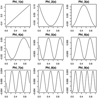 |
| | Fig. 1 First nine eigenfunctions from the Karhunen–Loéve expansion for a main effect function from the BSS-ANOVA covariance. | |
3.3 Reduced order model
3.3.1 Interactions.
The model as presented in sec. 2 above assumes ideal thermodynamics and kinetics; that is, it does not consider any interactions (aside from entropic interactions related to site occupancy) among the various chemical species appearing in the model.16 However, it is clear from the thermogravimetric analysis (TGA) experiments reported in this work that some non-idealities must be considered. One way to introduce such interactions in a continuum-level model is to explicitly consider associates among species; however, this tends to increase the complexity of the model. Discrepancy functions incorporated into the model can also treat interactions in an effective sense; for instance, the influence of interactions on the thermodynamics can be captured by applying discrepancy functions to the equilibrium constants:| |  | (24) |
such that the new, interaction-sensitive quantity κE depends now on the relevant thermodynamic quantities of partial pressure p and the temperature T. For the current study, for each of the reactions appearing in the model:‡| |  | (25) |
| |  | (26) |
| |  | (27) |
| |  | (28) |
| |  | (29) |
3.4 Implementation
3.4.1 Monte Carlo sampling.
Because of the intractability of the integral in the denominator on the right-hand side of eqn (14), a numerical simulation is required to obtain samples from the posterior distribution. MCMC sampling42,43 was used to obtain the posterior distributions of θ, δ and σ2. In each iteration of the routine, a set of model parameters θ and model discrepancy parameters β was proposed, the likelihood was evaluated, and the proposal was either accepted or rejected using the Metropolis–Hastings (MH) criterion.42 Taking advantage of an inverse gamma prior that is conjugate to the white noise model for the likelihood, Gibbs updates44 were used to obtain samples for the observation error variance σ2.
Block proposals for the parameters subject to MH sampling greatly decreased the time required for a single Monte Carlo step, which occurs when a new proposal for each parameter has been evaluated. Block proposals for the physical parameters were made using an adaptive, multivariate normal proposal distribution.45 A random vector was drawn from the multivariate normal distribution with a mean vector ![[small theta, Greek, macron]](https://www.rsc.org/images/entities/i_char_e0c9.gif) = [
= [![[small theta, Greek, macron]](https://www.rsc.org/images/entities/i_char_e0c9.gif) 1,...,
1,...,![[small theta, Greek, macron]](https://www.rsc.org/images/entities/i_char_e0c9.gif) 23] fixed at the current point in the random walk, and covariance matrix V is the empirical covariance of a subset of the previously accepted values in the MCMC chain:
23] fixed at the current point in the random walk, and covariance matrix V is the empirical covariance of a subset of the previously accepted values in the MCMC chain:
| |  | (34) |
The covariance matrix was initialized and recalculated every 1000 MCMC steps based on the last 2000 samples. It then was used as the covariance matrix for the next 1000 proposals. An adjustable multiplier on the covariance guides a reasonable acceptance rate of the proposal. After burn-in, the covariance matrix is fixed at the final proposal covariance.
For δ, all the β coefficients for each main effect and second order interaction coefficients (e.g.eqn (21)) were updated simultaneously using an adaptive multivariate normal proposal as described above. After a sufficient number of MCMC iterations, the samples of θ and β (and other parameters) will converge to its stationary distribution; this is the posterior distribution of the model parameters, model discrepancy parameters, and observation error parameters.
3.4.2 Prior distribution.
To complete the model specification, prior distributions are required for θ, δ, and σ2. Priors for some of the model parameters θ are derived from ab initio quantum chemistry calculations or from scientific literature and are specified using a normal distribution. The details of the quantum chemistry methods used to obtain these prior can be found in ref. 16. The model for δ in (22) requires a prior specification for τj's from (23). A diffuse inverse gamma prior is chosen for the τj's to promote better mixing of β and an inverse gamma prior is chosen as well for σ2. The selected priors for the τj's and σ2 are conjugate to the normal distribution of β's and the likelihood respectively, which ensure Gibbs sampling for for the τj's and σ2 during the MCMC procedure.
4 Process model
This small-scale reaction–diffusion model can be applied to larger-scale models to make predictions about carbon capture system performance with uncertainty quantification. Once a joint posterior distribution was obtained by MCMC sampling, samples were drawn from the posterior and incorporated in a large-scale model. The large-scale model is based on a 1-D, three region of a bubbling fluidized bed (BFB) adsorber model and utilizes particle-scale kinetics (without the diffusion model).46 It can predict the hydrodynamics of the bed and remain computationally efficient and flexible such that it can be adapted to many adsorption and desorption systems. Fig. 2 depicts a schematic of the model.
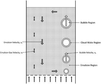 |
| | Fig. 2 Schematic of the bubbling fluidized bed model.46 | |
In this study, we assume the particles are of Geldart group A. Since the process model utilized in this study uses a more complex reaction–diffusion particle model which introduces a second spatial dimension, as described in sections 2–3 above, the original BFB model has been simplified relative to the model described in ref. 46. The gas velocity is well above the minimum fluidization velocity and within the “bubbling fluidization regime”; however, it is assumed that no bubbles are formed. The model utilizes instead a single “emulsion” region/phase where gas is direct contact with the solid particle. The particle length scale is radially discretized (spherical domain) into 30 control volumes. The device length scale is axially discretized (cylindrical domain) into 25 control volumes. Both solid sorbents and flue gas consisting of CO2, H2O, and N2 are injected at the bottom of the bed and flow upward through the absorber as the particles are transported axially through the bed, removing CO2 from the gas.
The model is implemented in Aspen Custom Modeler (ACM) (Aspen Technologies, Inc.). The particle length scale was solved using ACM's partial differential equation (PDE) solver utilizing a 2nd-order central finite difference method. At the process-scale, a compartment-based approach, where axial differential terms were expressed as finite differences involving a first-order forward finite difference method, was used. The physical properties of the gas phase were calculated with the cubic equation of state. The physical properties of the solids were based on experimental measurements. The process model involves 332![[thin space (1/6-em)]](https://www.rsc.org/images/entities/char_2009.gif) 890 equations and a significantly larger number of non-zeroes, as reported by ACM. Computations have been conducted on a Windows-based Workstation utilizing an 8-core Intel i7 Processor.
890 equations and a significantly larger number of non-zeroes, as reported by ACM. Computations have been conducted on a Windows-based Workstation utilizing an 8-core Intel i7 Processor.
The discrepancy terms were evaluated using external procedure calls in ACM. These procedures were coded in C++ and compiled into a dynamic link library for fast evaluation of discrepancy terms and their residuals within the process models. The dynamic discrepancy evaluation framework was automated, with error handling capability, to read each posterior point from an excel spreadsheet and report the corresponding Lagrangian profiles for the solid particles. Due to the large magnitudes of the “step-changes” involved and the presence of external procedure calls, a homotopy-based approach was used.
The process model involves a steady-state evaluation with process conditions varying spatially. However, to analyze the data corresponding to the discrepancy at the particle scale, a conversion to a temporal domain is required. This involves an interpretation of process conditions surrounding individual particles as they axially traverse through the adsorber bed. Hence, a Eulerian to Lagrangian transformation,47 also known as a “material” or “substantive” derivative, is utilized based on the flow velocity of the solid particles in the emulsion region.
Each sample drawn from the posterior distribution involves a simulation of the absorber column within ACM, and the operating conditions and overall CO2 capture in the device are reported.
5 Results
5.1 Posterior distribution
94![[thin space (1/6-em)]](https://www.rsc.org/images/entities/char_2009.gif) 000 MCMC steps were obtained in total. 70
000 MCMC steps were obtained in total. 70![[thin space (1/6-em)]](https://www.rsc.org/images/entities/char_2009.gif) 000 were cut out for burn-in, leaving 24
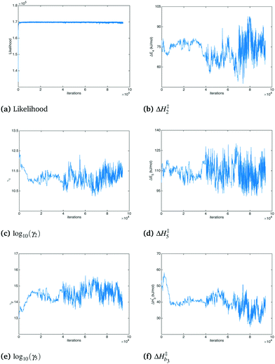
000 were cut out for burn-in, leaving 24![[thin space (1/6-em)]](https://www.rsc.org/images/entities/char_2009.gif) 000 steps in the posterior. Fig. 3 shows the likelihood and a selection of parameters as a function of Monte Carlo step. The movement of the MCMC sampler can be seen in the figure, with a clear equilibration occurring after 70
000 steps in the posterior. Fig. 3 shows the likelihood and a selection of parameters as a function of Monte Carlo step. The movement of the MCMC sampler can be seen in the figure, with a clear equilibration occurring after 70![[thin space (1/6-em)]](https://www.rsc.org/images/entities/char_2009.gif) 000 steps. The posterior samples were separated into approximately 150 batches and t-confidence intervals were produced on the batch means. The analysis reveals that the means of all but a relative handful were estimated to within ±5% with 95% confidence. Some of the parameters whose confidence intervals exceeded ±5% were ΔH2 (±∼6%), ΔH‡2 (±∼7%), ΔS5 (±∼8%), β255 (±∼11%), β1 (±∼14%) and β17 (±∼38%). This final interval is larger than might be desired; however, considering the much tighter intervals for almost every parameter estimated, along with the slow convergence of this single marginal in a distribution with a dimensionality of 279, the convergence of the routine was deemed acceptable.
000 steps. The posterior samples were separated into approximately 150 batches and t-confidence intervals were produced on the batch means. The analysis reveals that the means of all but a relative handful were estimated to within ±5% with 95% confidence. Some of the parameters whose confidence intervals exceeded ±5% were ΔH2 (±∼6%), ΔH‡2 (±∼7%), ΔS5 (±∼8%), β255 (±∼11%), β1 (±∼14%) and β17 (±∼38%). This final interval is larger than might be desired; however, considering the much tighter intervals for almost every parameter estimated, along with the slow convergence of this single marginal in a distribution with a dimensionality of 279, the convergence of the routine was deemed acceptable.
 |
| | Fig. 3 Likelihood and selected model parameters vs. Monte Carlo step. | |
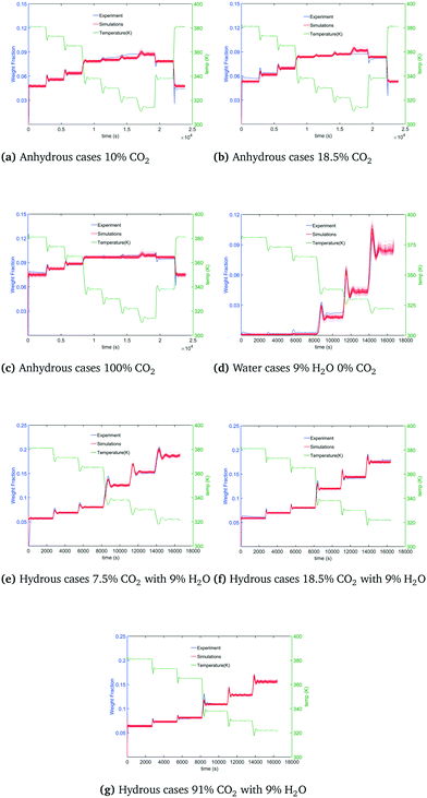
Coverage of the experimental data is shown by reproducing and overlaying a set of model realizations drawn from the posterior against the dynamic TGA data. Fig. 4(b)–(h) shows the coverage of calibration results to the data under dry CO2, H2O and humidified CO2 conditions. The green curve shows the temperature change during the adsorption process. The blue curve is the TGA trace of the weight fraction of adsorbed CO2, and red curves are 100 model realizations drawn from the posterior. TGA data was well covered by calibration results in these seven cases. Relatively small regions of coverage gaps can mostly be attributed to systematic experimental error not considered in the model.
 |
| | Fig. 4 Calibration results under dry and humid conditions. | |
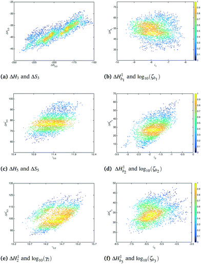
Bivariate scatter plots visualize the correlation between pairs of model parameters. Selected bivariate scatter plots appear in Fig. 5. In the figures, yellow represents regions of high sample density, while blue indicates relatively lower density. Strong correlations appear between certain pairs of model parameters. The correlations between ΔH1 and ΔS1, ΔH3 and ΔS3, and ΔH4 and ΔS4 were 0.98, 0.91 and 0.79, respectively. Generally speaking, the correlation between the formation enthalpy and entropy reflects the functional form of the equilibrium constant. The correlations between  and log10(ςb1),
  and log10(ςb2),
  and log10(ςb3) were 0.98, 0.99 and 0.5, respectively; similarly, these correlations are expected due to the functional form of the mobility.
 |
| | Fig. 5 Bivariate scatter plots of selected model parameters. | |
5.2 Process-scale predictions
Two operational cases were investigated: an adiabatic case (in which the temperature of the bed increases along its length due to the heat of reaction), and a case with external cooling (in which embedded cooling tubes remove excess heat). Within each operational case, dry CO2 inlet and humidified CO2 inlet cases were considered. The dry inlet gas contains 10.9% CO2; the humidified inlet gas contains 10.9% CO2 and 5.5% H2O, balanced in each case withN2. The temperature of the flue gases is 65 °C at the inlet. These compositions are similar to inlet compositions for a post-combustion CO2 adsorber at a coal-fired power plant, operating downstream of SOx and NOx scrubbing systems.
5.2.1 Adiabatic.
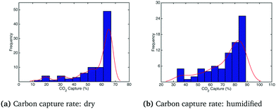
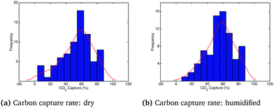
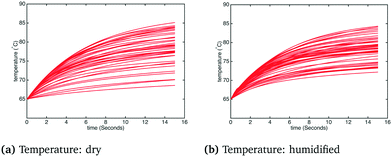
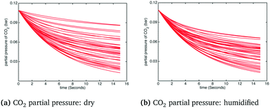
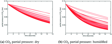
The histogram and kernel smoothing density fit of carbon capture fraction from the dry gas and humidified gas adsorbers in the adiabatic case are shown in Fig. 6. In the dry case – Fig. 6(a) – the mean carbon capture fraction is 0.54 and the 95% credible region for the carbon capture fraction is between 0.14 and 0.94. In the humidified case – Fig. 6(b) – the mean carbon capture fraction is 0.56 and the 95% credible region is between 0.24 and 0.88. In both cases the significant uncertainty in the capture rate reflects the paucity of kinetic data appearing in the dynamic TGA used for calibration. The small difference in the mean capture rate reflects the fact that water is barely adsorbed when the temperature is higher than 75 °C, which is quickly exceeded in the adiabatic case (reaching in some cases temperatures as high as 85 °C) as particles move through the bed. Forty realizations from the posterior showing the operating temperature and CO2 partial pressure in the bed for the adiabatic case are shown in Fig. 7 and 8, respectively.§
 |
| | Fig. 6 Carbon capture rate under dry and humidified CO2 conditions for the adiabatic case. | |
 |
| | Fig. 7 Temperature in the adsorber under dry and humidified CO2 conditions for the adiabatic case. | |
 |
| | Fig. 8 CO2 partial pressure in the adsorber under dry and humidified CO2 conditions for the adiabatic case. | |
5.2.2 External cooling.
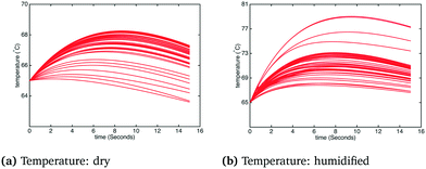
In order to observe a larger influence of water on the process, external cooling (water at 20 °C, 209 kg s−1) was added to internal heat transfer tubes within the BFB model. The corresponding influence on the adsorber operating temperature is shown in Fig. 9: the significant suppression of the reactor temperature means that more water from the flue gas will adsorb on the sorbent, with attendant increase of the effective CO2 capacity according to the kinetic model. In this case the differences in the temperature profiles between dry and humidified cases are much more pronounced. These differences are also reflected in the CO2 capture fraction distributions with external cooling, as shown in Fig. 10. In the dry case – Fig. 10(a) – the mean carbon capture fraction is 0.56 (only slightly higher than the case without cooling) and the 95% credible region for the carbon capture fraction is 0.28 and 0.84. In the humidified case – Fig. 10(b) – the mean carbon capture fraction is 0.73 and the 95% credible region is between 0.47 and 0.99, reflecting a considerable increase over the case without cooling. The CO2 partial pressure profiles in the adsorber for both dry and humidified cases are shown in Fig. 11.
 |
| | Fig. 9 Temperature under dry and humidified CO2 conditions with external cooling. | |
 |
| | Fig. 10 Distributions of carbon capture rate under dry and humidified CO2 conditions with external cooling. | |
 |
| | Fig. 11 CO2 partial pressure under humidified CO2 conditions with external cooling. | |
6 Discussion
The results of the study demonstrate both the feasibility and the value of the DDRM method for incorporating sophisticated chemical models into process-scale simulations. The benefits of using such a detailed kinetic model at the process-scale is apparent in the external cooling cases, for which significant differences in the capture rates between the dry and humidified cases were revealed, reflecting the influence of water on CO2 diffusion and adsorption embodied in the chemical model. Simpler kinetic models such as the model appearing in ref. 17 lack the relationship between H2O and the diffusivity of CO2 in the sorbent.
The stochastic nature of the predictions is another key advantage of the DDRM method and the associated uncertainty-based paradigm for multi-scale modeling. The process-scale simulations force extrapolation in the kinetic model, as revealed by the relatively large uncertainty in the process results compared to the tightness of the fits to the dynamic TGA data. The uncertainty in the results can provide a more reliable basis for process design and scale up, in particular when combined with strategies for optimization under uncertainty.
Physically speaking, discrepancy functions represent interactions among chemical species in a model which, without discrepancy, ignores such interactions. In principle, the discrepancy functions should thus depend on all chemical states in the system plus the temperature: for the equilibrium constants, it would suffice to make the discrepancy functions depend on all partial pressures in the system; for the transport coefficients, all of the chemical species within the solid. Such an approach would be comprehensive; however, it would also increase the number of terms for calibration. As such this study limited the dependency of each discrepancy function to a single chemical constituent plus the temperature, which proved to be sufficient for this study. Future work will explore methods for generalizing the dependence of the discrepancy functions while limiting the number of variables for calibration.
In this work, the discrepancy enables fully quantitative correspondence between the model and the data. The physical model provides a semi-quantitative correspondence to the same dataset, as seen in ref. 16. The stochastic functions thus provide the increase in variability required for fully quantitative correspondence between model and experiment (as seen in this paper), along with model reduction that enables calibration and propagation of uncertainty.
In the present study, the predictions at the process-scale reflect a significant amount of uncertainty in the kinetics. This can be attributed to the relative dearth of kinetic information in the dynamic TGA experiment, thus motivating alternative bench-scale experiments (such as fixed bed) that may yield more useful data. The stochastic process-scale results present opportunities for the design of such experiments due to the dynamic results for bed temperature and gas composition: each curve depicted in Fig. 9 and 11, for instance, represents a dynamically changing set of conditions that bench-scale experiments could attempt to replicate. Adding a sampling of conditions drawn from these figures to the set of experiments used for model calibration would very likely decrease the uncertainty in the process-scale predictions. Integration of the method with bench-scale experimentation, flowsheet modeling and optimization under uncertainty presents significant opportunities for decreasing the time and costs of scale-up through more accurate modeling of industrial scale systems.
7 Conclusions
“Dynamic discrepancy reduced modeling” is a method of order reduction introduced in this work in which states of a large dynamic system are removed and the error thereby introduced is corrected with Gaussian process stochastic functions applied intrusively within the kinetic model. The result is a stochastic model which robustly and efficiently quantifies and propagates uncertainty in the kinetic model to the process scale. DDRM is a critical component of an uncertainty-based methodology for bench-to-process scale-bridging. The method is made possible through the nature of the BSS-ANOVA GPs, which in Karhunen–Loéve-expanded form constrain stochasticity to the coefficients of the expansion, thus enabling the solution of deterministic models in the core MCMC sampling process. In this first significant demonstration of the power of the DDRM method, the order of a reaction–diffusion model for the adsorption process in mesoporous silica-supported amine-impregnated sorbents was reduced by decreasing the resolution of the diffusion model, and BSS-ANOVA GPs were incorporated into the diffusion coefficients. The process-scale results confirm the importance of the detailed treatment of the adsorption reaction for highly loaded amine sorbents.
Acknowledgements
Funding for this work was provided by the Department of Energy through the Carbon Capture Simulation Initiative. This report was prepared as an account of work sponsored by an agency of the United States Government. Neither the United States Government nor any agency thereof, nor any of their employees, makes any warranty, express or implied, or assumes any legal liability or responsibility for the accuracy, completeness, or usefulness of any information, apparatus, product, or process disclosed, or represents that its use would not infringe privately owned rights. Reference herein to any specific commercial product, process, or service by trade name, trademark, manufacturer, or otherwise does not necessarily constitute or imply its endorsement, recommendation, or favoring by the United States Government or any agency thereof. The views and opinions of authors expressed herein do not necessarily state or reflect those of the United States Government or any agency thereof.
References
-
J. T. Houghton, Climate change 1995: The science of climate change: contribution of working group I to the second assessment report of the Intergovernmental Panel on Climate Change, Cambridge University Press, 1996 Search PubMed.
-
J. H. Butler and S. Montzka, The NOAA annual greenhouse gas index, Noaa earth system research laboratory technical report, 2011 Search PubMed.
- M. K. Mondal, H. K. Balsora and P. Varshney, Energy, 2012, 46, 431–441 CrossRef CAS.
- A. B. Rao and E. S. Rubin, Environ. Sci. Technol., 2002, 36, 4467–4475 CrossRef CAS PubMed.
- J. Davison, Energy, 2007, 32, 1163–1176 CrossRef CAS.
- A. Samanta, A. Zhao, G. K. Shimizu, P. Sarkar and R. Gupta, Ind. Eng. Chem. Res., 2011, 51, 1438–1463 CrossRef.
- A. S. Bhown and B. C. Freeman, Environ. Sci. Technol., 2011, 45, 8624–8632 CrossRef CAS PubMed.
- M. Wang, A. Lawal, P. Stephenson, J. Sidders and C. Ramshaw, Chem. Eng. Res. Des., 2011, 89, 1609–1624 CrossRef CAS.
- D. C. Miller, J. T. Litynski, L. A. Brickett and B. D. Morreale, AIChE J., 2016, 62, 2–10 CrossRef CAS.
- D. C. Miller, M. Syamlal, D. S. Mebane, C. Storlie, D. Bhattacharyya, N. V. Sahinidis, D. Agarwal, C. Tong, S. E. Zitney, A. Sarkar, X. Sun, S. Sundaresan, E. Ryan, D. Engel and C. Dale, Annu. Rev. Chem. Biomol. Eng., 2014, 5, 301–323 CrossRef CAS PubMed.
-
H. Simon, T. Zacharia and R. Stevens, et al., Modeling and Simulation at the Exascale for Energy and the Environment, Department of Energy Technical Report, 2007 Search PubMed.
- X. Jiang, Appl. Energy, 2011, 88, 3557–3566 CrossRef CAS.
-
D. C. Miller, D. A. Agarwal, X. Sun and C. Tong, “CCSI and the role of advanced computing in accelerating the commercial deployment of carbon capture systems,” Proceedings of the SciDAC 2011 Conference, 2011 Search PubMed.
-
D. C. Miller, M. Syamlal, J. Meza, D. Brown, M. Fox, M. Khaleel, R. Cottrell, J. Kress, X. Sun and S. Sundaresan, et al., “Overview of the US DOE's Carbon Capture Simulation Initiative for accelerating the commercialization of CCS technology,” 36th International Technical Conference on Clean Coal & Fuel Systems, 2011 Search PubMed.
- D. S. Mebane, J. D. Kress, C. B. Storlie, D. J. Fauth, M. L. Gray and K. Li, J. Phys. Chem. C, 2013, 117, 26617–26627 CAS.
- K. Li, J. D. Kress and D. S. Mebane, J. Phys. Chem. C, 2016, 120, 23683–23691 CAS.
-
A. Lee, D. Mebane, D. Fauth and D. Miller, “A model for the adsorption kinetics of CO2 on amine-impregnated mesoporous sorbents in the presence of water,” 28th International Pittsburgh Coal Conference, Pittsburgh, PA, 2011 Search PubMed.
- K. S. Bhat, D. S. Mebane, C. B. Storlie and P. Mahapatra, J. Am. Stat. Assoc., 2017 DOI:10.1080/01621459.2017.1295863 , in press.
- B. Reich, C. Storlie and H. Bondell, Technometrics, 2009, 51, 110–120 CrossRef PubMed.
- M. C. Kennedy and A. O'Hagan, J. R. Stat. Soc. Ser. B Stat. Methodol., 2001, 63, 425–464 Search PubMed.
- M. Van Oijen, J. Rougier and R. Smith, Tree Physiol., 2005, 25, 915–927 CrossRef PubMed.
- M. Van Oijen, C. Reyer, F. Bohn, D. Cameron, G. Deckmyn, M. Flechsig, S. Härkönen, F. Hartig, A. Huth and A. Kiviste,
et al.
, For. Ecol. Manage., 2013, 289, 255–268 CrossRef.
- D. Higdon, C. Nakhleh, J. Gattiker and B. Williams, Comput. Methods Appl. Mech. Eng., 2008, 197, 2431–2441 CrossRef.
- F. Liu, M. Bayarri, J. Berger, R. Paulo and J. Sacks, Comput. Methods Appl. Mech. Eng., 2008, 197, 2457–2466 CrossRef.
- G. B. Arhonditsis, D. Papantou, W. Zhang, G. Perhar, E. Massos and M. Shi, J. Mar. Syst., 2008, 73, 8–30 CrossRef.
- A. Van Griensven and T. Meixner, J. Hydroinf., 2007, 9, 277–291 CrossRef.
- W. Zhang and G. B. Arhonditsis, J. Great Lakes Res., 2008, 34, 698–720 CrossRef CAS.
- D. Kavetski, G. Kuczera and S. W. Franks, Water Resour. Res., 2006, 42, W03408 Search PubMed.
- E. Jeremiah, S. Sisson, L. Marshall, R. Mehrotra and A. Sharma, Water Resour. Res., 2011, 47, W07547 CrossRef.
- P. M. Tagade, B.-M. Jeong and H.-L. Choi, Build. Environ., 2013, 70, 232–244 CrossRef.
-
J.-X. Wang, C. J. Roy and H. Xiao, 2015, arXiv preprint arXiv:1501.03189.
- D. S. Mebane, K. S. Bhat, J. D. Kress, D. J. Fauth, M. L. Gray, A. Lee and D. C. Miller, Phys. Chem. Chem. Phys., 2013, 15, 4355–4366 RSC.
- J. C. Eslick, B. Ng, Q. Gao, C. H. Tong, N. V. Sahinidis and D. C. Miller, Energy Procedia, 2014, 63, 1055–1063 CrossRef CAS.
- B. Konomi, G. Karagiannis, A. Sarkar, X. Sun and G. Lin, Technometrics, 2014, 56, 145–158 CrossRef.
- C. Lai, Z. Xu, W. Pan, X. Sun, C. Storlie, P. Marcy, J.-F. Dietiker, T. Li and J. Spenik, Powder Technol., 2016, 288, 388–406 CrossRef CAS.
- J. Kalyanaraman, Y. Kawajiri, R. P. Lively and M. J. Realff, AIChE J., 2016, 62, 3352–3368 CrossRef CAS.
- J. Kalyanaraman, Y. F. Fan, Y. Labreche, R. P. Lively, Y. Kawajiri and M. J. Realff, Comput. Chem. Eng., 2015, 81, 376–388 CrossRef CAS.
- C. B. Storlie, M. L. Fugate, D. M. Higdon, A. V. Huzurbazar, E. G. Francois and D. C. McHugh, Technometrics, 2013, 55, 436–449 CrossRef.
-
A. Berlinet and C. Thomas-Agnan, Reproducing kernel Hilbert spaces in probability and statistics, Kluwer Academic Boston, 2004, vol. 3 Search PubMed.
-
A. Berlinet and C. Thomas-Agnan, Reproducing kernel Hilbert spaces in probability and statistics, Springer Science & Business Media, 2011 Search PubMed.
- C. B. Storlie, W. A. Lane, E. M. Ryan, J. R. Gattiker and D. M. Higdon, J. Am. Stat. Assoc., 2015, 110, 68–82 CrossRef CAS.
- W. K. Hastings, Biometrika, 1970, 57, 97–109 CrossRef.
-
W. R. Gilks, S. Richardson and D. J. Spiegelhalter, Markov Chain Monte Carlo in practice, Chapman & Hall/CRC, 1996 Search PubMed.
- S. Geman and D. Geman, IEEE Trans. Pattern Anal. Mach. Intell., 1984, 721–741 CrossRef CAS.
- H. Haario, E. Saksman and J. Tamminen, Bernoulli, 2001, 223–242 CrossRef.
- A. Lee and D. C. Miller, Ind. Eng. Chem. Res., 2012, 52, 469–484 Search PubMed.
-
R. Bird, W. Stewart and E. Lightfoot, Transport Phenomena (revised second ed.), John Wiley & Sons, 2007 Search PubMed.
Footnotes |
| † The Los Alamos National Laboratory is operated by Los Alamos National Security, LLC for the National Nuclear Security Administration of the U.S. Department of Energy under Contract No. DE-AC52-06NA25396. |
| ‡ The functions defined in this section pertain to thermodynamic quantities and thus need not be strictly dynamic; in the particular calibration case treated here they are still dynamic because T changes with time. |
| § In all figures depicting the conditions inside the bed, time on the x-axis denotes residence time for a population-averaged particle moving through the bed. It is thus proportional to bed depth. |
|
| This journal is © The Royal Society of Chemistry 2017 |
Click here to see how this site uses Cookies. View our privacy policy here.  d and
David S.
Mebane
 *a
*a


![[scr P, script letter P]](https://www.rsc.org/images/entities/char_e52f.gif) (θ∣Z) is the posterior: the probability of θ given dataset Z;
(θ∣Z) is the posterior: the probability of θ given dataset Z; ![[scr P, script letter P]](https://www.rsc.org/images/entities/char_e52f.gif) (Z∣θ) is the likelihood: the probability of observing the data given θ, which must include a model for the observation error; and
(Z∣θ) is the likelihood: the probability of observing the data given θ, which must include a model for the observation error; and ![[scr P, script letter P]](https://www.rsc.org/images/entities/char_e52f.gif) (θ) is the prior. The integral in the denominator is the probability of observing the particular dataset Z (Z is considered to be an observation of a stochastic variable
(θ) is the prior. The integral in the denominator is the probability of observing the particular dataset Z (Z is considered to be an observation of a stochastic variable  ) over all possible values of θ, called marginal likelihood or marginal density of the observations.


![[scr O, script letter O]](https://www.rsc.org/images/entities/char_e52e.gif) (N3) for a traditional GP.18,38
(N3) for a traditional GP.18,38


![[small theta, Greek, macron]](https://www.rsc.org/images/entities/i_char_e0c9.gif) = [
= [![[small theta, Greek, macron]](https://www.rsc.org/images/entities/i_char_e0c9.gif) 1,...,
1,...,![[small theta, Greek, macron]](https://www.rsc.org/images/entities/i_char_e0c9.gif) 23] fixed at the current point in the random walk, and covariance matrix V is the empirical covariance of a subset of the previously accepted values in the MCMC chain:
23] fixed at the current point in the random walk, and covariance matrix V is the empirical covariance of a subset of the previously accepted values in the MCMC chain:

![[thin space (1/6-em)]](https://www.rsc.org/images/entities/char_2009.gif) 890 equations and a significantly larger number of non-zeroes, as reported by ACM. Computations have been conducted on a Windows-based Workstation utilizing an 8-core Intel i7 Processor.
890 equations and a significantly larger number of non-zeroes, as reported by ACM. Computations have been conducted on a Windows-based Workstation utilizing an 8-core Intel i7 Processor.![[thin space (1/6-em)]](https://www.rsc.org/images/entities/char_2009.gif) 000 MCMC steps were obtained in total. 70
000 MCMC steps were obtained in total. 70![[thin space (1/6-em)]](https://www.rsc.org/images/entities/char_2009.gif) 000 were cut out for burn-in, leaving 24
000 were cut out for burn-in, leaving 24![[thin space (1/6-em)]](https://www.rsc.org/images/entities/char_2009.gif) 000 steps in the posterior. Fig. 3 shows the likelihood and a selection of parameters as a function of Monte Carlo step. The movement of the MCMC sampler can be seen in the figure, with a clear equilibration occurring after 70
000 steps in the posterior. Fig. 3 shows the likelihood and a selection of parameters as a function of Monte Carlo step. The movement of the MCMC sampler can be seen in the figure, with a clear equilibration occurring after 70![[thin space (1/6-em)]](https://www.rsc.org/images/entities/char_2009.gif) 000 steps. The posterior samples were separated into approximately 150 batches and t-confidence intervals were produced on the batch means. The analysis reveals that the means of all but a relative handful were estimated to within ±5% with 95% confidence. Some of the parameters whose confidence intervals exceeded ±5% were ΔH2 (±∼6%), ΔH‡2 (±∼7%), ΔS5 (±∼8%), β255 (±∼11%), β1 (±∼14%) and β17 (±∼38%). This final interval is larger than might be desired; however, considering the much tighter intervals for almost every parameter estimated, along with the slow convergence of this single marginal in a distribution with a dimensionality of 279, the convergence of the routine was deemed acceptable.
000 steps. The posterior samples were separated into approximately 150 batches and t-confidence intervals were produced on the batch means. The analysis reveals that the means of all but a relative handful were estimated to within ±5% with 95% confidence. Some of the parameters whose confidence intervals exceeded ±5% were ΔH2 (±∼6%), ΔH‡2 (±∼7%), ΔS5 (±∼8%), β255 (±∼11%), β1 (±∼14%) and β17 (±∼38%). This final interval is larger than might be desired; however, considering the much tighter intervals for almost every parameter estimated, along with the slow convergence of this single marginal in a distribution with a dimensionality of 279, the convergence of the routine was deemed acceptable.
 and log10(ςb1),
  and log10(ςb2),
  and log10(ςb3) were 0.98, 0.99 and 0.5, respectively; similarly, these correlations are expected due to the functional form of the mobility.